PROPERTIES OF THE TRANS-NEPTUNIAN BELT: STATISTICS FROM THE CFHT SURVEY

Abstract

We present the results of a wide-field survey designed to measure the size, inclination, and radial distributions of Kuiper Belt Objects (KBOs). The survey found 86 KBOs in 73 square degrees observed to limiting red magnitude 23.7 using the Canada-France-Hawaii Telescope and the 12k x 8k CCD Mosaic camera. For the first time, both ecliptic and off-ecliptic fields were examined to more accurately constrain the inclination distribution of the KBOs. The survey data were processed using an automatic moving object detection algorithm, allowing a careful characterization of the biases involved. In this work, we quantify fundamental parameters of the Classical KBOs (CKBOs), the most numerous objects found in our sample, using the new data and a maximum likelihood simulation. Deriving results from our best-fit model, we find that the size distribution follows a differential power law with exponent $q=4.0^{+0.6}_{-0.5}$ ($1\sigma$, or 68.27% confidence). In addition, the CKBOs inhabit a very thick disk consistent with a Gaussian distribution of inclinations with a Half-Width of $i_{1/2}=20\arcdeg^{+6\arcdeg}_{-4\arcdeg}$ (1 $\sigma$). We estimate that there are $N_{\rm CKBOs}(D>100\mbox{ km})=3.8^{+2.0}_{-1.5}\times 10^{4}$ ($1\sigma$) CKBOs larger than 100 km in diameter. We also find compelling evidence for an outer edge to the CKBOs at heliocentric distance $R=50$ AU.

1 Introduction

The rate of discovery of Kuiper Belt Objects (KBOs) has increased dramatically since the first member (1992 $\rm QB_{1}$) was found (Jewitt & Luu 1993). As of Dec 2000, $\sim 400$ KBOs are known. These bodies exist in three dynamical classes (Jewitt, Luu & Trujillo 1998): (1) the Classical KBOs (CKBOs) occupy nearly circular (eccentricities $e<0.25$) orbits with semimajor axes $41\mbox{ AU}\lesssim a\lesssim 46\mbox{ AU}$, and they constitute $\sim 70$ % of the observed population; (2) the Resonant KBOs occupy mean-motion resonances with Neptune, such as the 3:2 (the Plutinos, $a\approx 39.4$ AU) and 2:1 ($a\approx 47.8$ AU), and comprise $\sim 20$ % of the known objects; (3) the Scattered KBOs represent only $\sim 10$ % of the known KBOs, but possess the most extreme orbits, with median semimajor axis $a\sim 90$ AU and eccentricity $e\sim 0.6$, presumably due to a weak interaction with Neptune (Duncan & Levison 1997, Luu et al. 1997, and Trujillo, Jewitt & Luu 2000). Although these classes are now well established, only rudimentary information has been collected about their populations. One reason is that only a fraction of the known KBOs were discovered in well-parametrized surveys that have been published in the open literature (principally Jewitt & Luu 1993 (1 KBO); Jewitt & Luu 1995 (17 KBOs); Irwin, Tremaine & Żytkow 1995 (2 KBOs); Jewitt, Luu & Chen 1996 (15 KBOs); Gladman et al. 1998 (5 KBOs); Jewitt, Luu & Trujillo 1998 (13 KBOs); and Chiang & Brown 1999 (2 KBOs)). In this work, we characterize the fundamental parameters of the CKBOs: the size distribution, inclination distribution and radial distribution using a large sample (86 KBOs) discovered in a well-characterized survey.

The quintessential measurement of the size distribution relies on the Cumulative Luminosity Function (CLF). The CLF describes the number of KBOs $\mbox{deg}^{-2}$ ($\Sigma$) near the ecliptic as a function of apparent red magnitude ($m_{R}$). It is fitted with the relation $\log(\Sigma)=\alpha(m_{R}-m_{0})$, where $m_{0}$ is the red magnitude at which $\Sigma=1$ KBO $\mbox{deg}^{-2}$. The slope ($\alpha$) is related to the size distribution (described later). Although many different works have considered the CLF, two papers are responsible for discovering the majority of KBOs found in published surveys: Jewitt, Luu & Chen (1996) and Jewitt, Luu & Trujillo (1998). The former constrained the CLF over a 1.6 magnitude range ($23.2<m_{R}<24.8$) with 15 discovered KBOs while the latter covered a complimentary 2.5 magnitude range ($20.5<m_{R}<23.0$), discovering 13 objects. Jewitt, Luu & Trujillo (1998) measured the CLF produced from these two data sets and found $\alpha=0.58\pm 0.05$ and $m_{0}=23.27\pm 0.11$. Gladman et al. (1998) criticized this work on 2 main counts: (1) they believed that Jewitt, Luu & Chen (1996) underestimated the number of KBOs and (2) the fit in the Jewitt, Luu & Trujillo (1998) survey used a least-squares approach that assumed Gaussian errors rather than Poissonian errors. Gladman et al. (1998) found 5 additional KBOs and re-analysed the CLF using a Poissonian maximum likelihood method to refit the CLF to (1) the Jewitt, Luu & Trujillo (1998) data without the Jewitt, Luu & Chen (1996) data and (2) a fit to the 6 different surveys available at the time except for Tombaugh (1961), Kowal (1989) and Jewitt, Luu & Chen (1996). Both of these fits were steeper but formally consistent with the original Jewitt, Luu & Trujillo (1998) data at the $\sim 1.5\sigma$ level: (1) $\alpha=0.72^{+0.30}_{-0.26}$ and $m_{0}=23.3^{+0.2}_{-0.4}$ and (2) $\alpha=0.76^{+0.10}_{-0.11}$ and $m_{0}=23.40^{+0.20}_{-0.18}$. Chiang & Brown (1999) find a flatter size distribution of $\alpha=0.52\pm 0.05$ and $m_{0}=23.5\pm 0.06$ much closer to the Jewitt, Luu & Trujillo (1998) result. They observed that the steep size distribution reported by Gladman et al. (1998) was an artifact of their selective exclusion of part of the available survey data, not of their use of a different fitting method. The first goal of this work is to measure the CLF and additionally constrain the power-law slope of the size distribution using a single well-characterized survey and a maximum likelihood simulation which allows for the correction of observational biases.

An accurate characterization of the inclination distribution of the KBOs is critical to understanding the dynamical history of the outer Solar System since the era of planetesimal formation. We expect that the KBOs formed by accretion in a very thin disk of particles with a small internal velocity dispersion (e.g. Kenyon & Luu 1998 and Hahn & Malhotra 1999) and a correspondingly small inclination distribution. However, the velocity dispersion indicated by the inclination distribution in the present-day Kuiper Belt is large. Jewitt, Luu & Chen (1996) measured the apparent Half-Width of the Kuiper Belt inclination distribution to be $\sim 5^{\circ}$. They noted a strong bias against observing high inclination objects in ecliptic surveys, and they estimated the true distribution to be much thicker, with an inclination distribution Half-Width of $\gtrsim 15^{\circ}$, corresponding to a vertical velocity dispersion of $\sim 1$ km/s. Several conjectures have been advanced to explain the thickness of the Kuiper Belt: Earth-mass planetesimals may have been scattered through the belt in the late stages of the planet-formation era, exciting the Kuiper Belt (Morbidelli & Valsecchi 1997 and Petit et al. 1999); stellar encounters may have enhanced the velocity dispersion of the distant KBOs (Ida, Larwood & Burkert, 2000); and the dispersion velocity of small bodies tends to grow to roughly equal the escape speed of the bodies contributing the most mass (the large bodies for size distributions with $q<4$) in the belt (Aarseth, Lin & Palmer 1993). As there is much speculation about the origin of the large velocity dispersion of the Kuiper Belt, but only one published measurement (Jewitt, Luu & Chen 1996), the second goal of this work is to accurately quantify the inclination distribution from our large sample of objects.

The radial extent of the Classical Kuiper Belt has not been well constrained. None of the CKBOs have been discovered beyond $R\approx 50$ AU. This trend was first noted by Dones (1997) who suggested that the 50–75 AU region may be depleted; he found the results of a Monte-Carlo simulation of CKBOs drawn from a rather flat differential size distribution (power-law index $q=3$) to be inconsistent with the observations of the 6 CKBOs discovered by Jewitt, Luu & Chen (1996). Jewitt, Luu & Trujillo (1998) discovered all of their KBOs at heliocentric distances $R<46$ AU. In the absence of other effects, one should expect to find fewer bodies with $R>50$ AU than with $R\sim 40$ AU, as the former are about a magnitude fainter than the latter. However, through the use of a Monte-Carlo model they demonstrated that the bias against objects beyond 50 AU is not strong enough to explain the distribution of discovery distances. They speculated that the lack of bodies discovered beyond 50 AU could be caused by a combination of (1) a decrease in the maximum KBO size (and reduction in the brightest and most detectable objects) beyond 50 AU or (2) the size distribution might steepen beyond 50 AU, putting more of the mass in the smaller, less-detectable bodies. They also suggested that the lack of $R>50$ AU objects could be explained by an outer edge to the Classical Kuiper Belt at 50 AU.

Two later papers questioned the existence of an edge to the Kuiper Belt near 50 AU. Gladman et al. (1998) suggested that the number of objects expected to be discovered beyond 50 AU is highly dependent on the size distribution because steep size distributions reduce the number of large (bright) bodies relative to small (faint) bodies. Gladman et al. (1998) adopted a relatively steep distribution ($q=4.65$), and found no significant evidence of a truncated belt. Chiang & Brown (1999) found that 8%–13% of the $\sim 100$ objects known at the time should have been found beyond 50 AU, and suggested that this precludes the presence of a density enhancement beyond 50 AU, but could not definitively rule out a density deficit. Allen, Bernstein & Malhotra (2001) have also recently reported the detection of an outer edge to the Kuiper Belt. The third goal of the present work is to test the distribution of the discovery distances for the presence of an outer edge to the Kuiper Belt.

2 Survey Data

Observations were made at the 3.6 m diameter Canada-France-Hawaii Telescope using the 12288 x 8192, 15 µm pixel mosaic CCD (CFHT 12k; Cuillandre et al. 2000). Built at the University of Hawaii (UH) the CFHT 12k comprises 12 edge-abutted, thinned, high quantum efficiency (QE $\sim 0.75$), 4096 x 2048 pixel Lincoln Laboratory CCDs. It is currently the largest close-packed CCD camera in the world. When mounted at the CFHT f/4 prime focus the camera yields a plate scale of 0.206 arc sec/pixel, corresponding to a 0.330 sq deg field of view in each 200 Mbyte image. Images were taken through a Mould $R$ filter, with a central wavelength of 6581 Å and a bandwidth of 1251 Å. Instrumental parameters of the survey are summarized in Table 1.

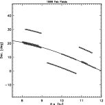
Figure 1: Fields imaged in Feb 1999. The ecliptic is denoted by a solid line.

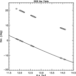
Figure 3: Fields imaged in Mar 2000. The ecliptic is denoted by a solid line.

Observations were taken within a few days of new moon under photometric conditions during three periods: Feb 10 – 15 1999, Sep 5–8 1999, and Mar 31 – Apr 3 2000. Fields were imaged at airmasses $<1.7$ and were within 1.5 hours of opposition. We chose to use short 180 s exposures at the CFHT to maximize area coverage and detection statistics. All discovered objects were accessible for recovery at the UH 2.2 m telescope during comparable seeing conditions with exposure times of $<600$ seconds. Each field was imaged three times (a “field triplet”), with about 1 hour timebase between exposures. Fields imaged appear in Figures 1, 2 and 3, and in Table 3. The CFHT observations were taken at three ecliptic latitudes $\beta=0^{\circ}$, $10^{\circ}$, and $20^{\circ}$ to probe the inclination distribution of the KBOs (see §4).

Photometric calibrations were obtained from Landolt (1992) standard stars imaged several times on each chip. Three CFHT 12k chips of poor quality were replaced between the Feb 1999 and Sep 1999 runs. The positions of four other CFHT 12k chips within the focal plane array were changed to move the cosmetically superior chips towards the center of the camera. The photometric calibration accounts for these changes, as shown in Table 2, containing the measured photometric zero points of the chips. In addition, chip 6 was not used in Feb 1999 because of its extremely poor cosmetic quality. The area covered in the fields from Feb 1999 was corrected for this 8% reduction in field-of-view. The area imaged in Mar 2000 included some small field overlap (6%), resulting in a minor correction applied to the reported total area surveyed.

Each of the 12 CCDs in the CFHT 12k functions as an individual detector, with its own characteristic bias level, flat field, gain level, and orientation (at the $\sim 1^{\circ}$ level). The bias level for each chip was estimated using the row-by-row median of the overscan region. Flat fields were constructed from a combination of (1) the median of normalized bias-subtracted twilight flat fields and (2) a median of bias-subtracted data frames, with a clipping algorithm used to remove excess counts due to bright stars. Fields were analysed by subtracting the overscan region, dividing by the composite flats and searching for moving objects using our Moving Object Detection Software (MODS, Trujillo & Jewitt 1998). We rejected bad pixels through the use of a bad pixel mask.

Artificial moving objects were added to the data to quantify the sensitivity of the moving object detection procedure (Trujillo & Jewitt 1998). The seeing during the survey typically varied from 0.7 arc sec to 1.1 arc sec (FWHM). Accordingly, we subdivided and analysed the data in 3 groups based on the seeing. Artificial moving objects were added to bias-subtracted twilight sky-flattened images, with profiles matched to the characteristic point-spread function for each image group. These images were then passed through the data analysis pipeline. The detection efficiency was found to be uniform with respect to sky-plane speed in the 1 – 10 arc sec/hr range. At opposition, the apparent speed in arc sec/hr, $\dot{\theta}$, of an object is dominated by the parallactic motion of the Earth, and follows

$$\dot{\theta}\approx 148\left(\frac{1-R^{-0.5}}{R-1}\right),$$ (1)

where $R$ is heliocentric distance in AU (Luu & Jewitt 1988). From Equation 1, our speed limit criterion for the survey, $1\mbox{ \arcsec}\mbox{ hr}^{-1}<\dot{\theta}<10\mbox{ \arcsec}\mbox{ hr}^{-1}$, corresponds to opposition heliocentric distances $10\mbox{ AU}\lesssim R\lesssim 140\mbox{ AU}$, with efficiency variations within this range due only to object brightness and seeing.

The magnitude-dependent efficiency function was fitted by

$$\varepsilon=\frac{\varepsilon_{\rm max}}{2}\left(\tanh\left(\frac{m_{R50}-m_{R}}{\sigma}\right)+1\right),$$ (2)

where $0<\varepsilon<1$ is the efficiency with which objects of red magnitude $m_{R}$ are detected, $\varepsilon_{\rm max}$ is the maximum efficiency, $m_{R50}$ is the magnitude at which $\varepsilon=\varepsilon_{\rm max}/2$, and $\sigma$ magnitudes is the characteristic range over which the efficiency drops from $\varepsilon_{\rm max}$ to zero. Table 4 shows the efficiency function derived for each seeing category, along with an average of the seeing cases, weighted by sky area imaged, applicable to the entire data set. The efficiency function is known to greater precision than the $\sim 0.1$ magnitude uncertainty on our discovery photometry. Changes to the efficiency function of $<0.1$ magnitudes produce no significant variation in our results for the size or inclination distributions.

The MODS software, running on two Ultra 10 computers, was fast enough to efficiently search for the KBOs in near real-time, so that newly detected objects could be quickly discovered and re-imaged. We imaged $\sim 35$ field triplets each night at the CFHT, corresponding to $\sim 20$ Gbytes of raw data collected per night, plus several more Gbytes for flat fields and standard stars. Eighty-six KBOs were found in the CFHT survey, 2 of which were serendipitous re-detections of known objects. The discovery conditions of the detected objects appear in Table 5. Photometry was performed using a 2.5 arc second diameter synthetic aperture for discovery data, resulting in median photometric error of 0.15 magnitudes and a maximum photometric error of 0.3 for the faintest objects. Our results are unaffected by this error; randomly introducing $\pm 0.15$ magnitude errors in our simulations (described later), and $\pm 0.3$ magnitude errors in the faintest objects produced no statistically significant change. Trailing loss was insignificant as the KBOs moved only 0.15 arc sec during our integration.

2.1 Recovery Observations and Orbits

Extensive efforts were made to recover all objects using the UH 2.2 m telescope. Attempts were made to recover the objects one week after discovery, then one, two and three months after discovery. Most of these attempts were successful, as demonstrated by the fact that 79 of the 86 CFHT objects were recovered. The loss of 7 objects is the result of unusually poor weather during the Mar–May 1999 recovery period. Only 6 of the 79 recovered objects have arc-lengths shorter than 30 days as of Dec 1, 2000. Second opposition observations have been acquired for 36 of the 78 KBOs found in Feb 1999 and Sep 1999.

Orbits derived from the discovery and recovery data appear in Table 6. The listed elements are those computed by Brian Marsden of the Minor Planet Center. We also benefited from orbital element calculations by David Tholen (Univ. of Hawaii). Both sources produced comparable orbital solutions to the astrometric data.

With only first opposition observations, the inclination and heliocentric distance at discovery can be well determined for nearly all KBOs, as depicted in Figure 4. We find that the semimajor axis and eccentricity determinations are less reliable but are usually good enough to classify the objects as either Classical, Resonance or Scattered KBOs, as depicted in Figure 5. We find that 6 out of 36 (17%) of the objects exhibit orbital changes large enough for their dynamical classification to change from the first opposition to the second opposition. Randomly rejecting 17% of our sample (to simulate misclassification) does not significantly change the results. In addition, rejection of all but the multi-opposition objects does not significantly change our results; as expected, the total number of KBOs estimated decreased by a factor $\sim 2$ and error bars increased by a factor $\sim\sqrt{2}$ due to the sample size reduction. The eccentricity and semimajor axes of all objects with $a<50$ AU (this includes all Classical KBOs) appear in Figure 6.

In the next two sections, we use our observations to constrain three fundamental quantities of the Classical KBOs: (1) the size distribution index, $q$, (2) the half-width of the inclination distribution, $i_{1/2}$, and (3) the total number of CKBOs larger than 100 km in diameter, $N_{\rm CKBOs}(D>100\mbox{ km})$. The quantities $i_{1/2}$ and $q$ are uncorrelated, as the observable constraining $i_{1/2}$ is the inclination distribution and the observable constraining $q$ is the absolute magnitude distribution. However, $N_{\rm CKBOs}(D>100\mbox{ km})$ is a function of both $q$ and $i_{1/2}$ as a steeper size distribution or thicker inclination distribution will each allow more bodies to be present. In the maximum likelihood simulations that follow, the ideal case would be to constrain $q$, $i_{1/2}$ and $N_{\rm CKBOs}(D>100\mbox{ km})$ and estimate errors in one simulation, however, this is difficult computationally. Therefore, we find the best-fit values of the three parameters in a single simulation, but estimate the errors on the parameters in two simulations, one that estimates the $q$-$N_{\rm CKBOs}(D>100\mbox{ km})$ joint errors and one that estimates the $i_{1/2}$-$N_{\rm CKBOs}(D>100\mbox{ km})$ joint errors. We then combine the two simulation results in quadrature to determine the errors on $N_{\rm CKBOs}(D>100\mbox{ km})$.

3 The Size Distribution of the Classical KBOs

We estimate the size distribution of the KBOs from our data in two ways. The first is a simple estimate made directly from the distribution of ecliptic KBO apparent magnitudes (CLF). The second is a model which simulates the discovery characteristics of our survey through the use of a maximum likelihood model constrained by the absolute magnitude of the Classical KBOs.

3.1 Cumulative Luminosity Function

We model the CLF with a power-law relation, $\log\Sigma=\alpha(m_{R}-m_{0})$ (§1). The KBOs are assumed to follow a differential power-law size distribution of the form $n(r)dr\propto r^{-q}dr$, where $n(r)dr$ is the number of objects having radii between $r$ and $r+dr$, and $q$ is the index of the size distribution. Assuming albedo and heliocentric distance distributions that are independent of KBO size, the simple transformation between the slope of the CLF ($\alpha$) and the exponent of the size distribution ($q$) is given by (Irwin et al. 1995),

$$q=5\alpha+1.$$ (3)

Under these assumptions, the size distribution can be estimated directly from the CLF.

We estimated the CLF by multiplying the detection statistics from the observed distribution of object brightnesses by the inverse of the detection efficiency. We assumed Poisson detection statistics, with error bars indicating the interval over which the integrated Poisson probability distribution for the observed number of objects contains 68.27% of the total probability (identical to the errors derived by Kraft, Burrows & Nousek 1991). This is nearly equal to the Gaussian case for all data points resulting from more than a few detections. We have included all 74 KBOs discovered in our 37.2 sq deg of ecliptic fields in the estimate of the CLF. This includes the lost objects, as the CLF is simply a count of the number of bodies discovered at a given apparent magnitude. Our results appear in Figure 7, with other published KBO surveys. All observations were converted to $R$-band if necessary assuming $V-R=0.5$ for KBOs (Luu & Jewitt 1996), and error bars were computed assuming Poisson detection statistics. The data point of Cochran et al. (1995) near $m_{R}=28$ was omitted because of major uncertainties about its reliability (Brown, Kulkarni & Liggett 1997, cf. Cochran et al. 1998). Early photographic plate surveys (Tombaugh 1961, portions of Luu & Jewitt 1988, and Kowal 1989) have unproven reliability at detecting faint slow-moving objects, and plate emulsion variations and defects make accurate photometric calibration difficult. The photographic plate survey data were not used in our analysis.

The CLF points are highly correlated with one another, resulting in a heavy weighting of the bright object data points. Thus, we fitted the Differential Luminosity Function (DLF) instead. We plot the DLF data points at the faint end of the bin, representing the modal value in that bin. Very small bin sizes were chosen (0.1 magnitudes) to negate binning effects incurred from averaging the detection efficiency (Equation 2) over a large magnitude range. For any non-zero CLF slope, $\alpha$, the DLF and CLF slopes are equal due to the exponential nature of the CLF. The DLF was modelled by evaluating the Poisson probability of detecting the observed DLF given a range of $m_{0}$ and $\alpha$, with the maximum probability corresponding to our best-fit values. Error bars were determined by finding the contours of constant joint probability for $m_{0}$ and $\alpha$ enclosing 68.27% of the total probability, a procedure similar to that used below for the maximum likelihood simulation. Computations from this procedure are summarized in Table 7. We find that the slope of the CLF is $\alpha=0.64^{+0.11}_{-0.10}$ with $m_{0}=23.23^{+0.15}_{-0.20}$, which corresponds to $q=4.2\pm 0.5$ from Equation 3. We also fitted the CLF by applying the maximum likelihood method described by Gladman et al. (1998) to our data, which yields statistically identical results to the binned DLF procedure: $\alpha=0.63\pm 0.06$ and $m_{0}=23.04^{+0.08}_{-0.09}$, corresponding to $q=4.2\pm 0.3$. The maximum-likelihood method provides slightly better signal-to-noise, and is independent of binning effects. However, it does not provide a visualization of the data, as presented for the DLF fit. We adopt the maximum-likelihood procedure as our formal estimate of the CLF slope. Both methods estimating the size distribution are in statistical agreement with the more detailed analysis presented in the next section.

The best-fit $\alpha=0.63$ magnitude distribution was compared with the observed magnitude distribution using a Kolmogorov-Smirnov test (Press et al. 1992), producing a value of $D=0.13$. If the model and the data distributions were identical, a deviation greater than this would occur by chance 12% of the time. Thus, our linear model is not a perfect fit, but it is statistically acceptable.

3.2 Maximum Likelihood Simulation

We now present more detailed analysis of the size distribution. Since we model the detection statistics of an assumed population, we choose to model the 49 Classical KBOs discovered on the ecliptic as they are numerically dominant in the observations and their orbital parameters are more easily modelled than other KBO classes. Our selection criteria for CKBOs are perihelion $q^{\prime}>37\mbox{ AU}$ and $40.5\mbox{ AU}<a<46\mbox{ AU}$. Given the size of an object and its orbital parameters, we can compute its position, velocity, and brightness, allowing a full “Monte-Carlo” style analysis of the bias effects of our data collection procedures. The apparent brightness was computed from:

$$m=m_{\odot}-2.5\log(p\Phi(\alpha^{\prime})r^{2})+2.5\log(2.25\times 10^{16}R^{2}\Delta^{2}),$$ (4)

where $\alpha^{\prime}$ is the phase angle of the object, $\Phi(\alpha^{\prime})$ is the Bowell et al. (1989) phase function, geometric albedo is given by $p$, $r$ is the object radius in kilometers, $R$ is the heliocentric distance, and $\Delta$ is the geocentric distance, both in AU (Jewitt & Luu 1995). The apparent red magnitude of the Sun was taken to be $m_{\odot}=-27.1$. For this work, we assume $p=0.04$, consistent with a Centaur-like albedo (Jewitt & Luu 2000). We neglect phase effects (setting $\Phi(\alpha^{\prime})\equiv 1$) since the maximum phase angle of an object at $R=40$ AU within 1.5 hours of opposition is $\alpha^{\prime}=0.55\arcdeg$. This corresponds to $\Phi(\alpha^{\prime})=0.91$, a change in brightness of only 0.09 magnitudes, which is less than other uncertainties in the data.

This apparent brightness is used in a biasing-correction procedure (Trujillo, Jewitt & Luu 2000 and Trujillo 2000), summarized here:

1. A model distribution of KBOs is assumed (described in Table 8).

2. KBOs are drawn randomly from the model distribution.

3. For each KBO, the apparent speed and ecliptic coordinates are computed from the equations of Sykes & Moynihan (1996, a sign error was found in Equation 2 of their text and corrected), and compared to the observed fields and speed criteria.

4. The apparent magnitude is computed from Equation 4.

5. The efficiency function (Equation 2) and our field area covered are used to determine if the simulated object would be “detected” in our survey.

6. A histogram of the detection statistics for the simulated objects is constructed, logarithmically binned by object size for the size distribution model and binned by inclination for the inclination-distribution model. Binning effects were negligible due to small bin choice.

7. Steps 1-6 are repeated until the number of detected simulated objects is at least a factor 10 greater than the number of observed objects in each histogram bin (typically requiring a sample of $10^{6}<N<10^{8}$ simulated objects, depending on the observed distribution).

8. The likelihood of producing the observed population from the model is estimated by assuming that Poisson detection statistics ($P=\frac{\mu^{n}}{n!}\exp\left({-\mu}\right)$) apply to each histogram bin, where $\mu$ represents the expected number of simulated objects “discovered” given the number of objects simulated and $n$ represents the true number of KBOs observed. Thus, the observed size distribution, calculated from Equation 4, is used to constrain the $q$ model, and the observed inclination distribution is used to constrain the $i$ model (§ 4).

These steps are repeated for each set of model parameters in order to estimate the likelihood of producing the observations for a variety of models.

For the size distribution analysis, we take our best-fit model of the width of the inclination distribution (Half-Width $i_{1/2}=20^{\circ}$, as estimated in the next section), and vary the size distribution index $q$, and the total number of objects $N_{\rm CKBOs}(D>100\mbox{ km})$. Model parameters are summarized in Table 8 and results appear in Figure 8. Our best-fit values are

$$\begin{array}[]{rcll}q&=&4.0^{+0.6}_{-0.5}&(1\sigma)\mbox{ and}\\ &=&4.0^{+1.3}_{-2.1}&(3\sigma),\\ &\mbox{and}&&\\ N_{\rm CKBOs}(D>100\mbox{ km})&=&3.8^{+2.0}_{-1.5}\times 10^{4}&(1\sigma)\mbox{ and}\\ &=&3.8^{+5.4}_{-2.7}\times 10^{4}&(3\sigma),\\ \end{array}$$

where the errors for $N_{\rm CKBOs}(D>100\mbox{ km})$ have been combined in quadrature from the results of the $q$ and $i_{1/2}$ fits, as described at the end of § 2.1. The values for $q$ are consistent with previously published works (Table 9) and the $q$ derived from the CLF data in the simple model (Equation 3). The results are consistent with the distribution of large ($D>150$ km) main-belt asteroids ($q=4.0$, Cellino, Zappalá, & Farinella 1991) and rock crushed by hypervelocity impacts ($q=3.4$, Dohnanyi 1969). In addition, the scenario where the cross-sectional area (and thus optical scattered light and thermal emission) is concentrated in the largest objects ($q<3$, Dohnanyi 1969) is ruled out at the $>2\sigma$ ($>95.4\%$ confidence) level. Our results are also consistent with Kenyon & Luu (1999) who simulate the growth and velocity evolution of the Kuiper Belt during the formation era in the Solar System. They find several plausible models for the resulting size distribution, all of which have $q\approx 4$. In Figure 9 we plot the best-fit model CKBO distribution with the observed DLF to demonstrate the expected results from different size distributions.

The magnitude distribution expected from the maximum likelihood model was compared to the observed magnitude distribution, as was done for the CLF-derived magnitude distribution in § 3.1. The Kolmogorov-Smirnov test produced $D=0.17$; a greater deviation would occur by chance 11% of the time.

In our Classical KBO maximum likelihood simulation, we have ignored possible contributions of the 7 lost KBOs, since their orbital classes are not known. However, including them in the simulations by assuming circular orbits at the heliocentric distance of discovery results in statistically identical resulted for $q$, and the expected 7/49 rise in $N_{\rm CKBOs}(D>100\mbox{ km})$.

4 Inclination Distribution of the Classical KBOs

The dynamical excitation of the Kuiper Belt is directly related to the inclination distribution of the KBOs. We present the inclinations of the CKBOs found in the CFHT survey in Figure 10. Assuming heliocentric observations, a KBO in circular orbit follows

$$\sin\beta=\sin i\sin f$$ (5)

where $\beta$ is the heliocentric ecliptic latitude, $0<i<90^{\circ}$ is the inclination, and $0<f<360^{\circ}$ represents the true anomaly of the object’s orbit with $f=0$ and $180\arcdeg$ representing the ecliptic plane crossing (the longitude of perihelion is defined as 0 in this case). Using Equation 5, we plot the fraction of each orbit spent at various ecliptic latitudes as a function of $i$ (Figure 11). This plot demonstrates two trends concerning the ecliptic latitude of observations $\beta_{\rm obs}$. First, high-inclination objects are a factor 3–4 times more likely to be discovered when $\beta_{\rm obs}\sim i$ than when observing at low ecliptic latitudes ($\beta_{\rm obs}<i$). Second, the number of expected high-inclination objects drops precipitously, roughly as $1/i$, once $i>1.5\beta_{\rm obs}$ (Jewitt, Luu & Chen 1996).

These facts led us to observe at three different ecliptic latitudes ($0^{\circ}$, $10^{\circ}$ and $20^{\circ}$) to better sample the high-inclination objects. During two observation periods (Sep 1999 and Mar 2000) care was made to interleave the ecliptic fields with the off-ecliptic fields on timescales of $\sim 30$ minutes. This technique provides immunity to drift in the limiting magnitude which might otherwise occur in response to typical slow changes in the seeing through the night. The results for the robust, interleaved fields matched those for the seeing-corrected Feb 1999 fields where fields were interleaved on much longer timescales of $\sim 3$ hours. Accordingly, we combined the data sets from all epochs to improve signal-to-noise. In the next sections, we analyse the inclination distribution using two techniques to demonstrate the robustness of our method.

4.1 Simple Inclination Model

First, since fields were imaged at three different ecliptic latitudes, the surface density of objects at each latitude band ($\Sigma(0\arcdeg)$, $\Sigma(10\arcdeg)$ and $\Sigma(20\arcdeg)$) can directly yield the underlying inclination distribution. In our simple model, we generate an ensemble of inclined, circular orbits drawn from a Gaussian distribution centered on the ecliptic, and having a characteristic Half-Width of $i_{1/2}$. The probability of drawing a KBO with inclination between $i$ and $i+di$ is given by

$$P(i)di=\frac{1}{\sigma\sqrt{2\pi}}\exp\left(\frac{-i^{2}}{2\sigma^{2}}\right)di,$$ (6)

where $\sigma=i_{1/2}/\sqrt{2\ln 2}$. Using this relation, and Equation 5, we simulate the expected values of $\Sigma(0\arcdeg)$, $\Sigma(10\arcdeg)$ and $\Sigma(20\arcdeg)$ for various $i_{1/2}$. These are compared to two ratios measured from our observations, $R(10^{\circ},0^{\circ})\equiv\Sigma(10\arcdeg)/\Sigma(0\arcdeg)$ and $R(20^{\circ},0^{\circ})\equiv\Sigma(20\arcdeg)/\Sigma(0\arcdeg)$. Results appear in Table 10, and demonstrate that the characteristic half-width of the inclination distribution in the Kuiper Belt is $i_{1/2}\sim 17\arcdeg^{+10\arcdeg}_{-4\arcdeg}$ ($1\sigma$ = 68.27% confidence). This simple model does not use the observed inclination distribution of the individual objects, merely the surface density of objects found at each ecliptic latitude, thus we have combined all objects from all KBO classes into this estimate.

4.2 Full Maximum Likelihood Inclination Model

Second, we use the maximum likelihood model described in §3.1. We list the parameters of the model in Table 11. This model encompasses the additional constraint of the observed inclination distribution, as well as the parallactic motion of the Earth and KBO orbital motion to produce more realistic results. Results appear in Figure 12, with $N_{\rm CKBOs}(D>100\mbox{ km})$ representing the number of CKBOs with diameters greater than 100 km. The maximum likelihood occurs at

$$\begin{array}[]{rcll}i_{1/2}&=&20\arcdeg^{+6\arcdeg}_{-4\arcdeg}&(1\sigma)\mbox{ and}\\ &=&20\arcdeg^{+26\arcdeg}_{-8\arcdeg}&(3\sigma),\\ &\mbox{and}&&\\ N_{\rm CKBOs}(D>100\mbox{ km})&=&3.8^{+2.0}_{-1.5}\times 10^{4}&(1\sigma)\mbox{ and}\\ &=&3.8^{+5.4}_{-2.7}\times 10^{4}&(3\sigma),\\ \end{array}$$

where the errors for $N_{\rm CKBOs}(D>100\mbox{ km})$ have been estimated from the $i_{1/2}$ and $q$ fits, combined in quadrature, as described at the end of § 2.1. This maximum likelihood model is consistent with the simple model described in §4.1. In Figure 13, we plot the observed surface density of objects as a function of ecliptic latitude and compare these data to our best-fit models. This illustrates the fundamental fact that even though the true inclination distribution of the KBOs is very thick ($i_{1/2}\approx 20\arcdeg$), the surface density drops off quickly with ecliptic latitude, reaching half the ecliptic value at an ecliptic latitude of $\beta\approx 3\arcdeg$ ($\Sigma(3\arcdeg)/\Sigma(0\arcdeg)<0.5$).

The functional form of the inclination distribution cannot be well constrained by our data. However, the best-fit Gaussian distribution was compared to a flat-top (“top-hat”) inclination distribution, with a uniform number of objects in the $0\arcdeg<i<30\arcdeg$ range. The Gaussian and flat-top models were equally likely to produce the observed distribution in the 65% confidence limit ($<1\sigma$). A Gaussian model multiplied by $\sin(i)$ was also tried but could be rejected at the $>3\sigma$ level because it produced too few low-inclination objects. We also tested the best-fit model presented by Brown (2001), consisting of two Gaussians multiplied by $\sin(i)$,

$$[a\exp(\frac{-i^{2}}{2\sigma_{1}^{2}})+(1-a)\exp(\frac{-i^{2}}{2\sigma_{2}^{2}})]\sin i,$$ (7)

where $a=0.93$, $\sigma_{1}=2.2\arcdeg$, and $\sigma_{2}=18\arcdeg$, and found it equally compatible with our single Gaussian model (Equation  6). Because the Gaussian model was the simplest model that fit the observed data well, we chose it to derive the following velocity dispersion results.

We first find the mean velocity vector of all the simulated best-fit CKBOs, $\vec{\bar{v}}$, in cylindrical coordinates (normal vectors $\hat{r}$, $\hat{\theta}$, and $\hat{z}$ representing the radial, longitudinal and vertical components respectively). The mean velocity vector $\vec{\bar{v}}$ is consistent with a simple Keplerian rotation model at $R\approx 46$ AU. We then compute the relative velocity of each KBO from this via $|\vec{\bar{v}}-\vec{v_{i}}|$, where $\vec{v_{i}}$ is the velocity dispersion contribution of the $i$th KBO. We find the resulting root-mean-square (RMS) velocity dispersion of the $\hat{r}$, $\hat{\theta}$, and $\hat{z}$ components to be equal to $\Delta v_{r}=0.51$ km/s, $\Delta v_{\theta}=0.50$ km/s, and $\Delta v_{z}=0.91$ km/s, combining in quadrature for a total velocity dispersion of $\Delta v=\sqrt{\Delta v_{r}^{2}+\Delta v_{\theta}^{2}+\Delta v_{z}^{2}}=1.16$ km/s. An error estimate of the velocity dispersion can be found by following a similar procedure for the $i_{1/2}$ = 16°and 26°($\pm 1\sigma$) models, yielding $\Delta v=1.16^{+0.25}_{-0.16}$ km/s.

4.3 Inferred Mass

The Kuiper Belt mass inferred from these results can be directly calculated from the size distribution and the number of bodies present. For the best-fit $q=4.0$ size distribution, the mass of CKBOs in bodies with diameters $D_{\rm min}<D<D_{\rm max}$ is

$$M(D_{\rm min},D_{\rm max})=\frac{4}{3}\pi\rho\Gamma\ln(D_{\rm max}/D_{\rm min}),$$ (8)

where $\rho$ is the bulk density of the object. The normalization constant $\Gamma$ is calculated from the results of our simulation,

$$\Gamma\approx 3.0\times 10^{12}\mbox{ m}^{3}p_{R}^{-1.5}N(D>100\mbox{ km}),$$ (9)

where $N(D>100\mbox{ km})=3.8\times 10^{4}$ (§4.2), yielding $\Gamma=1.4\times 10^{19}\mbox{ m}^{3}$ assuming $p_{R}\equiv 0.04$. The mass for $100\mbox{ km}<D<2000\mbox{ km}$ then becomes

$$M(100\mbox{ km},2000\mbox{ km})\approx 0.03M_{\earth}\left(\frac{\rho}{1000\mbox{ kg}\mbox{ m}^{-3}}\right)\left(\frac{0.04}{p_{R}}\right)^{1.5},$$ (10)

where $M_{\earth}=6.0\times 10^{24}$ kg is the mass of the earth. The uncertainties on this value are considerable as the characteristic albedo and density of the CKBOs are unknown.

4.4 Comparison of the Classical KBOs to Other Dynamical Classes

We found that the total number of CKBOs is given by $N_{\rm CKBOs}(D>100\mbox{ km})=3.8^{+2.0}_{-1.5}\times 10^{4}$. This can be compared to the other main dynamical populations (the Resonant and Scattered KBOs) from our data. Observational biases favor the detection of the Plutinos over the Classical KBOs due to their closer perihelion distance. We found only 7 Plutinos (4 ecliptic and 3 off-ecliptic) so we can make only crude (factor $\sim 2$ statements) about the true size of the population. Thus, we use the results of Jewitt, Luu & Trujillo (1998) who estimate that the apparent fraction of Plutinos ($P_{a}$) in the Kuiper Belt is enhanced relative to the intrinsic fraction ($P_{i}$) by a factor $P_{a}/P_{i}\approx 2$ for $q=4.0$ and $r_{\rm max}=1000$ km. Applying this correction to our ecliptic observations (4 Plutinos and 49 Classical KBOs) indicates that the total number of Plutinos larger than 100 km in diameter is quite small,

$$N_{\rm Plutinos}(D>100\mbox{ km})\approx\frac{4}{4+49}\frac{P_{i}}{P_{a}}N_{\rm CKBOs}\approx 1400.$$ (11)

The populations of the Plutinos and the 2:1 Resonant objects are important measures of the resonance sweeping hypothesis (Malhotra 1995), which predicts equal numbers of objects in each resonance. Since the 2:1 objects are systematically farther from the sun than the Plutinos, the true Plutino/2:1 ratio is higher than the observed ratio. Jewitt, Luu & Trujillo (2000) estimate the observed/true bias correction factor to be $\approx 0.310$ for a survey similar to ours ($q=4$ and $m_{R50}=24.0$). Only 2 of our objects (both found on the ecliptic) are $<0.5$ AU from the 2:1 Resonance, so we find the Plutino/2:1 fraction is given by $(4/2)0.310\approx 0.6$. Due to the small number of bodies involved, this is only an order of magnitude estimate. Within the uncertainties, our observations are consistent with the hypothesis that the 3:2 and 2:1 resonances are equally populated.

The observational biases against the Scattered KBOs are considerable. Trujillo, Jewitt & Luu (2000) estimate the total population of the Scattered KBOs to be $N_{\rm SKBOs}(D>100\mbox{ km})=3.1^{+1.9}_{-1.3}\times 10^{4}$, approximately equal to the population of Classical KBOs derived from our data. We summarize the relative populations by presenting their number ratios:

$$\mbox{\it Classical}:\mbox{\it Scattered}:\mbox{\it Plutino}:\mbox{\it Resonant 2:1}=1.0:0.8:0.04:0.07.$$ (12)

5 The Edge of the Classical Kuiper Belt

We found no objects beyond heliocentric distance $R_{\rm obs}=48.9$ AU. There are two possibilities to explain this observation: (1) this is an observational bias effect and the bodies beyond $R_{\rm obs}$ cannot be detected in our survey, or (2) there is a real change in the physical or dynamical properties of the KBOs beyond $R_{\rm obs}$. In order to test these two possibilities, we compare the expected discovery distance of an untruncated Classical Kuiper Belt to the observations, as depicted in Figure 14. This untruncated CKBO distribution is identical to our best-fit model from § 4.2, except $40.5\mbox{ AU}<a<200\mbox{ AU}$, instead of $40.5\mbox{ AU}<a<46\mbox{ AU}$. The total number of bodies produced was considered a free parameter in this model. Inspecting Figure 14, the absence of detections beyond 50 AU is inconsistent with an untruncated model with $R^{-2}$ radial power to the ecliptic plane surface density. Assuming Poisson statistics apply to our null detection beyond $R_{\rm max}$, the 99.73% ($3\sigma$) upper limit to the number of bodies ($\mu$) expected beyond $R_{\rm max}$ can be calculated from $1-0.9973=\exp(-\mu)$, yielding $\mu=5.9$ KBOs. We found 49 ecliptic Classical KBOs inside the $R_{\rm max}$ limit, so the $3\sigma$ upper limit to the number density of KBOs beyond $R_{\rm max}$ is $49/5.9\approx 8$ times less than the number density of Classical KBOs. Although we have constrained the outer edge by the heliocentric distance at discovery $R$, which is a directly observable quantity, a dynamical edge would be set by the semimajor axes ($a$) of the object orbits. This difference has little effect on our findings as the known CKBOs occupy nearly circular orbits with median eccentricity $e=0.08$ (the calculated median is conservative as it includes only bodies with $e>0$ to protect against short-arc orbits, which typically assume $e=0$). Since an untruncated distribution (1) is incompatible with our data, we must conclude that scenario (2) applies — there must be a physical or dynamical change in the KBOs beyond $R_{\rm max}$.

There are several possible physical and dynamical mechanisms that could produce the observed truncation of the belt beyond $R_{\rm max}=50$ AU (Jewitt, Luu & Trujillo 1998): (1) the size distribution of the belt might become much steeper beyond $R_{\rm max}$, putting most of the mass of the belt in the smallest, undetectable objects; (2) the size distribution could be the same ($q=4$), but there might be a dearth of large (i.e. bright) objects beyond $R_{\rm max}$, suggesting prematurely arrested growth; (3) the objects beyond $R_{\rm max}$ may be much darker and therefore remain undetected; (4) the eccentricity distribution could be lower in the outer belt, resulting in the detection of fewer bodies; (5) the ecliptic plane surface density variation with radial distance may be steeper than our assumed $p=2$; and (6) there is a real drop in the number density of objects beyond $R_{\rm max}$. We consider each of these cases in turn, and their possible causes.

Detailed simulations of the growth of planetesimals in the outer Solar System have not estimated the radial dependence of the formation timescale (e.g. Kenyon & Luu 1999). However, it is expected that growth timescales should increase rapidly with heliocentric distance, perhaps as $t\propto R^{3}$ (Wetherill 1989). One could then expect a reduction in the number of large objects beyond 50 AU, as per (2) above, and a correspondingly steeper size distribution, as in (1), at larger heliocentric distances. However, with $t\propto R^{3}$, the timescales for growth at $R=41$ AU (inner edge) and $R=50$ AU (outer edge) are only in the ratio 1.8:1. In addition, we observe no correlation between size and semimajor axis among the Classical KBOs.

To test scenario (1), we took our untruncated best-fit model and varied the size distribution index $q_{\rm out}$ for bodies with semimajor axes $a>R_{\rm max}$, keeping the KBO mass across the $R_{\rm max}$ boundary constant. We then found the minimum $q_{\rm out}$ consistent with our null detection beyond $R_{\rm max}$. This mass-conservation model is very sensitive to the chosen minimum body radius $r_{\rm min}$, because for any $q_{\rm out}>4$, most of the mass is in the smallest bodies (Dohnanyi 1969). The minimum size-distribution index required as a function of $r_{\rm min}$ appears in Table 12. If mass is conserved for the observable range of bodies, $r_{\rm min}=50$ km, the observed edge cannot be explained by a change in the size distribution unless $q>10$ ($3\sigma$), an unphysically large value. For the conservative case of $r_{\rm min}=6$ km (roughly the size of cometary nuclei, Jewitt 1997), the observed edge could only be explained by $q>5.6$ ($3\sigma$) beyond $R_{\rm max}$. We know of no population of bodies with a comparably steep size distribution. Thus, we conclude that the observed edge is unlikely to be solely caused by a change in the size distribution beyond $R_{\rm max}$.

A similar procedure was followed for possibility (2). Here again, we took our best-fit truncated model and extended it to large heliocentric distances. Then, $r_{\rm max}$ was varied to find the largest value that could explain our null detection beyond $R_{\rm max}$, keeping the total number density of objects with radii $r<r_{\rm max}$ constant. We found that $r_{\rm max}<75$ km ($3\sigma$) was required beyond $R_{\rm max}$ to explain the observed edge. This is a factor $\sim 5$ smaller radius and a factor $\sim 150$ less volume than our largest object found within $R_{\rm max}$ (1999 $\rm CD_{158}$, $\sim 400$ km in radius). Such a severe change in the maximum object size beyond $R_{\rm obs}$ would have to occur despite the fact that growth timescales vary by less than a factor of $\sim 2$ over the observed Classical KBO range, as explained above.

One might also expect (3) to be true, as KBO surfaces could darken over time with occasional resurfacing by collisions (Luu & Jewitt 1996), and long growth timescales indicate long collision timescales as well. However, the geometric albedo would have to be $p<0.008$, a factor 5 lower than that of the CKBOs in our model, assuming a constant number density of objects across the transition region. We are not aware of natural planetary materials with such low albedos.

The dynamical cases (4), a drop in the eccentricity distribution, and (5), a steeper ecliptic plane density index, can also be rejected. Even an extreme change in the eccentricity distribution cannot explain our observations. Lowering eccentricity from $e=0.15$ (a high value for the Classical KBOs) to $e=0$ results in a perihelion change from 42.5 AU to 50 AU for an object with semimajor axis 50 AU. Such a change corresponds to a 0.7 magnitude change in perihelion brightness, and to a factor 2.8 change in the surface density of objects expected from our $\alpha=0.63$ CLF. This model is rejected by our observations at the $>5\sigma$ level. The variation in ecliptic plane surface density with respect to heliocentric distance was assumed to follow a power law with index $p=2$ in our model. However, even a large increase to $p=5$ would result in a reduction in surface density of a factor 2.7 in the 41 AU to 50 AU range, which can also be rejected as the cause of our observed edge at the $>5\sigma$ level.

Since scenarios (1) through (5) seem implausible at best, we conclude that the most probable explanation for the lack of objects discovered beyond $R_{\rm max}$ is (6), the existence of a real, physical decrease in object number density. There have been few works considering mechanisms for such truncation. The 2:1 mean-motion Neptune resonance at $a\sim 47.8$ AU is quite close to the observed outer edge of the belt. However, given the Neptune resonance sweeping model (Malhotra 1995), the resonance could not cause an edge. The sweeping theory predicts that the 2:1 resonance should have passed through the Classical Kuiper Belt as Neptune’s orbit migrated outwards to its present semimajor axis. Thus, the KBOs interior to the current 2:1 resonance ($a\approx 47.8$ AU) could have been affected by this process, but an edge at $R_{\rm max}$ cannot be explained by such a model. Ida, Larwood & Burkert (2000) simulate the effect of a close stellar encounter on the Kuiper Belt, suggesting that KBO orbits beyond 0.25–0.3 times the stellar perihelion distance would be disrupted and ejected for a variety of encounter inclinations. Thus, an encounter with a solar mass star with perihelion at $\sim 200$ AU might explain the observed edge. Such encounters are implausible in the present solar environment but might have been more common if the sun formed with other stars in a dense cluster.

6 Constraints on a Distant Primordial Kuiper Belt

While our observations indicate a dearth of objects beyond 50 AU, it is also possible that a “wall” of enhanced number density exists at some large $R\gtrsim 100$ AU distance, as suggested by Stern (1995). We know that the Kuiper Belt has lost much mass since formation because the present mass is too small to allow the observed objects to grow in the age of the solar system. Kenyon & Luu (1999) found that the primordial Kuiper Belt mass in the $30\mbox{ AU}<R<50\mbox{ AU}$ region could have been some $\sim 10M_{\oplus}$, compared to the $\sim 0.1M_{\oplus}$ we see today. Stern (1995) also speculated that the primordial surface density may be present at large heliocentric distances. We model this primordial belt as analogous to the CKBOs in terms of eccentricity, inclination and size distribution, but containing a factor of 100 more objects and mass per unit volume of space. These objects would be readily distinguishable from the rest of the objects in our sample as they would have low eccentricities characteristic of the CKBOs ($e<0.25$) yet would have very large semimajor axes ($a>90$ AU). Since we have discovered no such “primordial” objects, Poisson statistics state that the $3\sigma$ upper limit to the sky-area number density of primordial KBOs is 5.9 in 37.2 sq deg, or 0.16 primordial KBOs $\mbox{deg}^{-2}$. We constrain the primordial KBOs by allowing the inner edge of the population, $a_{\rm min}$, to vary outwards, while keeping the outer edge fixed at 250 AU. We find that $a_{\rm min}=130$ AU coincides with the $3\sigma$ limit on the inner edge of the belt, nearly at the extreme distance limit of our survey. An object discovered at our survey magnitude limit $m_{R50}=23.7$ at this distance would have diameter $D\approx 1800$ km (approximately 25% smaller than Pluto) assuming a 4% albedo.

7 Summary

New measurements of the Kuiper Belt using the world’s largest CCD mosaic array provide the following results in the context of our Classical KBO model.

(1) The slope of the differential size distribution, assumed to be a power law, is $q=4.0^{+0.6}_{-0.5}$ ($1\sigma$). This is consistent with accretion models of the Kuiper Belt (Kenyon & Luu 1999). This distribution implies that the surface area, the corresponding optical reflected light and thermal emission are dominated by the smallest bodies.

(2) The Classical KBOs inhabit a thick disk with Half-Width $20\arcdeg^{+6\arcdeg}_{-4\arcdeg}$ ($1\sigma$).

(3) The Classical KBOs have a velocity dispersion of $1.16^{+0.25}_{-0.16}$ km/s.

(4) The population of Classical KBOs larger than 100 km in diameter $N_{\rm CKBOs}(D>100\mbox{ km})=3.8^{+2.0}_{-1.5}\times 10^{4}$ ($1\sigma$). The corresponding total mass of bodies with diameters between 100 km and 2000 km is $M(100\mbox{ km},2000\mbox{ km})\sim 0.03M_{\earth}$ , assuming geometric red albedo $p_{R}\equiv 0.04$ and bulk density $\rho\equiv 1000\mbox{ kg}\mbox{ m}^{-3}$.

(5) The approximate population ratios of the Classical, Scattered, 3:2 Resonant (Plutinos) and 2:1 Resonant KBOs are 1.0:0.8:0.04:0.07.

(6) The Classical Kuiper Belt has an outer edge at $R=50$ AU. This edge is unlikely to be due to a change in the physical properties of the CKBOs (albedo, maximum object size, or size distribution). The edge is more likely a real, physical depletion in the number of bodies beyond $\sim 50$ AU.

(7) There is no evidence of a primordial (factor 100 density increase) Kuiper Belt out to heliocentric distance $R=130$ AU.

Figure 2: Fields imaged in Sep 1999. The ecliptic is denoted by a solid line.

Figure 4: Inclination vs. discovery distance of all multi-opposition KBOs. The hollow circles represent quantities determined from $<90$ day timebase during the first opposition. The connected filled circles represent the orbital solution including second opposition observations. Note that for all objects except one, quantities are well determined during the first opposition.

Figure 5: Eccentricity vs. semimajor axis of all multi-opposition KBOs with $a<50$ AU. The hollow circles represent the orbits determined during the first opposition. The connected filled circles show the orbital elements computed including second opposition observations. 2 CKBOs were reclassified as Scattered KBOs, and 1 Scattered KBO was reclassified as a CKBO. In addition, 3 Resonant KBOs were reclassified as non-resonant objects.

Figure 6: Eccentricity vs. semimajor axis of all KBOs discovered in this work with semimajor axes $a<50$ AU. Note that few objects were found in the 3:2 resonance compared to previous studies. The area enclosed by a solid line indicates our criteria for selecting Classical KBOs, semimajor axes $40.5\mbox{ AU}<a<46\mbox{ AU}$ and perihelia $q^{\prime}>37$ AU.

Figure 7: Our measurement of the Cumulative Luminosity Function (CLF), which represents the number of KBOs $\mbox{deg}^{-2}$ near the ecliptic (filled circles) brighter than a given apparent red magnitude. Other points are previous works (see text for abbreviations), with arrows denoting upper limits. The line represents a fit to our data alone, yielding $\alpha=0.63\pm 0.06$, corresponding to $q=4.15\pm 0.3$ assuming the the albedo and heliocentric distance distributions are independent of the size distribution. Abbreviations are as follows: 00SJTBA is Sheppard et al. (2000), 99CB is Chiang & Brown (1999), 98GKNLB is Gladman et al. (1998), 98JLT is Jewitt, Luu & Trujillo (1998), 98LJ is Luu & Jewitt (1998), 98TJ is Trujillo & Jewitt (1998), 96JLC is Jewitt, Luu & Chen (1996), 95ITZ is Irwin, Tremaine & Żytkow (1995), 90LD is Levison & Duncan (1990), 89K is Kowal (1989), 88LJ is Luu & Jewitt (1988), and 61T is Tombaugh (1961).

Figure 8: The maximum likelihood simulation of the size distribution power-law exponent. Contours of constant likelihood ($1\sigma$, $2\sigma$, … $5\sigma$) are shown for a model with differential size distribution $q$ (x-axis) and total number of objects greater than 100 km in diameter $N(D>100\mbox{ km})$ (y-axis). The maximum likelihood parameters (denoted by an x) occur at $q=4.0$ and $N_{\rm CKBOs}(D>100\mbox{ km})=3.8\times 10^{4}$.

Figure 9: The Differential Luminosity Function (DLF), equal to the number of KBOs $\mbox{deg}^{-2}$ near the ecliptic (filled circles). Three different models of the observed magnitude distribution are plotted from our maximum likelihood model (lines), representing the expected DLF for the $+1\sigma$ (dotted), best-fit (solid), and $-1\sigma$ (dotted) cases of $q=$ 3.5, 4.0, and 4.6, respectively.

Figure 10: Inclination vs. semimajor axis of all KBOs discovered in this work with semimajor axes $a<50$ AU.

Figure 11: The fraction $f$ of an orbit spent within $\pm 1^{\circ}$ (solid line), $10^{\circ}\pm 1^{\circ}$ (short dashed line), and $20^{\circ}\pm 1^{\circ}$ (long dashed line) of the ecliptic, as a function of object inclination $i$. The dotted line has a slope of 1/$i$.

Figure 12: The maximum likelihood simulation. Contours of constant likelihood ($1\sigma$, $2\sigma$, … $5\sigma$) are shown for a model with Gaussian half-width $i_{1/2}$ (x-axis) and total number of CKBOs with diameters greater than 100 km $N_{\rm CKBOs}(D>100\mbox{ km})$ (y-axis). The maximum likelihood occurs at $N_{\rm CKBOs}(D>100\mbox{ km})=3.8\times 10^{4}$ and $i_{1/2}=20\arcdeg$.

Figure 13: Surface density of KBOs brighter than $m_{R}=23.7$ vs. ecliptic latitude. The solid line represents the best fit $i_{1/2}=20\arcdeg^{+6\arcdeg}_{-4\arcdeg}$ CKBO model while the dotted lines represent the $1\sigma$ errors. The CKBO model has been multiplied by the observed KBO/CKBO ratio ($86/49=1.76$) for display purposes, to simulate the surface density of the more numerous KBOs.

Figure 14: Observed heliocentric discovery distance (data points) and expected discoveries assuming the best-fit untruncated CKBO model (solid line). Note the very sharp drop in discovery statistics beginning at $\sim 46$ AU, violating the model. This is consistent with an outer edge to the Classical Kuiper Belt at 50 AU ($3\sigma$).

Table 1: CFHT Survey Parameters

Quantity	CFHT 3.6m
Focal Ratio	f/4
Instrument	CFHT 12k x 8k Mosaic
Plate Scale [arc sec/pixel]	0.206
North-South extent [deg]	0.47
East-West extent [deg]	0.70
Field Area [$\rm deg^{2}$]	0.330
Total Area [$\rm deg^{2}$]	73
Integration Time [sec]	180
Readout Time [sec]	60
$m_{R50}$	23.7
$\theta$ [arc sec]	0.7–1.1
Filter	$R$
Quantum Efficiency	0.75

Table 2: CFHT 12k Photometric Calibration

chip	$m_{0}\pm\sigma$	$N$
Feb 1999
00	$25.63\pm 0.03$	2
01	$25.74\pm 0.08$	4
02	$25.78\pm 0.08$	7
03	$26.07\pm 0.10$	8
04	$26.08\pm 0.08$	6
05	$26.06\pm 0.09$	4
06	not used
07	$25.79\pm 0.04$	4
08	$26.00\pm 0.10$	17
09	$25.98\pm 0.05$	6
10	$26.03\pm 0.01$	2
11	$26.13\pm 0.04$	2
Sep 1999 and Mar 2000
00 (04 in Feb 1999)	$26.08\pm 0.05$	6
01	$25.74\pm 0.04$	4
02	$25.78\pm 0.05$	7
03	$25.99\pm 0.09$	3
04 (05 in Feb 1999)	$26.06\pm 0.08$	4
05 (11 in Feb 1999)	$26.13\pm 0.04$	2
06	$25.56\pm 0.02$	5
07	$25.79\pm 0.03$	4
08	$26.00\pm 0.10$	17
09	$25.98\pm 0.04$	6
10	$25.49\pm 0.06$	2
11 (03 in Feb 1999)	$26.07\pm 0.08$	8

Note. — Zero points were consistent between observing runs, however, 3 chips were replaced and several of the remaining chips were shifted in position and renumbered after the Feb 1999 run.

Table 3: CFHT Field Centers

ID	UT date	UT times	$\beta$	$\alpha$	$\delta$	$\theta$	Objects	Chip
476717o	1999 Feb 10	06:43 07:59 09:04	0.0	08:02:20	20:28:05	m	1999 $\rm CD_{158}$	10
476718o	1999 Feb 10	06:49 08:04 09:09	0.0	08:06:35	20:15:31	m
476719o	1999 Feb 10	06:55 08:09 09:14	0.0	08:10:49	20:02:35	m
476720o	1999 Feb 10	07:00 08:13 09:19	0.0	08:15:03	19:49:15	m
476721o	1999 Feb 10	07:05 08:19 09:24	0.0	08:19:16	19:35:34	m	1999 $\rm CV_{118}$	05
476722o	1999 Feb 10	07:10 08:24 09:28	0.0	08:23:27	19:21:32	p
476723o	1999 Feb 10	07:15 08:29 09:33	0.0	08:27:39	19:06:36	p
476724o	1999 Feb 10	07:19 08:33 09:38	0.0	08:31:49	18:51:58	p
476725o	1999 Feb 10	07:24 08:39 09:43	0.0	08:35:59	18:36:59	p	1999 $\rm CP_{153}$	05
476726o	1999 Feb 10	07:29 08:43 09:48	0.0	08:40:07	18:21:52	p	1999 $\rm CK_{158}$	00
476727o	1999 Feb 10	07:34 08:49 09:53	0.0	08:44:15	18:06:06	g
476728o	1999 Feb 10	07:39 08:54 09:57	0.0	08:48:23	17:49:36	g
476729o	1999 Feb 10	07:44 08:59 10:02	0.0	08:52:29	17:33:16	g
476758o	1999 Feb 10	10:17 11:16 12:23	0.0	11:00:58	06:18:15	g	1999 $\rm CY_{118}$	03
476759o	1999 Feb 10	10:22 11:21 12:28	0.0	11:04:41	05:54:46	g	1999 $\rm CZ_{118}$	05
476760o	1999 Feb 10	10:27 11:27 12:33	0.0	11:08:24	05:31:46	g
476761o	1999 Feb 10	10:32 11:31 12:38	0.0	11:12:06	05:08:30	g	1999 $\rm CA_{119}$	03
							1999 $\rm CW_{118}$	04
							1999 $\rm CB_{119}$	07
476762o	1999 Feb 10	10:37 11:36 12:43	0.0	11:15:47	04:45:05	g	1999 $\rm CC_{119}$	07
476763o	1999 Feb 10	10:42 11:41 12:48	0.0	11:19:29	04:21:28	g
476764o	1999 Feb 10	10:47 11:46 12:53	0.0	11:23:11	03:57:53	g
476765o	1999 Feb 10	10:52 11:51 12:57	0.0	11:26:51	03:34:20	g	1999 $\rm CD_{119}$	02
476766o	1999 Feb 10	10:57 11:56 13:03	0.0	11:30:32	03:10:51	g	1999 $\rm CX_{118}$	09
476767o	1999 Feb 10	11:02 12:01 13:08	0.0	11:34:12	02:47:19	g
476768o	1999 Feb 10	11:07 12:06 13:13	0.0	11:37:52	02:23:46	g	1999 $\rm CE_{119}$	00
476769o	1999 Feb 10	11:12 12:11 13:18	0.0	11:41:32	01:59:58	g	1999 $\rm CW_{131}$	07
476795o	1999 Feb 10	13:22 14:12 15:25	0.5	11:00:58	06:48:07	g
476796o	1999 Feb 10	13:28 14:17 15:30	0.5	11:04:41	06:25:10	g
476797o	1999 Feb 10	13:33 14:21 15:35	0.5	11:08:23	06:01:54	g	C79710	10
476798o	1999 Feb 10	13:38 14:26 15:40	0.5	11:12:06	05:38:39	m
476799o	1999 Feb 10	13:43 14:31 15:45	0.5	11:15:48	05:14:56	m	C79900	00
476848o	1999 Feb 11	06:25 07:24 08:22	0.5	08:02:20	20:57:35	g
476849o	1999 Feb 11	06:30 07:29 08:27	0.5	08:06:35	20:45:02	g
476850o	1999 Feb 11	06:35 07:34 08:31	0.5	08:10:49	20:32:00	g	C85003	03
476851o	1999 Feb 11	06:39 07:40 08:36	0.5	08:15:03	20:18:49	g	1999 $\rm CF_{119}$	10
476852o	1999 Feb 11	06:44 07:45 08:41	0.5	08:19:15	20:05:13	g	1999 $\rm CG_{119}$	00
							1999 $\rm CL_{158}$	04
476853o	1999 Feb 11	06:49 07:49 08:45	0.5	08:23:28	19:51:00	g	1999 $\rm CH_{119}$	00
476854o	1999 Feb 11	06:53 07:54 08:52	0.5	08:27:39	19:36:42	g	1999 $\rm CS_{153}$	04
							C85410	10
476855o	1999 Feb 11	06:58 07:58 08:56	0.5	08:31:49	19:21:54	g	1999 $\rm CK_{119}$	04
							1999 $\rm CJ_{119}$	09
476856o	1999 Feb 11	07:03 08:03 09:01	0.5	08:35:59	19:06:54	g	1999 $\rm CL_{119}$	00
476857o	1999 Feb 11	07:08 08:08 09:06	0.5	08:40:08	18:51:15	g	1999 $\rm CM_{119}$	00
476858o	1999 Feb 11	07:12 08:12 09:10	0.5	08:44:16	18:35:49	g	1999 $\rm CG_{154}$	08
476859o	1999 Feb 11	07:19 08:17 09:16	0.5	08:48:22	18:19:42	g	1999 $\rm CN_{119}$	04
							1999 $\rm CX_{131}$	07
							C85909	09
476885o	1999 Feb 11	09:30 10:25 11:22	0.0	10:00:16	12:12:18	g	1999 $\rm CM_{153}$	05
476886o	1999 Feb 11	09:35 10:30 11:26	0.0	10:04:07	11:51:18	g	1999 $\rm CY_{131}$	00
							C88608	08
476887o	1999 Feb 11	09:39 10:35 11:31	0.0	10:07:59	11:30:17	g
476888o	1999 Feb 11	09:44 10:39 11:36	0.0	10:11:51	11:08:42	g
476889o	1999 Feb 11	09:48 10:44 11:40	0.0	10:15:41	10:47:11	g	1999 $\rm CZ_{131}$	02
							C88905	05
476890o	1999 Feb 11	09:53 10:48 11:45	0.0	10:19:31	10:25:24	g	1999 $\rm CN_{153}$	00
476891o	1999 Feb 11	09:58 10:53 11:50	0.0	10:23:19	10:03:45	g
476892o	1999 Feb 11	10:02 10:58 11:55	0.0	10:27:08	09:41:46	g
476893o	1999 Feb 11	10:07 11:03 11:59	0.0	10:30:56	09:19:30	g	1999 $\rm CA_{132}$	01
476894o	1999 Feb 11	10:11 11:07 12:04	0.0	10:34:43	08:57:18	g
476895o	1999 Feb 11	10:16 11:12 12:09	0.0	10:38:30	08:35:00	g	1999 $\rm CQ_{153}$	00
							1999 $\rm DC_{2}$	03
							1999 $\rm CP_{133}$	07
476896o	1999 Feb 11	10:21 11:17 12:14	0.0	10:42:16	08:12:28	g
476924o	1999 Feb 11	12:36 13:35 14:37	-0.5	10:53:31	06:34:12	g	1999 $\rm CM_{158}$	11
476984o	1999 Feb 12	06:05 07:06 08:17	-0.5	08:06:36	19:45:05	g
476985o	1999 Feb 12	06:10 07:11 08:22	-0.5	08:10:50	19:31:54	g
476986o	1999 Feb 12	06:14 07:15 08:26	-0.5	08:15:03	19:18:44	g	1999 $\rm CQ_{133}$	02
							1999 $\rm CO_{153}$	03
476987o	1999 Feb 12	06:19 07:20 08:31	-0.5	08:19:16	19:04:59	g	1999 $\rm CR_{133}$	03
476988o	1999 Feb 12	06:24 07:25 08:36	-0.5	08:23:28	18:51:00	g
476989o	1999 Feb 12	06:28 07:32 08:41	-0.5	08:27:39	18:36:36	g
476990o	1999 Feb 12	06:33 07:37 08:45	-0.5	08:31:49	18:21:49	g
476991o	1999 Feb 12	06:38 07:41 08:50	-0.5	08:35:59	18:06:50	g
476992o	1999 Feb 12	06:42 07:46 08:55	-0.5	08:40:08	17:51:13	m
476993o	1999 Feb 12	06:47 07:51 09:00	-0.5	08:44:16	17:35:35	m
476994o	1999 Feb 12	06:52 07:55 09:04	-0.5	08:48:23	17:19:42	m	1999 $\rm CU_{153}$	11
476995o	1999 Feb 12	06:56 08:00 09:09	-0.5	08:52:29	17:03:11	m	1999 $\rm CH_{154}$	02
476996o	1999 Feb 12	07:01 08:05 09:14	-0.5	08:56:35	16:46:16	m
477025o	1999 Feb 12	09:27 10:23 12:36	-10	10:00:15	02:12:25	p
477026o	1999 Feb 12	09:31 10:27 12:41	-10	10:04:07	01:51:27	p
477027o	1999 Feb 12	09:36 10:32 12:46	-10	10:07:59	01:30:14	m
477028o	1999 Feb 12	09:40 10:37 12:51	-10	10:11:50	01:08:57	g
477029o	1999 Feb 12	09:45 10:42 12:56	-10	10:15:40	00:47:11	g
477030o	1999 Feb 12	09:50 10:46 13:00	-10	10:19:31	00:25:29	g
477031o	1999 Feb 12	09:55 10:51 13:05	-10	10:23:19	00:03:42	g
477032o	1999 Feb 12	09:59 10:56 13:18	-10	10:27:07	-00:18:10	g
477033o	1999 Feb 12	10:04 11:00 13:23	-10	10:30:55	-00:40:21	g
477034o	1999 Feb 12	10:09 11:05 13:27	-10	10:34:43	-01:02:47	g
477035o	1999 Feb 12	10:13 11:10 13:32	-10	10:38:29	-01:25:03	g
477036o	1999 Feb 12	10:18 11:14 13:36	-10	10:42:16	-01:47:48	g
477159o	1999 Feb 15	06:53 08:12 09:09	10	08:10:49	30:02:21	p
477161o	1999 Feb 15	07:06 08:17 09:14	10	08:15:02	29:48:41	p
477162o	1999 Feb 15	07:11 08:21 09:19	10	08:19:15	29:35:18	m
477163o	1999 Feb 15	07:17 08:26 09:23	10	08:23:27	29:20:55	p
477164o	1999 Feb 15	07:24 08:31 09:28	10	08:27:38	29:06:46	p
477165o	1999 Feb 15	07:29 08:36 09:33	10	08:31:49	28:51:51	g
477166o	1999 Feb 15	07:33 08:41 09:37	10	08:35:59	28:36:50	m
477167o	1999 Feb 15	07:38 08:46 09:42	10	08:40:07	28:21:24	m
477168o	1999 Feb 15	07:43 08:50 09:46	10	08:44:16	28:06:06	m
477169o	1999 Feb 15	07:50 08:55 09:54	10	08:48:23	27:49:29	p
477170o	1999 Feb 15	07:56 09:00 09:59	10	08:52:29	27:33:09	p	1999 $\rm CC_{158}$	00
477171o	1999 Feb 15	08:01 09:04 10:03	10	08:56:34	27:16:38	p
477198o	1999 Feb 15	10:17 11:10 12:01	-10	09:16:50	05:48:46	m
477199o	1999 Feb 15	10:22 11:15 12:06	-10	09:20:50	05:30:28	g
477200o	1999 Feb 15	10:27 11:20 12:11	-10	09:24:50	05:11:47	g
477201o	1999 Feb 15	10:32 11:24 12:16	-10	09:28:49	04:52:47	g
477202o	1999 Feb 15	10:36 11:29 12:20	-10	09:32:47	04:33:40	g
477203o	1999 Feb 15	10:41 11:33 12:25	-10	09:36:45	04:14:10	m
477204o	1999 Feb 15	10:46 11:38 12:30	-10	09:40:42	03:54:17	m
477205o	1999 Feb 15	10:50 11:43 12:34	-10	09:44:38	03:34:14	p
477206o	1999 Feb 15	10:55 11:47 12:39	-10	09:48:33	03:14:07	g
477207o	1999 Feb 15	11:01 11:52 12:43	-10	09:52:28	02:53:53	g
477208o	1999 Feb 15	11:05 11:57 12:48	-10	09:56:21	02:33:19	g
477232o	1999 Feb 15	13:00 13:50 14:50	10	10:53:30	17:04:13	p
477233o	1999 Feb 15	13:04 14:02 14:54	10	10:57:14	16:41:09	p
477234o	1999 Feb 15	13:09 14:07 14:59	10	11:00:57	16:18:09	p
477235o	1999 Feb 15	13:13 14:11 15:07	10	11:04:41	15:54:58	m
477236o	1999 Feb 15	13:18 14:16 15:12	10	11:08:23	15:31:42	m
477237o	1999 Feb 15	13:23 14:20 15:17	10	11:12:06	15:08:20	p
477238o	1999 Feb 15	13:27 14:25 15:22	10	11:15:47	14:44:54	m
477239o	1999 Feb 15	13:32 14:30 15:27	10	11:19:29	14:21:38	m
477240o	1999 Feb 15	13:37 14:35 15:32	10	11:23:10	13:57:52	m
477241o	1999 Feb 15	13:41 14:39 15:36	10	11:26:51	13:34:26	m
477242o	1999 Feb 15	13:46 14:45 15:41	10	11:30:32	13:10:40	m
502047o	1999 Sep 06	06:15 07:21 08:27	0.0	21:21:27	-15:28:08	g	1999 $\rm RS_{214}$	00
							1999 $\rm RT_{214}$	07
502048o	1999 Sep 06	06:20 07:26 08:33	0.0	21:25:14	-15:10:14	g
502049o	1999 Sep 06	06:25 07:30 08:37	0.0	21:29:01	-14:52:18	g	1999 $\rm RU_{214}$	10
502050o	1999 Sep 06	06:29 07:36 08:42	0.0	21:32:47	-14:34:08	m
502051o	1999 Sep 06	06:34 07:40 08:47	0.0	21:36:32	-14:15:08	m	1999 $\rm RV_{214}$	05
502052o	1999 Sep 06	06:39 07:45 08:52	0.0	21:40:17	-13:56:27	m
502053o	1999 Sep 06	06:44 07:50 08:57	10	21:21:27	-05:28:08	m
502054o	1999 Sep 06	06:49 07:55 09:01	10	21:25:14	-05:09:51	m
502055o	1999 Sep 06	06:53 08:00 09:06	10	21:29:00	-04:51:51	m
502056o	1999 Sep 06	06:58 08:04 09:11	10	21:32:47	-04:34:07	m
502057o	1999 Sep 06	07:03 08:09 09:16	10	21:36:32	-04:15:09	m
502058o	1999 Sep 06	07:08 08:14 09:21	10	21:40:17	-03:56:27	g
502098o	1999 Sep 06	09:38 10:58 11:49	0.0	00:05:31	00:35:33	m	1999 $\rm RW_{214}$	04
502099o	1999 Sep 06	09:43 11:00 11:54	0.0	00:09:07	00:58:31	m
502100o	1999 Sep 06	09:48 11:05 11:59	0.0	00:12:43	01:21:56	m
502101o	1999 Sep 06	09:53 10:49 12:03	0.0	00:16:18	01:45:51	m
502102o	1999 Sep 06	09:58 11:10 12:09	0.0	00:19:55	02:08:38	g
502103o	1999 Sep 06	10:03 11:14 12:13	0.0	00:23:31	02:32:01	m	1999 $\rm RX_{214}$	00
502104o	1999 Sep 06	10:08 11:19 12:18	10	00:05:31	10:35:05	m
502105o	1999 Sep 06	10:14 11:25 12:23	10	00:09:06	10:59:08	m
502106o	1999 Sep 06	10:20 11:30 12:28	10	00:12:43	11:21:53	m
502107o	1999 Sep 06	10:26 11:34 12:32	10	00:16:18	11:45:38	m
502108o	1999 Sep 06	10:31 11:39 12:37	10	00:19:55	12:08:38	m	1999 $\rm RY_{214}$	01
502109o	1999 Sep 06	10:36 11:44 12:42	10	00:23:31	12:32:32	m	1999 $\rm RZ_{214}$	08
502136o	1999 Sep 06	12:57 13:41 14:33	0.0	00:27:08	02:55:33	m	1999 $\rm RB_{215}$	01
							1999 $\rm RC_{215}$	04
502137o	1999 Sep 06	13:02 13:45 14:38	0.0	00:30:45	03:19:07	m
502138o	1999 Sep 06	13:06 14:00 14:47	0.0	00:34:22	03:42:21	m
502139o	1999 Sep 06	13:11 14:05 14:56	0.0	00:38:00	04:05:33	g
502140o	1999 Sep 06	13:16 14:09 14:51	0.0	00:41:38	04:28:42	m
502141o	1999 Sep 06	13:21 14:14 15:01	10	00:27:08	12:55:51	g
502142o	1999 Sep 06	13:25 14:19 15:06	10	00:30:46	13:18:40	g	1999 $\rm RD_{215}$	09
502143o	1999 Sep 06	13:30 14:24 15:11	10	00:34:23	13:41:59	m
502182o	1999 Sep 07	07:03 07:53 08:40	0.0	21:44:02	-13:37:58	m
502183o	1999 Sep 07	07:08 07:57 08:46	0.0	21:47:45	-13:18:51	g
502184o	1999 Sep 07	07:14 08:02 08:51	0.0	21:51:28	-12:59:04	g
502185o	1999 Sep 07	07:19 08:07 08:57	0.0	21:55:11	-12:39:55	m
502186o	1999 Sep 07	07:24 08:12 09:02	0.0	21:58:54	-12:20:10	m	1999 $\rm RE_{215}$	04
							1999 $\rm RF_{215}$	06
502187o	1999 Sep 07	07:29 08:17 09:06	10	21:44:01	-03:38:03	m
502188o	1999 Sep 07	07:33 08:21 09:11	10	21:47:45	-03:18:57	g
502189o	1999 Sep 07	07:38 08:26 09:16	10	21:51:28	-02:59:34	m
502190o	1999 Sep 07	07:43 08:31 09:21	10	21:55:11	-02:39:32	m
502191o	1999 Sep 07	07:47 08:36 09:26	10	21:58:54	-02:20:20	m
502214o	1999 Sep 07	09:49 10:38 11:26	0.0	22:31:55	-09:14:15	m
502215o	1999 Sep 07	09:54 10:43 11:31	0.0	22:35:33	-08:52:51	g	1999 $\rm RG_{215}$	02
502216o	1999 Sep 07	09:59 10:48 11:35	0.0	22:39:11	-08:31:00	m
502217o	1999 Sep 07	10:04 10:53 11:40	0.0	22:42:48	-08:09:16	g
502218o	1999 Sep 07	10:09 10:58 11:45	0.0	22:46:25	-07:47:36	g
502219o	1999 Sep 07	10:14 11:02 11:50	10	22:31:55	00:45:35	g	1999 $\rm RH_{215}$	03
502220o	1999 Sep 07	10:18 11:07 11:55	10	22:35:33	01:07:24	g
502221o	1999 Sep 07	10:23 11:12 11:59	10	22:39:11	01:28:59	m	1999 $\rm RJ_{215}$	00
502222o	1999 Sep 07	10:28 11:17 12:04	10	22:42:29	01:50:25	g
502223o	1999 Sep 07	10:33 11:21 12:09	10	22:46:26	02:12:36	g
502244o	1999 Sep 07	12:15 13:11 14:10	-10	00:45:17	-05:08:23	m	1999 $\rm RK_{215}$	02
							1999 $\rm RN_{215}$	11
502245o	1999 Sep 07	12:20 13:26 14:15	-10	00:48:55	-04:45:08	m
502246o	1999 Sep 07	12:25 13:31 14:20	-10	00:52:35	-04:22:30	p
502247o	1999 Sep 07	12:29 13:36 14:25	-10	00:56:15	-03:59:34	m
502248o	1999 Sep 07	12:34 13:41 14:30	0.0	00:45:16	04:51:49	m	1999 $\rm RR_{215}$	09
502249o	1999 Sep 07	12:39 13:46 14:34	0.0	00:48:55	05:14:52	m	1999 $\rm RT_{215}$	02
502250o	1999 Sep 07	12:44 13:51 14:39	0.0	00:52:34	05:37:50	m	1999 $\rm RU_{215}$	04
502251o	1999 Sep 07	12:48 13:55 14:44	10	00:45:16	14:51:49	g	1999 $\rm RV_{215}$	01
							1999 $\rm RW_{215}$	03
502252o	1999 Sep 07	12:53 14:00 14:49	10	00:48:55	15:14:26	m
502253o	1999 Sep 07	12:59 14:05 14:54	10	00:52:35	15:37:50	m
502367o	1999 Sep 08	06:19 07:45 08:55	-10	21:25:14	-25:09:59	p
502368o	1999 Sep 08	06:23 07:50 09:00	-10	21:29:00	-24:51:34	p
502371o	1999 Sep 08	06:43 07:55 09:05	-10	21:32:47	-24:33:37	p
502372o	1999 Sep 08	06:48 08:00 09:10	-10	21:36:32	-24:15:13	p
502374o	1999 Sep 08	06:59 08:15 09:30	-0.5	21:36:32	-14:45:24	m
502375o	1999 Sep 08	07:04 08:20 09:35	-0.5	21:40:17	-14:26:37	p	1999 $\rm RX_{215}$	07
502376o	1999 Sep 08	07:09 08:25 09:40	-0.5	21:47:45	-13:48:24	p
502377o	1999 Sep 08	07:14 08:30 09:46	-0.5	21:51:29	-13:29:14	p	1999 $\rm RY_{215}$	01
							1999 $\rm RZ_{253}$	03
502378o	1999 Sep 08	07:19 08:34 09:54	-10	21:40:17	-23:56:27	p
502379o	1999 Sep 08	07:23 08:39 09:59	-10	21:44:01	-23:37:32	p
502380o	1999 Sep 08	07:28 08:43 10:03	-10	21:47:45	-23:18:24	p	1999 $\rm RZ_{215}$	06
502381o	1999 Sep 08	07:33 08:51 10:08	-10	21:51:28	-22:59:04	p
502422o	1999 Sep 08	11:21 12:23 13:30	9.5	23:33:18	06:36:36	p
502423o	1999 Sep 08	11:26 12:28 13:35	9.5	23:36:53	06:59:39	m
502424o	1999 Sep 08	11:31 12:32 13:40	9.5	23:40:27	07:23:07	p
502425o	1999 Sep 08	11:36 12:37 13:44	0.5	23:33:13	-02:23:38	p	1999 $\rm RA_{216}$	09
502426o	1999 Sep 08	11:41 12:42 13:47	0.5	23:36:48	-02:00:38	m
502427o	1999 Sep 08	11:45 12:46 13:52	0.5	23:40:24	-01:37:25	p	1999 $\rm RB_{216}$	07
							1999 $\rm RC_{216}$	11
502428o	1999 Sep 08	11:53 12:51 13:57	9.5	23:44:04	07:46:06	p
502429o	1999 Sep 08	11:58 13:08 14:50	9.5	23:47:39	08:09:21	p
502430o	1999 Sep 08	12:04 13:13 14:55	9.5	23:51:13	08:32:54	p
502431o	1999 Sep 08	12:09 13:17 15:00	9.5	23:54:49	08:56:14	p
502432o	1999 Sep 08	12:13 13:22 15:05	9.5	23:58:25	09:19:24	p
502433o	1999 Sep 08	12:18 13:26 15:10	9.5	00:01:59	09:42:57	p
527173o	2000 Mar 31	09:42 10:42 11:32	20	11:51:06	20:57:55	g
527174o	2000 Mar 31	09:53 10:46 11:37	0.0	11:51:06	00:57:54	g	2000 $\rm FX_{53}$	05
527175o	2000 Mar 31	09:59 10:52 11:41	0.0	11:53:30	00:42:16	m
527176o	2000 Mar 31	10:04 10:56 11:46	0.0	11:55:54	00:26:38	p
527301o	2000 Apr 02	08:45 09:40 10:45	20	12:00:43	19:55:32	m
527302o	2000 Apr 02	08:50 09:46 10:50	20	12:03:07	19:39:45	m
527303o	2000 Apr 02	08:56 09:51 10:55	20	12:05:31	19:24:09	m
527304o	2000 Apr 02	09:02 09:55 11:00	20	12:07:55	19:08:32	m
527305o	2000 Apr 02	09:08 10:01 11:05	0.0	12:00:43	-00:04:37	g
527306o	2000 Apr 02	09:13 10:06 11:10	0.0	12:03:07	-00:20:15	m	1994 $\rm GV_{9}$	11
527307o	2000 Apr 02	09:19 10:19 11:15	0.0	12:05:30	-00:35:51	m	2000 $\rm GK_{147}$	11
527308o	2000 Apr 02	09:24 10:28 11:21	0.0	12:07:55	-00:51:28	p
527309o	2000 Apr 02	09:31 10:33 11:27	20	12:10:18	18:52:57	p
527310o	2000 Apr 02	09:36 10:38 11:33	20	12:12:43	18:37:21	p
527455o	2000 Apr 03	08:31 09:21 10:12	20	12:31:55	16:33:22	m	2000 $\rm GM_{147}$	03
527456o	2000 Apr 03	08:36 09:26 10:17	20	12:34:19	16:17:59	g
527457o	2000 Apr 03	08:41 09:31 10:23	20	12:36:43	16:02:37	g
527458o	2000 Apr 03	08:46 09:36 10:34	0.0	12:31:55	-03:26:38	g	2000 $\rm GW_{146}$	09
527459o	2000 Apr 03	08:51 09:41 10:39	0.0	12:34:19	-03:42:01	m	2000 $\rm GY_{146}$	04
							2000 $\rm GX_{146}$	06
527460o	2000 Apr 03	08:56 09:46 10:44	0.0	12:36:43	-03:57:23	m
527461o	2000 Apr 03	09:01 09:51 10:49	0.0	12:39:07	-04:12:43	g
527462o	2000 Apr 03	09:06 09:57 10:55	20	12:39:07	15:47:17	p
527463o	2000 Apr 03	09:11 10:02 11:00	20	12:41:31	15:31:59	g
527464o	2000 Apr 03	09:16 10:07 11:05	20	12:43:56	15:16:43	g
527487o	2000 Apr 03	11:22 12:16 13:16	0.0	13:54:20	-11:43:09	m
527488o	2000 Apr 03	11:26 12:22 13:21	0.0	13:56:48	-11:56:34	m
527489o	2000 Apr 03	11:32 12:27 13:26	20	13:54:20	08:16:52	m
527500o	2000 Apr 03	12:32 13:32 14:10	20	13:56:48	08:03:26	m
527491o	2000 Apr 03	11:45 12:37 13:37	20	13:59:16	07:50:04	g
527492o	2000 Apr 03	11:50 12:42 13:42	20	14:01:44	07:36:48	m
527493o	2000 Apr 03	11:55 12:48 13:47	20	14:04:13	07:23:38	m
527494o	2000 Apr 03	12:00 12:53 13:52	20	14:06:41	07:10:32	m
527495o	2000 Apr 03	12:05 12:59 13:58	0.0	14:04:13	-12:36:23	p	2000 $\rm GZ_{146}$	11
527496o	2000 Apr 03	12:11 13:04 14:03	0.0	14:06:41	-12:49:28	p

Note. — This table lists fields imaged with the CFHT 12k Mosaic camera. Fields were imaged in triplets, with UT times given for each image. KBOs found are listed after the field of discovery. If more than one KBO was found in each field, they are listed on successive lines. The complete version of this table is in the electronic edition of the Journal. The printed edition contains only a sample.

Table 4: CFHT Survey Efficiency

Quantity	Good	Medium	Poor	Global
Median PSF FWHM [″]	0.76	0.90	1.07	0.84
PSF FWHM Range [″]	0.56–0.80	0.80–0.99	1.00–1.40	0.56–1.40
$e_{\rm max}$	0.83	0.83	0.83	0.83
$m_{R50}$	24.01	23.64	23.35	23.74
$\sigma$	0.29	0.38	0.47	0.48
Fields Imaged	95	89	49	233

Table 5: CFHT Discovery Conditions

code	$\beta$	Date	$R$	$\Delta$	$\alpha^{\prime}$	$m_{R}\pm\sigma$	$m_{R}(1,1,0)$	$D$	MPC name
	[deg]		[AU]	[AU]	[deg]			[km]
C17000	+10	1999 02 15	41.161	42.085	0.5	$21.36\pm 0.15$	5.16	527	1999 $\rm CC_{158}$
C71710	0.0	1999 02 10	47.562	48.474	0.4	$21.08\pm 0.17$	4.27	797	1999 $\rm CD_{158}$
C72105	0.0	1999 02 10	37.694	38.631	0.5	$22.80\pm 0.09$	6.99	228	1999 $\rm CV_{118}$
C72505	0.0	1999 02 10	46.521	47.477	0.3	$23.54\pm 0.32$	6.82	246	1999 $\rm CP_{153}$
C72600	0.0	1999 02 10	37.713	38.671	0.4	$23.76\pm 0.14$	7.94	146	1999 $\rm CK_{158}$
C75803	0.0	1999 02 10	34.141	35.053	0.6	$23.61\pm 0.13$	8.22	129	1999 $\rm CY_{118}$
C75905	0.0	1999 02 10	45.106	46.010	0.5	$24.40\pm 0.27$	7.82	155	1999 $\rm CZ_{118}$
C76103	0.0	1999 02 10	44.262	45.153	0.5	$24.11\pm 0.26$	7.61	171	1999 $\rm CA_{119}$
C76104	0.0	1999 02 10	42.565	43.455	0.6	$24.05\pm 0.21$	7.72	162	1999 $\rm CW_{118}$
C76107	0.0	1999 02 10	40.298	41.190	0.6	$22.65\pm 0.07$	6.55	278	1999 $\rm CB_{119}$
C76207	0.0	1999 02 10	43.531	44.415	0.6	$22.97\pm 0.06$	6.54	280	1999 $\rm CC_{119}$
C76502	0.0	1999 02 10	44.301	45.161	0.6	$23.56\pm 0.14$	7.06	220	1999 $\rm CD_{119}$
C76609	0.0	1999 02 10	44.002	44.852	0.6	$24.11\pm 0.11$	7.64	169	1999 $\rm CX_{118}$
C76800	0.0	1999 02 10	28.873	29.711	1.0	$23.19\pm 0.04$	8.52	112	1999 $\rm CE_{119}$
C76907	0.0	1999 02 10	42.953	43.778	0.7	$23.96\pm 0.08$	7.59	172	1999 $\rm CW_{131}$
C79710	+0.5	1999 02 10	—	—	—	$23.35\pm 0.14$	—	—	lost
C79900	+0.5	1999 02 10	—	—	—	$22.78\pm 0.12$	—	—	lost
C85003	+0.5	1999 02 11	—	—	—	$23.68\pm 0.13$	—	—	lost
C85110	+0.5	1999 02 10	38.774	39.705	0.5	$22.75\pm 0.20$	6.82	246	1999 $\rm CF_{119}$
C85200	+0.5	1999 02 10	41.806	42.739	0.4	$23.63\pm 0.07$	7.37	191	1999 $\rm CG_{119}$
C85204	+0.5	1999 02 10	32.938	33.875	0.5	$21.85\pm 0.09$	6.61	271	1999 $\rm CL_{158}$
C85300	+0.5	1999 02 10	45.906	46.845	0.4	$23.88\pm 0.23$	7.22	204	1999 $\rm CH_{119}$
C85404	+0.5	1999 02 10	42.175	43.122	0.4	$23.98\pm 0.08$	7.68	165	1999 $\rm CS_{153}$
C85410	+0.5	1999 02 11	—	—	—	$23.82\pm 0.08$	—	—	lost
C85504	+0.5	1999 02 10	41.130	42.082	0.4	$24.24\pm 0.16$	8.05	139	1999 $\rm CK_{119}$
C85509	+0.5	1999 02 10	41.450	42.400	0.4	$23.03\pm 0.12$	6.80	247	1999 $\rm CJ_{119}$
C85600	+0.5	1999 02 10	45.773	46.727	0.3	$22.52\pm 0.03$	5.87	381	1999 $\rm CL_{119}$
C85700	+0.5	1999 02 10	41.159	42.117	0.3	$23.25\pm 0.10$	7.05	220	1999 $\rm CM_{119}$
C85808	+0.5	1999 02 10	45.122	46.085	0.3	$23.41\pm 0.12$	6.82	246	1999 $\rm CG_{154}$
C85904	+0.5	1999 02 10	43.697	44.664	0.3	$23.96\pm 0.24$	7.51	179	1999 $\rm CN_{119}$
C85907	+0.5	1999 02 10	42.168	43.135	0.3	$22.96\pm 0.10$	6.66	264	1999 $\rm CX_{131}$
C85909	+0.5	1999 02 11	—	—	—	$23.99\pm 0.05$	—	—	lost
C88505	0.0	1999 02 10	40.502	41.482	0.2	$23.11\pm 0.21$	6.98	228	1999 $\rm CM_{153}$
C88600	0.0	1999 02 10	37.016	37.995	0.2	$23.61\pm 0.07$	7.87	151	1999 $\rm CY_{131}$
C88608	0.0	1999 02 11	—	—	—	$23.64\pm 0.33$	—	—	lost
C88902	0.0	1999 02 10	41.998	42.968	0.2	$23.99\pm 0.08$	7.71	163	1999 $\rm CZ_{131}$
C88905	0.0	1999 02 11	—	—	—	$24.20\pm 0.28$	—	—	lost
C89000	0.0	1999 02 10	42.306	43.273	0.3	$23.75\pm 0.14$	7.44	185	1999 $\rm CN_{153}$
C89301	0.0	1999 02 10	38.704	39.660	0.4	$22.91\pm 0.26$	6.97	229	1999 $\rm CA_{132}$
C89500	0.0	1999 02 10	43.383	44.330	0.4	$23.99\pm 0.04$	7.57	173	1999 $\rm CQ_{153}$
C89503	0.0	1999 02 10	44.241	45.187	0.4	$23.24\pm 0.11$	6.73	256	1995 $\rm DC_{02}$
C89507	0.0	1999 02 10	30.805	31.752	0.5	$22.11\pm 0.09$	7.15	211	1999 $\rm CP_{133}$
C92411	-0.5	1999 02 10	27.797	28.719	0.7	$21.89\pm 0.22$	7.38	190	1999 $\rm CM_{158}$
C98602	-0.5	1999 02 12	43.113	44.031	0.5	$22.96\pm 0.10$	6.57	276	1999 $\rm CQ_{133}$
C98603	-0.5	1999 02 12	39.970	40.889	0.5	$22.95\pm 0.17$	6.88	239	1999 $\rm CO_{153}$
C98703	-0.5	1999 02 12	41.324	42.250	0.5	$23.85\pm 0.14$	7.64	168	1999 $\rm CR_{133}$
C99411	-0.5	1999 02 12	41.457	42.418	0.3	$23.19\pm 0.18$	6.97	229	1999 $\rm CU_{153}$
C99502	-0.5	1999 02 12	42.006	42.970	0.3	$23.73\pm 0.25$	7.45	184	1999 $\rm CH_{154}$
C04700	0	1999 09 06	42.054	42.964	0.6	$23.83\pm 0.25$	7.54	176	1999 $\rm RS_{214}$
C04707	0	1999 09 06	39.838	40.754	0.6	$23.49\pm 0.14$	7.45	184	1999 $\rm RT_{214}$
C04910	0	1999 09 06	44.240	45.167	0.5	$22.96\pm 0.23$	6.45	291	1999 $\rm RU_{214}$
C05105	0	1999 09 06	47.685	48.626	0.4	$24.08\pm 0.20$	7.26	201	1999 $\rm RV_{214}$
C09804	0	1999 09 06	41.990	42.944	0.4	$23.47\pm 0.34$	7.19	207	1999 $\rm RW_{214}$
C10300	0	1999 09 06	44.694	45.621	0.5	$22.90\pm 0.20$	6.36	304	1999 $\rm RX_{214}$
C10801	+10	1999 09 06	36.884	37.776	0.7	$22.76\pm 0.08$	7.03	223	1999 $\rm RY_{214}$
C10908	+10	1999 09 06	39.016	39.906	0.7	$23.42\pm 0.10$	7.46	183	1999 $\rm RZ_{214}$
C13601	0	1999 09 06	30.686	31.610	0.7	$23.71\pm 0.22$	8.78	99	1999 $\rm RB_{215}$
C13604	0	1999 09 06	42.465	43.380	0.5	$22.88\pm 0.15$	6.55	279	1999 $\rm RC_{215}$
C14209	+10	1999 09 06	37.824	38.692	0.8	$23.08\pm 0.11$	7.24	202	1999 $\rm RD_{215}$
C18604	0	1999 09 07	41.618	42.588	0.4	$22.57\pm 0.17$	6.32	309	1999 $\rm RE_{215}$
C18606	0	1999 09 07	43.000	43.964	0.4	$22.95\pm 0.07$	6.57	276	1999 $\rm RF_{215}$
C21502	0	1999 09 07	44.015	45.017	0.2	$23.49\pm 0.13$	6.98	228	1999 $\rm RG_{215}$
C21903	+10	1999 09 07	36.161	37.154	0.3	$23.91\pm 0.21$	8.27	126	1999 $\rm RH_{215}$
C22100	+10	1999 09 07	34.047	35.041	0.3	$22.42\pm 0.08$	7.03	223	1999 $\rm RJ_{215}$
C24402	-10	1999 09 07	42.041	42.952	0.6	$23.33\pm 0.11$	7.04	222	1999 $\rm RK_{215}$
C24411	-10	1999 09 07	43.966	44.869	0.6	$23.02\pm 0.11$	6.56	277	1999 $\rm RN_{215}$
C24809	0	1999 09 07	39.498	40.391	0.7	$23.93\pm 0.07$	7.91	148	1999 $\rm RR_{215}$
C24902	0	1999 09 07	42.205	43.089	0.6	$23.12\pm 0.19$	6.83	245	1999 $\rm RT_{215}$
C25004	0	1999 09 07	39.515	40.383	0.7	$22.87\pm 0.20$	6.82	245	1999 $\rm RU_{215}$
C25101	+10	1999 09 07	35.622	36.466	0.9	$23.73\pm 0.19$	8.16	132	1999 $\rm RV_{215}$
C25103	+10	1999 09 07	32.291	33.139	1.0	$23.31\pm 0.16$	8.17	132	1999 $\rm RW_{215}$
C37507	-0.5	1999 09 08	41.130	42.059	0.5	$23.42\pm 0.16$	7.23	203	1999 $\rm RX_{215}$
C37701	-0.5	1999 09 08	36.314	37.262	0.5	$22.25\pm 0.12$	6.60	272	1999 $\rm RY_{215}$
C37703	-0.5	1999 09 08	39.955	40.905	0.5	$22.04\pm 0.12$	5.97	364	1999 $\rm RZ_{253}$
C38006	-10	1999 09 08	30.068	30.976	0.8	$22.24\pm 0.16$	7.40	188	1999 $\rm RZ_{215}$
C41409	+0.5	1999 09 08	42.379	43.377	0.2	$23.08\pm 0.17$	6.74	255	1999 $\rm RA_{216}$
C41607	+0.5	1999 09 08	33.725	34.718	0.3	$22.42\pm 0.11$	7.05	221	1999 $\rm RB_{216}$
C41611	+0.5	1999 09 08	46.992	47.985	0.2	$23.56\pm 0.11$	6.79	249	1999 $\rm RC_{216}$
D17405	0.0	2000 03 31	37.749	38.722	0.3	$23.33\pm 0.16$	7.51	179	2000 $\rm FX_{53}$
D30611	0.0	2000 04 02	41.298	42.278	0.3	$23.39\pm 0.10$	7.18	208	1994 $\rm GV_{9}$
D30711	0.0	2000 04 02	33.551	34.532	0.3	$23.56\pm 0.12$	8.24	127	2000 $\rm GK_{147}$
D45503	+20	2000 04 03	37.051	37.976	0.6	$22.52\pm 0.20$	6.78	250	2000 $\rm GM_{147}$
D45809	0.0	2000 04 03	40.209	41.205	0.1	$23.81\pm 0.15$	7.71	163	2000 $\rm GW_{146}$
D45904	0.0	2000 04 03	43.753	44.750	0.1	$23.85\pm 0.11$	7.40	188	2000 $\rm GY_{146}$
D45906	0.0	2000 04 03	43.605	44.602	0.1	$23.18\pm 0.11$	6.74	255	2000 $\rm GX_{146}$
D49511	0.0	2000 04 03	42.935	43.878	0.4	$23.36\pm 0.15$	6.99	228	2000 $\rm GZ_{146}$

Note. — $m_{R}$ is the red magnitude of the object, with 1 sigma error $\sigma$. $m_{R}(1,1,0)$ is the limiting red magnitude at geocentric distance $\Delta=1$ AU, heliocentric distance $R=1$ AU, and phase angle $\alpha^{\prime}=0$, computed from discovery geometry. Diameter $D$ is computed directly from $m_{R}(1,1,0)$ via Equation 4, assuming $p\equiv 0.04$. Some quantities were not computed for lost objects because observations span only 2 hours.

Table 6: CFHT Orbital Elements

code	$a$	$e$	$i$	$\Omega$	$\omega$	$M$	MJD	$\Delta t$	MPC name	sim
	[AU]		[deg]	[deg]	[deg]	[deg]
C17000	54.81897	0.29808	18.754	336.974	98.551	29.501	51800	2	1999 $\rm CC_{158}$
C71710	44.00641	0.15285	25.441	119.004	137.939	236.881	51800	2	1999 $\rm CD_{158}$	$i,q$
C72105	52.82586	0.28892	5.467	305.621	148.820	16.449	51600	2	1999 $\rm CV_{118}$
C72505	45.15557	0.16213	3.038	122.823	247.176	100.913	51600	2	1999 $\rm CP_{153}$	$i,q$
C72600	40.91130	0.06725	17.068	127.720	322.119	35.433	51800	2	1999 $\rm CK_{158}$	$i,q$
C75803	89.81583	0.61493	25.619	163.125	15.456	357.553	51600	2	1999 $\rm CY_{118}$
C75905	110.36855	0.65629	27.804	345.177	235.542	350.265	51600	2	1999 $\rm CZ_{118}$
C76103	45.15314	0.0	0.283	24.858	319.882	181.758	51260	(86)	1999 $\rm CA_{119}$	$i,q$
C76104	43.45475	0.0	0.819	154.471	173.481	198.705	51260	(86)	1999 $\rm CW_{118}$	$i,q$
C76107	43.64467	0.05625	9.160	168.036	358.276	0.071	51240	(62)	1999 $\rm CB_{119}$	$i,q$
C76207	44.44015	0.00127	0.458	190.261	272.993	65.792	51800	2	1999 $\rm CC_{119}$	$i,q$
C76502	43.99328	0.02655	2.396	166.381	183.867	180.075	51240	(62)	1999 $\rm CD_{119}$	$i,q$
C76609	43.66175	0.02725	1.784	175.714	175.748	180.064	51240	(62)	1999 $\rm CX_{118}$	$i,q$
C76800	39.33216	0.24461	1.429	171.557	1.040	0.083	51240	(58)	1999 $\rm CE_{119}$
C76907	43.19444	0.01577	7.952	174.627	209.869	150.003	51600	2	1999 $\rm CW_{131}$	$i,q$
C85110	91.70394	0.58203	19.700	303.437	203.636	354.915	51600	2	1999 $\rm CF_{119}$
C85200	51.35701	0.33914	16.656	304.264	257.457	317.562	51600	2	1999 $\rm CG_{119}$
C85204	41.77052	0.21889	10.025	120.074	325.711	26.075	51800	2	1999 $\rm CL_{158}$
C85300	43.39088	0.08942	19.968	122.349	156.415	210.747	51600	2	1999 $\rm CH_{119}$	$i,q$
C85404	44.51143	0.11926	0.983	343.336	223.233	293.035	51600	2	1999 $\rm CS_{153}$	$i,q$
C85504	42.08155	0.0	11.592	123.077	2.999	0.000	51220	(8)	1999 $\rm CK_{119}$	$i,q$
C85509	45.42766	0.06934	3.200	313.350	189.726	346.285	51600	2	1999 $\rm CJ_{119}$	$i,q$
C85600	46.95343	0.02034	23.292	125.157	284.096	76.274	51600	2	1999 $\rm CL_{119}$
C85700	44.41239	0.13382	2.744	118.490	294.453	61.472	51600	2	1999 $\rm CM_{119}$	$i,q$
C85808	43.04996	0.08599	0.766	100.205	176.323	219.095	51600	2	1999 $\rm CG_{154}$	$i,q$
C85904	43.89874	0.01744	0.997	347.227	323.092	180.915	51600	2	1999 $\rm CN_{119}$	$i,q$
C85907	41.48466	0.18854	9.760	127.984	114.269	269.788	51600	2	1999 $\rm CX_{131}$
C88505	44.12661	0.05994	0.190	87.878	60.139	0.067	51240	(57)	1999 $\rm CM_{153}$	$i,q$
C88600	43.92279	0.13496	25.167	148.245	0.110	359.999	51220	(8)	1999 $\rm CY_{131}$	$i,q$
C88902	44.41005	0.03248	2.371	151.799	359.878	359.999	51220	(8)	1999 $\rm CZ_{131}$	$i,q$
C89000	42.59212	0.01599	7.480	153.050	179.417	180.056	51240	(56)	1999 $\rm CN_{153}$	$i,q$
C89301	43.96574	0.09794	12.071	154.871	0.530	0.067	51240	(56)	1999 $\rm CA_{132}$	$i,q$
C89500	44.33005	0.0	0.208	181.177	336.136	0.000	51220	(30)	1999 $\rm CQ_{153}$	$i,q$
C89503	43.86806	0.06335	2.349	154.182	124.958	244.781	51200	5	1995 $\rm DC_{02}$	$i,q$
C89507	39.21917	0.19335	2.946	333.980	171.178	8.172	51240	(63)	1999 $\rm CP_{133}$
C92411	39.37318	0.27060	9.242	338.951	182.862	0.078	51240	(60)	1999 $\rm CM_{158}$
C98602	41.38725	0.09152	13.265	123.288	220.788	131.912	51600	2	1999 $\rm CQ_{133}$	$i,q$
C98603	43.76827	0.08381	0.805	278.110	162.704	36.595	51600	2	1999 $\rm CO_{153}$	$i,q$
C98703	42.24989	0.0	1.727	135.130	347.987	0.000	51220	(6)	1999 $\rm CR_{133}$	$i,q$
C99411	44.09712	0.04544	2.698	139.275	25.598	329.621	51600	2	1999 $\rm CU_{153}$	$i,q$
C99502	43.36260	0.08425	0.843	164.676	54.980	282.282	51600	2	1999 $\rm CH_{154}$	$i,q$
C04700	42.96436	0.0	3.174	139.496	178.818	0.000	51440	(33)	1999 $\rm RS_{214}$	$i,q$
C04707	42.52058	0.04681	2.578	138.065	151.541	27.528	51800	2	1999 $\rm RT_{214}$	$i,q$
C04910	95.52823	0.68200	4.169	137.804	261.582	345.449	51460	(68)	1999 $\rm RU_{214}$
C05105	45.03200	0.07981	1.149	144.629	357.831	180.129	51440	(34)	1999 $\rm RV_{214}$	$i,q$
C09804	43.21204	0.07676	1.370	0.376	90.714	280.315	51800	2	1999 $\rm RW_{214}$	$i,q$
C10300	44.90203	0.04172	4.818	3.793	247.094	111.571	51800	2	1999 $\rm RX_{214}$	$i,q$
C10801	45.55261	0.18833	13.689	327.338	72.154	340.779	51800	2	1999 $\rm RY_{214}$
C10908	87.18745	0.57385	20.301	214.776	117.659	8.376	51460	(65)	1999 $\rm RZ_{214}$
C13601	48.31520	0.34575	7.814	4.997	1.548	0.096	51460	(66)	1999 $\rm RB_{215}$
C13604	44.33566	0.05693	1.399	189.037	249.705	295.722	51800	2	1999 $\rm RC_{215}$	$i,q$
C14209	120.78728	0.68630	25.884	210.337	141.064	2.795	51800	2	1999 $\rm RD_{215}$
C18604	45.16729	0.11648	1.344	149.278	112.725	55.573	51800	2	1999 $\rm RE_{215}$	$i,q$
C18606	43.96413	0.0	3.675	327.579	0.196	0.000	51460	(65)	1999 $\rm RF_{215}$	$i,q$
C21502	47.46151	0.15843	0.252	294.642	122.868	298.384	51800	2	1999 $\rm RG_{215}$
C21903	43.79253	0.15198	10.212	276.873	68.428	357.760	51800	2	1999 $\rm RH_{215}$	$i$
C22100	59.78767	0.42018	19.719	314.937	43.698	355.025	51800	2	1999 $\rm RJ_{215}$
C24402	39.72913	0.16644	11.499	137.761	103.443	110.966	51460	(65)	1999 $\rm RK_{215}$
C24411	43.21648	0.04096	12.404	140.634	68.292	159.483	51800	2	1999 $\rm RN_{215}$	$i$
C24809	44.91243	0.10067	1.144	185.694	185.986	0.104	51460	(65)	1999 $\rm RR_{215}$	$i,q$
C24902	43.08942	0.0	21.907	192.898	179.849	0.000	51460	(63)	1999 $\rm RT_{215}$	$i,q$
C25004	43.59152	0.09467	7.718	14.298	316.918	36.841	51800	2	1999 $\rm RU_{215}$	$i,q$
C25101	44.98636	0.18949	21.975	351.818	27.099	359.849	51800	2	1999 $\rm RV_{215}$
C25103	39.63957	0.24625	10.424	253.992	180.867	322.404	51460	(63)	1999 $\rm RW_{215}$
C37507	42.05898	0.0	0.894	99.349	223.581	0.000	51440	(32)	1999 $\rm RX_{215}$	$i,q$
C37701	45.48866	0.24329	22.180	326.622	51.565	328.531	51800	2	1999 $\rm RY_{215}$
C37703	44.04333	0.11336	0.563	84.582	297.742	315.250	51800	2	1999 $\rm RZ_{253}$	$i,q$
C38006	102.15245	0.69681	25.492	341.669	336.567	0.548	51800	2	1999 $\rm RZ_{215}$
C41409	44.62426	0.10334	0.787	192.150	80.444	69.830	51800	2	1999 $\rm RA_{216}$	$i,q$
C41607	47.95883	0.29806	12.669	175.730	208.315	345.437	51800	2	1999 $\rm RB_{216}$
C41611	44.40277	0.08068	0.588	190.538	344.286	180.149	51460	(62)	1999 $\rm RC_{216}$	$i,q$
D17405	43.19458	0.18511	4.799	175.196	68.292	312.820	51640	(37)	2000 $\rm FX_{53}$
D30611	43.62227	0.06202	0.565	176.852	301.264	57.670	51800	7	1994 $\rm GV_{9}$	$i,q$
D30711	39.40243	0.20660	7.164	1.681	243.983	316.246	51640	(35)	2000 $\rm GK_{147}$
D45503	39.58196	0.19165	18.077	96.123	173.826	292.969	51640	(33)	2000 $\rm GM_{147}$
D45809	41.20546	0.00000	28.975	8.913	179.957	0.000	51620	(1)	2000 $\rm GW_{146}$	$i,q$
D45904	44.74976	0.0	2.718	13.462	134.077	42.017	51640	(34)	2000 $\rm GY_{146}$	$i,q$
D45906	44.60190	0.0	0.664	344.290	204.949	0.066	51640	(34)	2000 $\rm GX_{146}$	$i,q$
D49511	43.87783	0.00000	1.999	215.697	357.395	0.000	51620	(2)	2000 $\rm GZ_{146}$	$i,q$

Note. — This table lists the orbits of all objects discovered, excluding the 7 lost objects which had insufficient timebases (2 hours) to provide meaningful orbits. The Keplerian orbital elements $a$, $e$, $i$, $\Omega$, $\omega$, and $M$ represent semimajor axis, eccentricity, inclination, longitude of ascending node, argument of perihelion, and mean anomaly, respectively. MJD is the Modified Julian Date of the orbit computation, and $\Delta t$ is the timebase in oppositions (days). Orbital elements were computed independently by the Minor Planet Center and by David Tholen (Univ. of Hawaii).

Table 7: CLF and DLF Computation

$m_{R}$ range	$N_{\rm DLF}^{\prime}$	$N_{\rm CLF}^{\prime}$	$\bar{\varepsilon}$	$N_{\rm DLF}$	$N_{\rm CLF}$	$\Sigma_{\rm DLF}$	$\Sigma_{\rm CLF}$
21.0 – 21.5	1	1	0.83	1.2	1.2	$0.03^{+0.05}_{-0.02}$	$0.03^{+0.05}_{-0.02}$
21.5 – 22.0	2	3	0.83	2.4	3.6	$0.06^{+0.06}_{-0.04}$	$0.10^{+0.08}_{-0.04}$
22.0 – 22.5	4	7	0.83	4.8	8.5	$0.13^{+0.08}_{-0.06}$	$0.23^{+0.11}_{-0.07}$
22.5 – 23.0	16	23	0.80	19.9	28.4	$0.54^{+0.13}_{-0.13}$	$0.76^{+0.17}_{-0.15}$
23.0 – 23.5	18	41	0.70	25.9	54.2	$0.70^{+0.16}_{-0.16}$	$1.46^{+0.24}_{-0.22}$
23.5 – 24.0	25	66	0.34	73.8	128.1	$1.98^{+0.40}_{-0.40}$	$3.44^{+0.46}_{-0.46}$
24.0 – 24.5	7	73	0.11	63.3	191.4	$1.70^{+0.74}_{-0.57}$	$5.14^{+0.87}_{-0.73}$
24.5 – 25.0	1	74	0.02	46.2	237.5	$1.24^{+1.86}_{-0.91}$	$6.38^{+2.06}_{-1.17}$

Table 8: Classical KBO Size Distribution Model Parameters

Symbol	Value	Distribution	Description
$a$	40.5 – 46 AU	$n(a)da\sim a^{1-p}da$	semimajor axis
$p$	2	—	semimajor axis power
$e$	0 – 0.25	uniform	eccentricity
$q^{\prime}$	$q^{\prime}>37\mbox{ AU}$	—	perihelion distance
$i$	0 – 90 deg	Gaussian, $i_{1/2}$ half-width	inclination distribution
$i_{1/2}$	20 deg	—	Half-Width of the $i$ distribution
$\omega$	0 – 360 deg	uniform	argument of perihelion
$\Omega$	0 – 360 deg	uniform	longitude of the ascending node
$M$	0 – 360 deg	uniform	mean anomaly
$r$	50 – 1000 km	$n(r)dr\sim r^{-q}dr$	radius
$q$	fitted	—	size distribution index
$p_{R}$	0.04	—	geometric red albedo
$N_{\rm CKBOs}(D>100\mbox{ km})$	fitted	—	number of CKBOs with $D>100$ km
—	20	—	number of radius bins (log intervals)
—	50 — 1000 km	—	radius bin range

Table 9: Selected Size Distribution Measurements of the KBOs

$m_{R}$ Range	Number	$q$	Reference
of Discovery	of KBOs found
21.1 – 24.6	86	$4.0^{+0.6}_{-0.5}$	This Work
25.5 – 27.2	2	$3.6\pm 0.1$	Chiang & Brown 1999
23.8 – 26.7	6	$3.7\pm 0.2$	Luu & Jewitt 1998
23.0 – 25.8	5	$4.8^{+0.5}_{-0.6}$	Gladman et al. 1998
20.6 – 23.0	13	$4.0\pm 0.5$	Jewitt, Luu & Trujillo 1998

Table 10: Simple Inclination Model

Ecliptic Latitude [deg]	0	10	20
Number of Fields	119	94	19
Field Area [sq deg]	37.2	29.8	6.0
Number of KBOs	74	11	1
Surface Density [#/sq deg]	$1.80^{+0.22}_{-0.20}$	$0.34^{+0.12}_{-0.10}$	$0.17^{+0.25}_{-0.12}$
$R(10^{\circ},0^{\circ})$ and $R(20^{\circ},0^{\circ})$	—	$0.19^{+0.07}_{-0.06}$	$0.09^{+0.13}_{-0.07}$
$i_{1/2}$ [deg]		$14^{+6}_{-3}$	$19^{+20}_{-7}$

Table 11: KBO Inclination Model Parameters

Symbol	Value	Distribution	Description
$a$	40.5 – 46 AU	$n(a)da\sim a^{1-p}da$	semimajor axis
$p$	2	—	semimajor axis power
$e$	0 – 0.25	uniform	eccentricity
$q^{\prime}$	$q^{\prime}>37\mbox{ AU}$	—	perihelion distance
$i$	0 – 90 deg	Gaussian, $i_{1/2}$ half-width	inclination distribution
$i_{1/2}$	fitted	—	Half-Width of the $i$ distribution
$\omega$	0 – 360 deg	uniform	argument of perihelion
$\Omega$	0 – 360 deg	uniform	longitude of the ascending node
$M$	0 – 360 deg	uniform	mean anomaly
$r$	50 – 1000 km	$n(r)dr\sim r^{-q}dr$	radius
$q$	3.7	—	slope parameter
$p_{R}$	0.04	—	red albedo
$N_{\rm KBOs}(D>100\mbox{ km})$	fitted	—	number of CKBOs with $D>100$ km
—	45	—	number of inclination bins
—	0°— 90°	—	inclination bin range

Table 12: Minimum $q_{\rm out}$ Needed to Explain Observed Edge

$r_{\rm min}$	$q_{\rm out}$
50.0	10
25.0	7.4
12.5	6.2
6.3	5.6

References

- (1) Aarseth, S. J., Lin, D. N. C, Palmer, P. L. 1993, AJ, 403, 351
- (2) Allen, R. L., Bernstein, G. M., & Malhotra, R. 2001, submitted to ApJ
- (3) Bowell, E., Hapke, B., Domingue, D., Lumme, K., Peltoniemi, J., Harris, A. 1989, in Asteroids II, edited by R. Binzel, T. Gehrels, & M. Matthews (University of Arizona, Tucson). p. 524–556
- (4) Brown, M. E. 2001, submitted to AJ
- (5) Brown, M. E., Kulkarni, S. R. & Liggett, T. J. 1997, ApJ, 490, L119–L122
- (6) Cellino, A., Zappalá, V., & Farinella, P. 1991, MNRAS, 253, 561
- (7) Chiang, E. I. & Brown, M. E. 1999, AJ, 118, 1411 (99CB)
- (8) Cochran, A. L., Levison, H. F., Stern, S. A., & Duncan, M. J. 1995, ApJ, 455, 342
- (9) Cochran, A. L., Levison, H. F., Tamblyn, P., Stern, S. A., & Duncan, M. J. 1998, ApJ, 503, L89
- (10) Cuillandre, J.-C., Luppino, G., Starr, B., Isani, S. 2000, in “Astronomical Telescopes and Instrumentation”, Proc. SPIE, 4008, 1010
- (11) Dohnanyi, J. S. 1969, J. Geophys. Res., 74, 2531
- (12) Dones, L. 1997, in ASP Conf. Ser. 122 From Stardust to Planetesimals (Y. J. Pendleton, A. G. G. M. Tielens, eds.), pp. 347–365
- (13) Duncan, M. J., & Levison, H. F. 1997, Science, 276, 1670
- (14) Gladman, B., Kavelaars, J. J., Nicholson, P. D., Loredo, T. J., Burns, J. A. 1998, AJ, 116, 2042 (98GKNLB)
- (15) Hahn, J. M. & Malhotra, R. 1999, AJ, 117, 3041
- (16) Ida, S., Larwood, J., Burkert, A. 2000, ApJ, 528, 351
- (17) Irwin, M., Tremaine, S., & Żytkow, A. N. 1995, AJ, 110, 3082 (95ITZ)
- (18) Jewitt, D. 1997, Earth, Moon & Planets, 79, 35–53.
- (19) Jewitt, D. & Luu, J. 1993, Nature, 362, 730
- (20) Jewitt, D. C. & Luu, J. X. 1995, AJ, 109, 1867
- (21) Jewitt, D. & Luu, J. 1997, in From Stardust to Planetesimals edited by Y. J. Pendleton & A. G. G. M. Tielens (ASP Conference Series, Vol. 122), p. 335–345
- (22) Jewitt, D. & Luu, J. 2000, in Protostars and Planets IV, eds. V. Mannings, A. Boss & S. Russell, Univ. of Arizona Press, Tucson, pp. 1201–1229
- (23) Jewitt, D., Luu, J, & Chen, J. 1996, AJ, 112, 1225 (96JLC)
- (24) Jewitt, D., Luu, J., & Trujillo, C. 1998, AJ, 115, 2125 (98JLT)
- (25) Kenyon, S. J. & Luu, J. X. 1998, AJ, 115, 2136
- (26) Kenyon, S. J. & Luu, J. X. 1999, AJ, 118, 1101
- (27) Kowal, C. 1989, Icarus, 77, 118 (89K)
- (28) Kraft, R., Burrows, D., Nousek, J. A. 1991, ApJ, 374, 344
- (29) Landolt, A. U. 1992, AJ, 104, 340
- (30) Levison, H. & Duncan, M. 1990, AJ, 100, 1669 (90LD)
- (31) Luu, J. X. & Jewitt, D. C. 1988, AJ, 95, 1256 (88LJ)
- (32) Luu, J., & Jewitt, D. 1996, AJ, 112, 2310
- (33) Luu, J. X & Jewitt, D. C. 1998, ApJ, 502, L91 (98LJ)
- (34) Luu, J., Marsden, B. G., Jewitt, D., Trujillo, C. A., Hergenrother, C. W., Chen, J., & Offutt, W. B. 1997, Nature, 387, 573
- (35) Malhotra, R. 1995, AJ, 110, 420
- (36) Morbidelli, A. & Valsecchi, G. B. 1997, Icarus, 128, 464
- (37) Petit, J.-M., Morbidelli, A., Valsecchi, Giovanni B. 1999, Icarus, 141, 367
- (38) Sheppard, S. S., Jewitt, D. C., Trujillo, C. A., Brown, M. J. I., & Ashley, M. C. B. A. 2000, AJ, 120, 2687 (00SJTBA)
- (39) Stern, S. A. 1995, AJ, 110, 856
- (40) Sykes, M. V. & Moynihan, P. D. 1996, Icarus, 124, 399
- (41) Tombaugh, C. 1961, in Planets and Satellites (G. Kuiper & B. Middlehurst, Eds.), pp. 12–30. University of Chicago, Chicago (61T)
- (42) Trujillo, C. 2000, in Minor Bodies in the Outer Solar System (A. Fitzsimmons, D. Jewitt, & R. M. West, Eds.), pp. 109–115. Springer-Verlag, Berlin
- (43) Trujillo, C. & Jewitt, D. 1998, AJ, 115, 1680 (98TJ)
- (44) Trujillo, C., Jewitt, D., & Luu, J. 2000, ApJ, 529, L103.
- (45) Wetherill, G. W. 1989, in The Formation and Evolution of Planetary Systems, H. A. Weaver, L. Danly (eds.) (Cambridge University Press, Cambridge) pp 1–30