PMN J1632–0033: A new gravitationally lensed quasar

Abstract

We report the discovery of a gravitationally lensed quasar resulting from our survey for lenses in the southern sky. Radio images of J1632–0033 with the VLA and ATCA exhibit two compact, flat-spectrum components with separation $1\farcs 47$ and flux density ratio 13.2. Images with the HST reveal the optical counterparts to the radio components and also the lens galaxy. An optical spectrum of the bright component, obtained with the first Magellan telescope, reveals quasar emission lines at redshift 3.42. Deeper radio images with MERLIN and the VLBA reveal a faint third radio component located near the center of the lens galaxy, which is either a third image of the background quasar or faint emission from the lens galaxy.

1 Introduction

When a galaxy happens to lie along nearly the same line of sight as a more distant object, gravitational lensing may cause multiple images of the background object to appear in the sky. These cases of “strong” lensing (as opposed to “weak” lensing, in which images of background objects are distorted but not multiply imaged) can be used to measure the masses (see, e.g., Kochanek 1995), evolution (Kochanek et al. 2000) and extinction laws (Falco et al. 1999) of distant galaxies, and to determine the Hubble constant (Refsdal, 1964; Koopmans & Fassnacht, 1999) and cosmological constant (Turner, 1990; Fukugita, Futamase & Kasai, 1990; Falco et al., 1998), among other applications (for reviews, see Narayan, 1998; Blandford & Narayan, 1992).

We have been conducting a survey for new lenses to be used in these applications. Ours is the latest in a series of VLA-based surveys for gravitational lenses (Lawrence et al., 1986; King et al., 1998; Browne & Myers, 2000), and is the first to explore the portion of the southern sky accessible to the VLA ($0\arcdeg>\delta>-40\arcdeg$).

The search strategy relies on the fact that the great majority ($\sim 95\%$) of flat-spectrum radio sources appear as point sources in 8.5 GHz VLA A-array images (which have $\sim 0\farcs 3$ resolution). Our initial sample of 4097 flat-spectrum radio sources was generated by cross-correlating the PMN (4.85 GHz; Griffith & Wright 1993) and NVSS (1.4 GHz; Condon et al. 1998) catalogs. Those few sources exhibiting multiple compact components in 8.5 GHz VLA images, with separations ranging from $0\farcs 3$ to $6\arcsec$, were selected as lens candidates. To filter out core-jet sources, the candidates underwent radio imaging with higher angular resolution. The very best candidates were then observed with optical telescopes, in order to search for a lens galaxy.

The object presented in this paper, J1632–0033, is the fourth confirmed lens to date. Section 2 presents the radio observations. Section 3 presents optical data, from Hubble Space Telescope imaging (§ 3.1), ground-based direct imaging (§ 3.2) and spectroscopy (§ 3.3). Simple gravitational lens models are discussed in § 4. The nature of the third faint radio component is also taken up in this section, along with possible implications for the mass distribution of the lens galaxy if the third component is an additional quasar image. Finally, § 5 summarizes the evidence that J1632–0033 is a gravitationally lensed quasar, and describes prospects for future observations that would use the system as a probe of cosmology or galactic structure.

2 Radio observations—overview

Table 1 lists the radio observations with the VLA, VLBA, MERLIN, and ATCA in chronological order. The first 3 entries represent archival VLA data that we obtained and reduced; the remaining 10 are observations that we conducted after identifying J1632–0033 as a gravitational lens candidate.

In all the images except the VLBA image and the second (deeper) MERLIN image, there are two components separated by $1\farcs 47$. We refer to the northwest (brighter) component as A, and the southeast (dimmer) component as B.

The deeper MERLIN image revealed a faint third component at the $6.7\sigma$ level (where $\sigma$ is the RMS noise in a nearby blank area of the radio image). It is located close to B and nearly along the line between A and B. This component is also present at the $4.5\sigma$ level in the VLBA image, although we noticed it only after seeing it in the MERLIN image. We refer to this faint component as C. Component C was not detected in any of the other images, nor would it be expected to be detectable in those images, given their lower angular resolution and/or higher noise level.

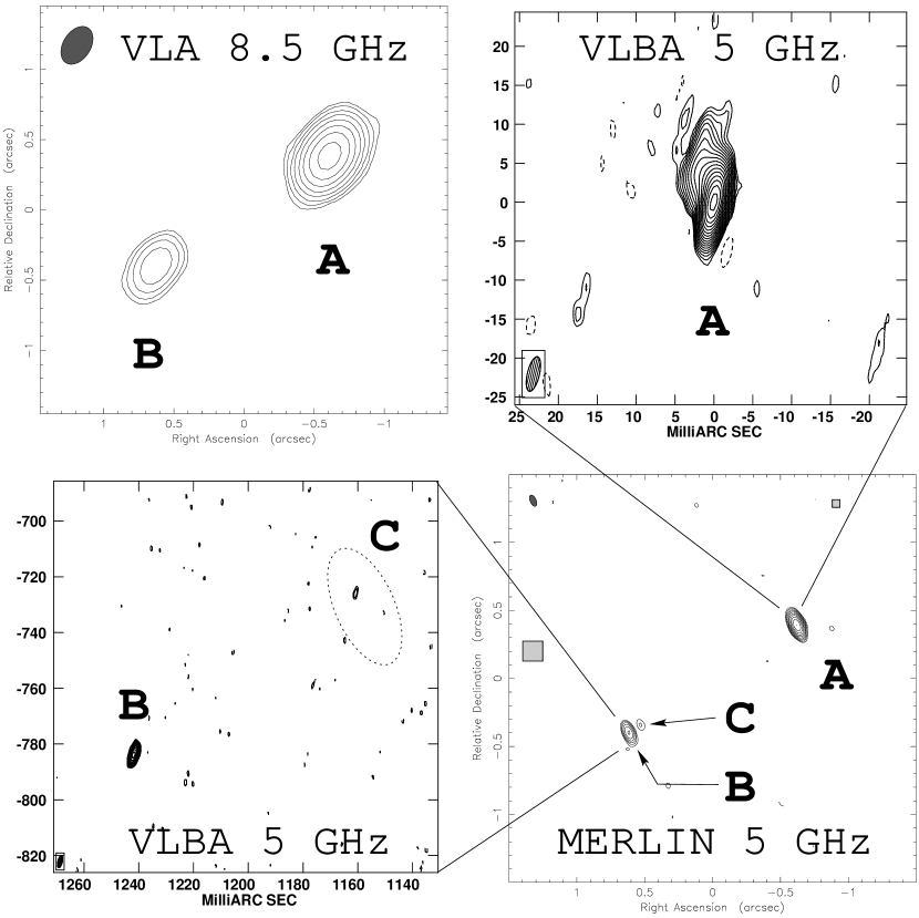
Figure 1: Radio contour maps of J1632–0033. In each panel, the synthesized beam is illustrated in one corner. Upper left. 8.5 GHz VLA observation of 1994 February 24. Contours begin at $3\sigma$ and increase by factors of two, where $\sigma=0.26$ mJy beam^-1. Lower right. 5 GHz MERLIN observation of 2001 April 13. Contours begin at $3\sigma$ and increase by factors of two, where $\sigma=0.13$ mJy beam^-1. The small gray squares illustrate the dimensions of the VLBA subimages centered on component A (upper right panel) and B+C (lower left panel). Upper right. From the 5 GHz VLBA observation of 2000 April 29. Contours begin at $3\sigma$ and increase by factors of $\sqrt{2}$, where $\sigma=0.13$ mJy beam^-1. Lower left. From the 5 GHz VLBA observation of 2000 April 29. Contours begin at $3\sigma$ and increase by factors of $\sqrt{2}$, where $\sigma=0.11$ mJy beam^-1. The dotted ellipse is centered on the MERLIN position of component C, and its dimensions are half the dimensions of the MERLIN synthesized beam.

Components A and B are unresolved in all the images except the VLBA image, in which component A is partially resolved. Component C is too faint to determine whether it is unresolved or slightly resolved with much confidence. Figure 1 displays a representative VLA image of the system, the deeper MERLIN image, and higher-resolution VLBA images of components A and B. Table 2 gives the relative positions of A, B, and C, as determined from the VLBA image. The J2000 coordinates of J1632–0033, as derived from the VLA observations, are also given in Table 2.

2.1 Data reduction and analysis

The details of the data reduction and analysis were as follows:

VLA: The VLA data were calibrated with standard routines in the software package AIPS. For the first three VLA observations (1984–1999), radio source 3C286 was used to set the absolute flux density scale, using the procedures recommended in the VLA Calibrator Manual. For the VLA observations in 2000, the source J2355+4950 was used instead; this compact source is monitored monthly by G. Taylor and S. Myers of NRAO, and has been found to have a stable flux density. The assumed flux densities of J2355+4950 were 2.306 Jy (1.4 GHz), 0.602 Jy (15 GHz), 0.473 Jy (22.5 GHz), and 0.284 Jy (43 GHz). We applied gain-elevation corrections for data at 15 GHz and higher frequencies based on gain curves prepared by NRAO staff.

Imaging and analysis were performed with the software package Difmap (Shepherd, Pearson, & Taylor, 1994). We fitted a surface-brightness model consisting of 2 unresolved points to the visibility function, and used this model to perform phase-only self-calibration with a solution interval of 30 seconds. This process, model-fitting and self-calibration, was repeated (typically 3 times) until the model converged. For the 1.4 GHz data, which had the lowest spatial resolution, we fixed the relative separation and orientation of the model components at the values obtained from the VLBA data.

ATCA: The ATCA data were calibrated using the software package MIRIAD (Sault, Teuben, & Wright, 1995). The absolute flux density scale of the ATCA data was set by observations of PKS B1934–638. The imaging and analysis steps were the same as for the VLA data. As with the 1.4 GHz VLA data, the relative separation of the two model components was kept fixed at the values derived from the VLBA data, in order to improve the accuracy with which we could extract separate flux densities for A and B.

MERLIN: Calibration of the MERLIN data was performed at Jodrell Bank using both standard MERLIN software and AIPS. The absolute flux scale was set by observing 3C286 and assuming a flux density of 7.38 Jy on the shortest baseline. Imaging and analysis were performed with Difmap in the same manner as for the VLA and ATCA data. For the second, much longer MERLIN observation, we also performed one round of amplitude self-calibration, with a solution interval of 30 minutes. In that case the residuals (after the two-component model was subtracted) indicated the presence of a third component. Our final model consisted of three point sources (A, B, and C).

VLBA: For the VLBA observation, the total observing bandwidth was divided into 4 intermediate frequency bands, each of which was subdivided into $16\times 0.5$ MHz channels. Fringe-fitting, calibration, and imaging of the VLBA data were all performed with AIPS. After fringe-fitting, we reduced the data volume by averaging in time into 6-second bins and in frequency into 1 MHz bins. These values were chosen to reduce the data volume as much as possible while keeping the amount of bandwidth smearing and time-average smearing below $1\%$ over the required field of view.

Components A and B were obvious in the “dirty” image (prior to deconvolution). We employed the multiple-field implementation of the CLEAN algorithm, with a 180 mas $\times$ 180 mas field centered on each component. The model developed by the CLEAN algorithm was used to self-calibrate the antenna phases with a solution interval of 30 seconds. We iterated this process 5 times before arriving at the final model. The images based on this model, with uniform weighting and an elliptical Gaussian restoring beam, are displayed in Figure 1.

After seeing component C in the MERLIN image, we repeated the imaging step using two 200 mas $\times$ 200 mas fields, one centered on component A, and the other centered between B and the expected location of C. We found a $4.5\sigma$ peak within 5 mas of the MERLIN position of C. It is the brightest peak within the field, and does not belong to the sidelobe pattern of either of the two brighter components A or B. We conclude that component C is also present in the VLBA image.

2.2 Radio observations—discussion

The flux densities of A, B, and C (when detected) are reported in Table 1 for each observation, along with the RMS noise level and an estimate of the uncertainty in the absolute flux scale. These numbers were used to generate the two plots presented in Figure 2.

The top panel of Figure 2 is a logarithmic plot of the total flux density of both components as a function of radio frequency. Evidently J1632–0033 has a fairly flat radio spectrum, typical of radio-loud quasars (and indeed, the optical spectrum presented in § 3.3 verifies that it is a quasar). From 5 GHz to 22.5 GHz, the data that were all taken in the year 2000 are a good match to the power law $S_{\nu}\propto\nu^{-0.3}$. At 8.5 GHz, there is evidence for variability at the 5–10% level on a time scale of years. (The discrepancies between the 5 GHz measurements are more difficult to interpret, because the VLBA and MERLIN probe much smaller angular scales than the other 5 GHz observations.)

Two compact, flat-spectrum radio components separated by $1\farcs 47$ are likely to be either a pair of quasars at the same redshift (a binary quasar) or a pair of gravitationally lensed images of a single quasar. In fact, J1632–0033 is a lens rather than a binary quasar. The most definitive evidence, optical detection of the lens galaxy, is presented in the next section. But, interestingly, lensing is implicated by the radio evidence alone.

The first clue is the near-equality of spectral indices of components A and B. This is a natural consequence of gravitational lensing, which is achromatic, but would require a coincidence under the binary quasar hypothesis. The bottom panel of Figure 2 is a logarithmic plot of the A/B flux density ratio as a function of frequency. The ratio increases by less than 30% over a factor of 30 in frequency (and even this may be due in part to components B and C being lumped together in the low-resolution images—see § 4.2). Assuming that component A obeys $S_{\nu}(A)\propto\nu^{\alpha}$, and likewise $S_{\nu}(B)\propto\nu^{\beta}$, then a least-squares analysis implies $\alpha-\beta=0.07\pm 0.01$. We estimate the probability of randomly drawing two quasars with spectral indices that match as closely to be 7%, by analyzing the histogram of spectral indices of flat-spectrum sources in the PMN tropical and equatorial catalogs.

The second piece of radio evidence, which is more compelling, is the location of the faint component C. It is located almost exactly where one would expect to find the center of a lens galaxy—along the line joining A and B, and closer to the dimmer of the two components, as simple lens models predict (see § 4.1). Regardless of whether C is emission from the lens galaxy or a third, demagnified image of the background quasar (see § 4.2), the existence and location of C implies that the system is a lens rather than a binary quasar.

3 Optical observations

3.1 HST images

On 2001 July 1 we obtained optical images of J1632–0033 with the WFPC2 camera aboard the HST. We obtained 3 dithered exposures through each of two filters, F555W ($\approx V$) and F814W ($\approx I$). The total exposure time for each filter was 2000 seconds. The target was centered in the PC chip.

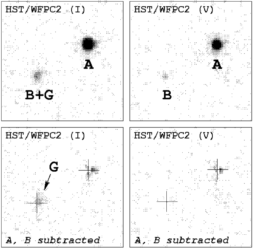
Figure 3: Top left panel. Optical image with HST/WFPC2 (F814W, $\approx I$ band). Bottom left panel. Same, after subtraction of a surface-brightness model consisting of two point sources (see § 3.1). Top right panel. Optical image with HST/WFPC2 (F555W, $\approx V$ band). Bottom right panel. Same, after subtraction of the two point sources from our final 3-component surface-brightness model (see § 3.1). The de Vaucouleurs profile has not been subtracted, in order to highlight the lens galaxy.

The exposures were combined and cosmic rays rejected using the Drizzle algorithm as implemented in IRAF. In both filters, light from a bright ($R=11$) binary star $30\arcsec$ to the south of J1632–0033 caused a large gradient in the background level across the PC chip, which was removed by fitting (and then subtracting) a second-order polynomial surface to the apparently empty regions of the image. The upper two panels of Figure 3 show the final images.

In the $V$-band image, the optical counterparts to radio components A and B were detected, and are unresolved. In the $I$-band image, A and B are also present, but there is a diffuse object near B that we identify as the lens galaxy. We constructed a photometric model for each image using software written by B. McLeod (see, e.g., Lehár et al. 2000). This program finds the parameters of a surface-brightness model (which consists of a user-determined number of point sources and simple galaxy profiles) convolved with a PSF computed by the program “Tiny Tim” (Krist & Hook, 1997), such that the mean-square residuals are minimized.

For the $I$-band image, we tried initially to fit a model consisting of 2 point sources only. Subtracting two point sources from the $I$-band image leaves behind residuals near A with peak intensity $\sim 3\%$ the central intensity of A, which in our experience is the level produced by inaccuracies in the Tiny Tim PSF. However, the residuals near B have peak values 40% the central intensity of B and $8\sigma$, where $\sigma$ is the RMS level in a blank region of the image. This indicates there is a diffuse source of unmodeled light near B: the lens galaxy.

Our final model consisted of two points and a circular de Vaucouleurs profile. Upon subtraction of this model, the residuals near B are consistent with random noise. In order to highlight the galaxy, the lower right panel of Figure 3 shows the image that results when only the point sources of the best-fit model have been subtracted. Table 3 lists the parameters of the best-fit photometric model.

As mentioned earlier, the position of the center of the galaxy derived from the HST image is consistent with the location of radio component C, and both are located where simple lens models predict that a lens galaxy (or demagnified third image) to appear. However, because it is not clear whether the galaxy itself is responsible for the radio emission, we have labeled the optical galaxy G rather than C.

For the $V$-band image, our model consisted of two point sources. The residuals (after the best-fit model was subtracted from the original image) are shown in the lower left panel. The peak residuals near A are 3–5% of the central intensity of A. The peak residuals near B are dominated by noise rather than PSF subtraction; they are $3\sigma$ where $\sigma$ is the RMS level in a blank region of the image. The separation and position angle of the points are consistent with the A/B radio values.

For the final $V$-band results listed in Table 3, we also added a de Vaucouleurs profile to the model, but we fixed its effective radius and fixed all the positions of the model components at the $I$-band values, and allowed only their fluxes to vary. Because the $V$-band image does not provide independent evidence for the galaxy, the $V$-band galaxy magnitude should probably be considered as an approximate lower limit.

The zero-points of the magnitude scales were 21.69 for $I$ and 22.54 for $V$, as determined by Dolphin (2000) and corrected for infinite aperture. We also applied a correction for losses due to the charge-transfer-efficiency problem of WFPC2, as per the prescription of Dolphin (2000). These corrections were large: for component A they were $+0.20$ mag for both filters, and for components B+G they were $+0.50$ for $I$ and $+0.90$ for $V$. The quoted magnitudes are therefore considerably uncertain and should be treated with caution.

3.2 Ground-based images

Before obtaining the HST image we attempted to search for evidence of a lens galaxy in ground-based optical images. Although the HST image contains the most convincing evidence of the lens galaxy, the ground-based results are useful in providing total magnitudes and flux ratios over a wider range of wavelengths.

On 2000 July 25 we obtained $BVRI$ optical images of J1632–0033 with the Mosaic II camera on the prime focus of the Blanco 4-meter telescope at CTIO. The night was photometric. Each exposure lasted 600 seconds. After extracting the images from chip #2, we corrected them for cross-talk from the paired amplifier, bias-subtracted and flat-fielded them with standard IRAF procedures, and defringed the $I$-band images using a fringe template kindly supplied by R.C. Dohm-Palmer.

The seeing was $1\farcs 2$. The object could barely be resolved in the $I$-band image but appeared pointlike in the other images. A synthetic circular aperture of radius $7\arcsec$ was used to compute total instrumental magnitudes (after subtracting all neighboring objects within $14\arcsec$). To place the instrumental magnitudes on a standard photometric system, we also observed the standard stars #355, #360, and #361 from field SA110 described by Landolt (1992). Our photometric solutions took the form:

$$m_{\mbox{std}}=m_{\mbox{inst}}+c_{1}+c_{2}(B_{\mbox{inst}}-R_{\mbox{inst}}),$$ (1)

where

$$m_{\mbox{inst}}=-2.5\log\left(\frac{\mbox{counts}}{\mbox{time}}\right)-k_{m}\times{\mbox{airmass}}.$$ (2)

We adopted “typical” CTIO coefficients of $k_{I}=0.06$, $k_{R}=0.11$, $k_{V}=0.15$, and $k_{B}=0.28$ (Landolt, 1992). Star #355 was not used for the $I$-band solution because it was overexposed. Table 4 reports the calibrated magnitudes of J1632–0033. The $I$-band magnitude disagrees with the F814W magnitude reported in § 3.1, possibly due to the CTE problem of WFPC2.

On 25–26 March 2001 we obtained optical images of J1632–0033 with MagIC, a CCD camera at the Nasmyth focus of the 6.5-meter Baade telescope. We obtained 480-second exposures in each of the Sloan filters $g^{\prime}$, $r^{\prime}$, and $i^{\prime}$ in $0\farcs 8$ seeing. On 11–12 June 2001 we also obtained an additional three $i^{\prime}$ exposures totaling 1350 seconds, in $0\farcs 6$ seeing.

The optical counterpart of J1632–0033 appeared double in all images. In particular, in the $i^{\prime}$-images from June, the southeast component was slightly resolved rather than pointlike, as would be expected from a combination of quasar B and the lens galaxy.

For each filter, we estimated the flux ratio A:(B+G) using the following procedure. With the DAOPHOT package in IRAF, we constructed an empirical PSF of radius $3\arcsec$, using the signal-weighted average of several bright and isolated field stars. We then fit a model consisting of two point sources to the optical counterpart of J1632–0033. The results for the flux ratio are printed in Table 5.

The ratio decreases with wavelength for two reasons. First, G is redder than the quasar images, as demonstrated by the analysis of the HST images in § 3.1. Second, the reddening of the quasar light due to passage through the lens galaxy is apparently larger for image B than for image A. This follows from the observation that the flux ratios in the $g^{\prime}$ and $V$-band images (which do not contain a significant contribution from lens galaxy light) are larger than the radio value. This is reasonable, since B is considerably closer to the galaxy center than A.

3.3 Optical spectrum

On 2000 September 1, we obtained an optical spectrum of J1632–0033 with the 3.5-meter telescope at Apache Point Observatory. We used the Double Imaging Spectrograph in low resolution mode. The processed spectrum had a very weak signal, with two features at the $1-2\sigma$ level whose wavelength ratio was consistent with the common quasar emission lines Ly$\alpha$ (1216Å) and C IV (1549Å), allowing the tentative identification of J1632–0033 as a quasar at redshift 3.42.

This identification was confirmed on 2001 March 23, when we obtained an optical spectrum with the 6.5-meter Baade telescope. We used a Boller & Chivens slit spectrograph with a 600 lines mm^-1 grating, giving a pixel scale of $0\farcs 44$ pixel^-1, dispersion 2.75Å pixel^-1, resolution $10$Å, and wavelength coverage 4500–7300Å. We used the WG360 Schott glass blocking filter to block second order contamination. The slit was $1\farcs 3$ wide, centered on component A, and oriented perpendicular to the A/B position angle.

Flat-fielding, spectrum extraction, and wavelength calibration were carried out with standard IRAF procedures. The processed spectrum is shown in Figure 4. Here the Ly$\alpha$ and C IV emission lines are detected with high significance, implying $z=3.424\pm 0.007$. The expected position of Si IV + O IV] (1400Å) is also shown.

As for the lens galaxy, its redshift is currently unknown, but it is possible to estimate photometrically. Kochanek et al. (2000) devised a method to estimate the redshift of a lens galaxy, given the redshift of the background source, the image separation, and the magnitudes and effective radius of the galaxy. The idea is to require that the galaxy properties are consistent with the passively-evolving fundamental plane (FP) of early-type galaxies. In this case the FP estimate of the lens redshift is $z=1.0\pm 0.1$.

4 Gravitational lens models

4.1 Simple two-image models

Constructing a model of the gravitational potential of the lens galaxy is important for three reasons. First, if the model is physically plausible, it corroborates our claim that J1632–0033 is truly a lens. Second, a lens model is required to predict the time delay between lensed images as a function of the Hubble constant. Third, if enough constraints are available, the lens model may reveal interesting aspects of the matter distribution of the lens galaxy, including dark matter.

The present observations of J1632–0033 provide five constraints on models of the lens potential: the positions of A and B with respect to the lens center, and the A/B radio flux density ratio. The relative separation of A and B is known precisely from the VLBA image. Because the position of radio component C is consistent with the optical lens galaxy G, we assume that C marks the lens center, although we enlarge the uncertainty to 10 mas to allow for the possibility of a small displacement between the lens center and the radio component. Our measurements of the radio flux density ratio have a mean of 13.2, and a scatter of 15%.

The simplest plausible lens model is a singular isothermal sphere, which produces two images on opposite sides of the lens, with a magnification ratio equal to the ratio of distances from each image to the lens center. As stated earlier in §§ 2.2 and 3.1, the present data are nearly consistent with this model. Component C lies only 7 mas from the line joining A and B, and the ratio of distances is $13.8\pm 0.8$, in agreement with the flux density ratio.

This confirms that gravitational lensing is a natural explanation for the morphology of J1632–0033. Unfortunately there are not enough constraints to explore less idealized lens models in detail. A singular isothermal ellipsoid (SIE), for example, has five parameters (the position of the lens, the mass scale, the ellipticity and the position angle), and is therefore uniquely determined by our five constraints. Table 6 gives the parameters of the SIE model, as computed with lens modeling software written by Keeton (2001). The quoted uncertainties reflect the variations in the parameters obtained by varying the position of the lens center and the magnification ratio throughout their quoted error ranges.

The final quantity listed in Table 6, labeled $\Delta\tau$, is a dimensionless factor that may be converted into a time delay $\Delta t$ by assuming a lens redshift and a cosmological model as follows:

$$\Delta t=\frac{D_{l}D_{s}}{2cD_{ls}}(1+z_{l})\Delta\tau.$$ (3)

In this equation, $z_{l}$ is the lens redshift, and $D_{l}$, $D_{s}$ and $D_{ls}$ are the angular-diameter distances to the lens, to the source, and between the lens and source, respectively.

If we assume $z_{l}=1.0\pm 0.1$, as predicted by the FP method (see § 3.3), then in a cosmology in which matter is distributed smoothly with $\Omega_{\mathrm{m}}=0.3$ and $\Omega_{\Lambda}=0.7$, the result is $h\Delta t=118.5\pm 1.9$ days, where $H_{0}=100h$ km s^-1 Mpc^-1 as usual. If instead $\Omega_{\mathrm{m}}=0.3$ and $\Omega_{\Lambda}=0$, then $h\Delta t=125.7\pm 2.0$ days. Image A is expected to lead image B. The uncertainties quoted here are internal to the SIE model only; the true uncertainty in the time delay is much larger.

4.2 The nature of component C

We now return to the question of the origin of C, the third and faintest radio component. Its position relative to A and B agrees with that of the galaxy G detected in the $I$-band HST image (§ 3.1), so it possibly represents emission from a faint AGN in the lens galaxy. In this section we consider the implications of another possibility—that C represents a third quasar image.

Although the SIS and SIE models only predict two images of the background source, many lens models predict the existence of a third image of the quasar located close to the lens center that is demagnified by an amount depending on the central surface density of the lens galaxy (see, e.g., Narasimha, Subramanian, & Chitre 1986). The existence or absence of the “odd image” can therefore provide information on the central structure of the lens galaxy, which would otherwise be very difficult to obtain for a galaxy at $z\sim 1$. The only lens for which an odd image has been identified confidently is APM 08279+5255 (Ibata et al., 1999; Egami et al., 2000). Many of the current observations of radio lenses, which have typical dynamic ranges of 100–1000, show no evidence for odd images; presumably the absence of the odd images is due to the high central surface densities of the lens galaxies (Wallington & Narayan, 1993; Rusin & Ma, 2001; Keeton, 2001b).

There are two simple extensions of singular isothermal lens models that produce three images. In the first category are models with a finite core radius $r_{c}$. In these models, the magnification of the odd image is approximately $(\theta_{c}/\theta_{E})^{2}$, where $\theta_{E}$ is the Einstein ring radius of the lens galaxy (approximately half the image separation), and $\theta_{c}=D_{l}r_{c}$, the angle subtended by the core radius. In our SIE model for J1632–0033, if C is an odd image then its magnification is $(111\pm 37)^{-1}$, implying $(\theta_{c}/\theta_{E})=0.095\pm 0.016$. For $z_{l}=1$ this corresponds to a core radius of $590\pm 100$ parsecs. A core radius this large would be interesting, because one would expect much smaller (or zero) core radii based on the cusped distribution of starlight in HST images of nearby galaxies (Faber et al., 1997), the absence of odd images of most other lensed quasars (Wallington & Narayan, 1993; Rusin & Ma, 2001; Keeton, 2001b), and theoretical simulations of cold-dark-matter haloes (Navarro, Frenk, & White, 1996).

For exactly these reasons, several authors have recently emphasized a second category of lens models, which have a central density cusp (see, e.g., Evans & Wilkinson, 1998; Keeton, 2001b; Muñoz, Kochanek, & Keeton, 2001). If the cusp in the three-dimensional mass density obeys the power law $\rho\sim r^{-\gamma}$ for small $r$, then a third image is produced for $\gamma<2$. These models have even more trouble accomodating C as an odd image. For example, Muñoz, Kochanek, & Keeton (2001) applied a cusped lens model to the 3-image lens APM 08279+5255, and found that, in order to match the observational constraints, the cusp exponent had to be so shallow as to approach the limit of models with a finite core radius.

In short, if C is a third quasar image, then the mass distribution of the inner few hundred parsecs of the lens galaxy in J1632–0033 is not as centrally condensed as one would expect from studies of nearby galaxies, studies of other lenses, and theoretical models of halo formation. It would therefore be interesting to test definitively whether C is galaxy emission or a third quasar image.

Probably the simplest approach would be to measure the radio continuum spectrum of C over as broad a wavelength range as possible. If C is a third image, its spectrum should match that of A and B. There is one indication in the present data that C may have a steeper spectrum than that of A and B: the trend of increasing flux density ratio with radio frequency that is depicted in the bottom panel of Figure 2. The VLA data below 22.5 GHz do not have sufficient angular resolution to distinguish B and C, so their flux densities are lumped together in the models. A steeper spectrum for C would therefore cause the inferred flux density ratio to decrease with frequency. For example, if the true A/B flux density ratio is 14.7 (as implied by the April 2001 MERLIN data) and independent of frequency, then in order to lower the flux density ratio to match the 1.4 GHz data, the required spectral index of C is $\alpha=-1.3$.

Unfortunately there are other reasons to expect that the measured flux density ratio A/B is not completely independent of frequency, such as variability (coupled with the time delay), and the possibility of a large magnification gradient across a source with frequency-dependent substructure. It would be preferable to obtain multi-wavelength radio images with sufficient angular resolution and sensitivity to resolve all three components.

5 Summary and future prospects

Radio source J1632–0033 is the fourth confirmed gravitational lens in our survey of the southern sky for new lenses. Here we briefly review the evidence for lensing and the immediate prospects for using this lens to obtain interesting astrophysical information. Two compact, flat-spectrum radio components separated by $1\farcs 47$ are almost certainly either a binary quasar or a pair of lensed images of a single quasar. The flux density ratio is within 15% of 13.2 as measured from 1.4 GHz to 43 GHz; this similarity of radio spectra favors the lens hypothesis. The lens galaxy is apparent in an optical image with HST, and it is located exactly where one would expect, based on the simplest plausible lens model.

The background source is a spectroscopically verified quasar at redshift 3.42. The optical magnitude, color, and effective radius of the lens galaxy (together with the mass estimate provided by the image separation) are consistent with a passively-evolving elliptical galaxy at redshift unity. There is a faint third radio component located at or near the center of the lens galaxy, which is either faint emission from the galaxy itself, or a third quasar image. In the latter case, the study of the faint component may be useful as a probe of the central few hundred parsecs of a $z\sim 1$ galaxy.

The flat radio spectrum, and mild variability observed at 8.5 GHz, make this system a candidate for flux monitoring, in order to use the time delay between the quasar images to determine the Hubble constant. The present data, however, do not provide nearly enough model constraints for this method to be competitive with local distance-scale methods. One would need an additional, rich body of constraints, possibly from infrared imaging of the quasar host galaxy (see, e.g. Kochanek, Keeton, & McLeod, 2001) or VLBI substructure (see, e.g., Trotter, Winn & Hewitt, 2000).

Figure 2: Top panel. Total flux density of J1632–0033 as a function of radio frequency. For reference, a power law $S_{\nu}\propto\nu^{-0.3}$ is also plotted.
Bottom panel. Flux density ratio as a function of radio frequency. The error estimates were computed by assuming that the uncertainty in the relative flux density scale is equal to the RMS noise level in the image.

Figure 4: Optical spectrum of component A of J1632–0033 (see § 3.3), with resolution $\sim 10$Å. The redshift is $z=3.424\pm 0.007$.

Table 1: Radio observations of J1632–0033

Date	Observatory	Frequency	Bandwidth	Duration	Beam FWHM	Flux density			RMS noise	Abs. flux
		(GHz)	(MHz)	(min)	(mas $\times$ mas, P.A.)	A (mJy)	B (mJy)	C (mJy)	(mJy/beam)	uncertainty
1984 Dec 17	VLA	4.860	100	1.3	$496\times 393$ ($-34\arcdeg$)	206.01	17.06	$\cdots$	0.38	5%
1994 Feb 24	VLA	8.452	50	1.3	$294\times 198$ ($-33\arcdeg$)	152.53	12.48	$\cdots$	0.26	3%
1999 Jun 30	VLA	8.440	100	1.5	$743\times 207$ ($54\arcdeg$)	138.90	12.21	$\cdots$	0.27	5%
2000 Apr 05	MERLIN	4.994	15	110	$95\times 42$ ($23\arcdeg$)	177.41	13.80	$<2.9$	0.57	5%
2000 Apr 29	VLBA	4.987	32	54	$3.4\times 1.4$ ($-2\arcdeg$)	166.21	11.93	0.50	0.14	5%
2000 Sep 26	ATCA	4.800	128	5	$1385\times 9840$ ($0\arcdeg$)	216.62	16.48	$\cdots$	0.57	3%
2000 Sep 26	ATCA	6.080	128	10	$1140\times 2600$ ($0\arcdeg$)	186.44	14.29	$\cdots$	0.43	3%
2000 Sep 26	ATCA	8.640	128	15	$791\times 2020$ ($0\arcdeg$)	164.18	12.56	$\cdots$	0.43	3%
2000 Nov 11	VLA	1.425	100	2.0	$3430\times 1250$ ($53\arcdeg$)	211.35	18.68	$\cdots$	0.30	5%
2000 Nov 11	VLA	14.940	100	10	$242\times 120$ ($52\arcdeg$)	143.81	9.42	$<1.5$	0.29	5%
2000 Nov 11	VLA	22.460	100	10	$184\times 78$ ($54\arcdeg$)	126.48	8.36	$<3.7$	0.74	10%
2000 Dec 24	VLA	42.640	100	12	$62\times 38$ ($-44\arcdeg$)	83.42	5.43	$<3.3$	0.66	15%
2001 Apr 13	MERLIN	4.994	15	525	$88\times 44$ ($24\arcdeg$)	208.12	14.20	0.87	0.13	5%

Table 2: VLBA relative positions

Component	$\Delta$R.A. ($x-x_{\mathrm{A}}$)	$\Delta$Decl. ($y-y_{\mathrm{B}}$)
	(mas)	(mas)
A	$\cdots$	$\cdots$
B	$-1241.6\pm 0.1$	$-784.6\pm 0.2$
C	$-1160.6\pm 0.7$	$-726.8\pm 1.7$

Note. — The J2000 coordinates of component A are R.A. $=16^{\mathrm{h}}32^{\mathrm{m}}57\fs 680$, Decl. $=-00\arcdeg 33\arcmin 21\farcs 05$, within $0\farcs 15$.

Table 3: Photometric model of J1632–0033 based on HST/WFPC2 images

Component	$\Delta x$	$\Delta y$	$R_{\mbox{eff}}$	$m_{\mbox{F555W}}$	$m_{\mbox{F814W}}$
	(mas)	(mas)	(arcsec)
A	0	0	$\cdots$	$21.67\pm 0.06$	$20.74\pm 0.06$
B	$-1242.8\pm 3$	$-790.9\pm 3$	$\cdots$	$24.97\pm 0.23$	$24.4\pm 0.1$
G	$-1161.6\pm 9$	$-737.8\pm 9$	$0.20\pm 0.08$	$\geq 25.5$	$23.3\pm 0.2$

Note. — Quoted uncertainties are based on statistical error only, and are internal to the chosen model-fitting procedure. In particular the magnitude uncertainties do not include the overall uncertainty in the zero-point or CTE correction (see § 3.1).

Table 4: Total optical magnitudes of J1632–0033

Filter	Magnitude
$B$	$22.85\pm 0.10$
$V$	$21.29\pm 0.05$
$R$	$20.99\pm 0.05$
$I$	$20.36\pm 0.10$

Table 5: Optical flux ratios

Filter	A:(B+G)
$g^{\prime}$	$27\pm 8$
$r^{\prime}$	$24\pm 3$
$i^{\prime}$	$11.5\pm 0.9$

Table 6: SIE model parameters

Parameter	Value
Einstein ring radius, $b$	$0\farcs 731\pm 0.015$
Ellipticity, $\epsilon$	$0.078^{+0.12}_{-0.02}$
Position angle	$-4\arcdeg^{+70}_{-28}$
$x_{\mbox{source}}-x_{\mbox{A}}$	$-0\farcs 633\pm 0\farcs 024$
$y_{\mbox{source}}-y_{\mbox{A}}$	$-0\farcs 374\pm 0\farcs 030$
Magnification of A	$2.11\pm 0.17$
$\Delta\tau$	$0.932\pm 0.015$

Note. — Quoted uncertainties reflect the range in parameter values obtained by varying (separately) the lens position by 10 mas and the magnification ratio by 15%.

References

- Blandford & Narayan (1992) Blandford, R.D. & Narayan, R. 1992, ARA&A, 30, 311
- Browne & Myers (2000) Browne, I.W.A. & Myers, S. 2000, to appear in New Cosmological Data and the Values of the Fundamental Parameters, Proc. IAU Symposium 201, Manchester, England
- Chen & Hewitt (1993) Chen, G. & Hewitt, J.N. 1993, AJ, 106, 1719
- Condon et al. (1998) Condon, J.J., Cotton, W.D., Greisen, E.W., Yin, Q.F., Perley, R.A., Taylor, G.B., & Broderick, J.J. 1998, AJ, 115, 1693
- Dolphin (2000) Dolphin, A.E. 2000, PASP. 112, 1397
- Egami et al. (2000) Egami, E., Neugebauer, G., Soifer, B.T., Matthews, K., Ressler, M., Becklin, E.E., Murphy, T.W. Jr., & Dale, D.A. 2000, ApJ, 535, 561
- Evans & Wilkinson (1998) Evans, N.W. & Wilkinson, M.I. 1998, MNRAS, 296, 800
- Faber et al. (1997) Faber, S. et al. 1997, AJ, 114, 1771
- Falco et al. (1998) Falco, E.E., Kochanek, C.S., & Muñoz, J.A. 1998, ApJ, 494, 47
- Falco et al. (1999) Falco, E.E., Impey, C.D., Kochanek, C.S., Lehár, J., McLeod, B.A., Rix, H.-W., Keeton, C.R., Muñoz, J.A., & Peng, C.Y. 1999, ApJ, 523, 617
- Fukugita, Futamase & Kasai (1990) Fukugita, M., Futamase, T., & Kasai, M. 1990, MNRAS, 246, 24
- Griffith & Wright (1993) Griffith, Mark R. & Wright, Alan E. 1993, AJ, 105, 1666
- Ibata et al. (1999) Ibata, R.A., Lewis, G.F., Irwin, M.J., Lehár, J., & Totten, E.J. 1999, AJ, 118, 1922
- Keeton (2001) Keeton, C.S. 2001, preprint (astro-ph/0102340)
- Keeton (2001b) Keeton, C.S. 2001, preprint (astro-ph/0105200)
- King et al. (1998) King, Lindsay J., Browne, Ian W.A., Marlow, Daniel R., Patnaik, Alok R., & Wilkinson, Peter N. 1998, MNRAS, 307, 225
- Kochanek (1995) Kochanek, C.S. 1995, ApJ, 445, 559
- Kochanek et al. (2000) Kochanek, C.S., Falco, E.E., Impey, C.D., Lehár, J., McLeod, B.A., Rix, H.-W., Keeton, C.R., Muñoz, J.A., & Peng, C.Y. 2000, ApJ, 543, 131
- Kochanek, Keeton, & McLeod (2001) Kochanek, C.S., Keeton, C.R., & McLeod, B.A. 2001, ApJ, 547, 50
- Koopmans & Fassnacht (1999) Koopmans, L. & Fassnacht, C. 1999, ApJ, 527, 513
- Krist & Hook (1997) Krist, J.E. & Hook, R.N. 1997, The Tiny Tim User’s Guide, version 4.4 (Baltimore: STScI)
- Landolt (1992) Landolt, A.U. 1992, AJ, 104, 340
- Lawrence et al. (1986) Lawrence, C.R., Bennett, C.L., Hewitt, J.N., Langston, G.I., Klotz, S.E., Burke, B.F., & Turner, K.C. 1986, ApJS, 61, 105
- Lehár et al. (2000) Lehár, J., Falco, E.E., Kochanek, C.S., McLeod, B.A., Muñoz, J.A., Impey, C.D., Rix, H.-W., Keeton, C.R., & Peng, C.Y. 2000, ApJ, 536, 584
- Muñoz, Kochanek, & Keeton (2001) Muñoz, J.A., Kochanek, C.S., & Keeton, C.R. 2001, preprint (astro-ph/0103009)
- Narasimha, Subramanian, & Chitre (1986) Narasimha, D., Subramanian, K., & Chitre, S.M. 1986, Nature, 321, 45
- Narayan (1998) Narayan R. 1998, New Astronomy Reviews, 42, 73
- Navarro, Frenk, & White (1996) Navarro, J.F., Frenk, C.S., & White, S.D.M. 1997, ApJ, 490, 493
- Refsdal (1964) Refsdal, S. 1964 MNRAS, 128, 307
- Rusin & Ma (2001) Rusin, D. & Ma, C.-P. 2001, ApJ, 549, 33
- Sault, Teuben, & Wright (1995) Sault R.J., Teuben P.J., & Wright M.C.H. 1995, in Astronomical Data Analysis Software and Systems IV, eds. R. Shaw, H.E. Payne, J.J.E. Hayes, ASP Conf. Ser., 77, 433-436.
- Shepherd, Pearson, & Taylor (1994) Shepherd, M.C., Pearson, T.J., & Taylor, G.B. 1994, BAAS, 26, 987
- Trotter, Winn & Hewitt (2000) Trotter, Catherine S., Winn, Joshua N., & Hewitt, Jacqueline N. 2000, ApJ, 535, 671
- Turner (1990) Turner, E. 1990, ApJ, 365L, 43
- Wallington & Narayan (1993) Wallington, S. & Narayan, R. 1993, ApJ, 403, 517