Quantum Field Theoretic Description of Matter in the Universe

Abstract

Quantum field theory at finite temperature and density can be used for describing the physics of relativistic plasmas. Such systems are frequently encountered in astrophysical situations, such as the early Universe, Supernova explosions, and the interior of neutron stars. After a brief introduction to thermal field theory the usefulness of this approach in astrophysics will be exemplified in three different cases. First the interaction of neutrinos within a Supernova plasma will be discussed. Then the possible presence of quark matter in a neutron star core and finally the interaction of light with the Cosmic Microwave Background will be considered.

I Introduction

The interaction of elementary particles with a medium in equilibrium or out of equilibrium can be described by applying quantum field theory at finite temperature $T$, chemical potential $\mu$, or in non-equilibrium. Using perturbation theory, self energies, scattering amplitudes, the free energy, etc. can be calculated. In this way effective masses, Debye screening, dispersion relations, refractive indices, damping, decay and production rates, the equation of state and other interesting properties of the interacting particle and the medium can be derived. Famous examples are listed below.

• Effective in-medium neutrino masses, which lead to the MSW-effect, can be derived from the neutrino self energy at finite temperature and density [15].

• The plasmon effect, which describes the decay of an in-medium photon (plasmon) in a stellar plasma into a neutrino pair, $\gamma\rightarrow\nu\bar{\nu}$, provides an effective energy loss mechanism for hot and dense stars [1]. In a relativistic plasma the use of thermal field theory increases the emissivity by about a factor of 3 [5] compared to previous approaches.

• The baryon asymmetry of the Universe can be generated by the sphaleron decay during the electroweak phase transition. For calculating the sphaleron decay rate in the early Universe a new method in finite temperature field theory has been developed [6].

After a brief introduction to some basic concepts of thermal field theory, three examples of its application to astrophysical problems are discussed: neutrino interactions in a Supernova plasma, strange quark matter in neutron stars and as a dark matter candidate, and the interaction of light with the Cosmic Microwave Background.

II Thermal Field theory

Perturbative field theory at finite temperature or density is based either on the so-called imaginary (ITF) or real time formalism (RTF) (see e.g. [20]). As a simple example for illustrating these methods we will discuss the $\phi^{4}$-theory at finite temperature briefly. The most important quantity in perturbative field theory is the Feynman propagator. At zero temperature it is defined as the vacuum expectation value of the time-ordered product of two field operators. At finite temperature the vacuum expectation value has to be replaced by a thermal expectation value containing a sum over all thermally excited states. Using the plane-wave expansion of the fields and the canonical ensemble one gets [20]

$$i\>\Delta_{F}^{T>0}(x-y)=\frac{1}{Z}\>\sum_{n}\>\langle n|{\cal T}\{\phi(x)\phi(y)\}|n\rangle\>e^{-E_{n}/T}$$ (1)

$${\buildrel x_{0}>y_{0}\over{=}}\int\frac{d^{3}k}{(2\pi)^{3}}\>\frac{1}{2\omega_{k}}\>\left\{[1+n_{B}(\omega_{k})]\>e^{-iK(x-y)}+n_{B}(\omega_{k})\>e^{iK(x-y)}\right\},$$ (2)

where $Z$ is the partition function and $n_{B}(\omega_{k})=1/[\exp{(\omega_{k}/T)}-1]$ the Bose-Einstein distribution with $\omega_{k}^{2}=k^{2}+m^{2}$. Here we use the notation $K^{2}=k_{0}^{2}-k^{2}$, $k=|{\bf k}|$. This expression has a simple physical interpretation. At $T=0$ the propagator describes the creation of a scalar particle at the space-time point $y$ (for $x_{0}>y_{0}$) and its propagation to $x$, where it is destroyed. At finite temperature there is besides spontaneous creation at $y$, given by the term 1 in the square brackets, also induced emission and absorption proportional to $n_{B}(\omega_{k})$ due to the presence of the heat bath.

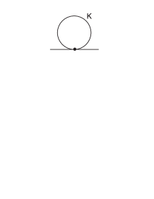
FIG. 1.: Tadpole diagram

In the ITF the propagator given above can be expressed as a sum over discrete, imaginary energies (Matsubara frequencies), $k_{0}=2\pi inT$,

$$i\>\Delta_{F}^{T>0}(x-y)=iT\>\sum_{k_{0}}\int\frac{d^{3}k}{(2\pi)^{3}}\>\frac{i}{K^{2}-m^{2}}\>e^{-iK\cdot(x-y)}.$$ (3)

The ITF will be exemplified by calculating the simplest self energy in the scalar theory, namely the tadpole diagram shown in Figure 1.

Modifying the standard Feynman rules by summing over $k_{0}$ instead of integrating we find

$$\Pi = \frac{i}{2}\>(-i\,4!\,g^{2})\>iT\>\sum_{k_{0}}\int\frac{d^{3}k}{(2\pi)^{3}}\>i\>\frac{1}{K^{2}-m^{2}}$$ (4)

$$= 6\>g^{2}\>\int\frac{d^{3}k}{(2\pi)^{3}}\>\frac{1}{\omega_{k}}\>[1+2n_{B}(\omega_{k})],$$ (5)

where $g^{2}$ is the coupling constant associated with the vertex of the $\phi^{4}$-theory. In the massless case, $m=0$, the integral in (5) can be done exactly, leading to the simple result $\Pi=g^{2}T^{2}$.

From the self energy we can construct an effective, in-medium propagator by using the Dyson-Schwinger equation, $\Delta^{*}=\Delta+\Delta\Pi\Delta^{*}$, yielding

$$\Delta^{*}=\frac{1}{K^{2}-m^{2}-\Pi}.$$ (6)

This propagator agrees with the bare one if the bare mass, $m$, is replaced by the effective mass $M=\sqrt{m^{2}+\Pi}$. The dispersion relation of the scalar field in the medium follows from the poles of the effective propagator: $\omega=\sqrt{k^{2}+M^{2}}$.

An alternative method to the ITF is the RTF, where the thermal propagator in momentum space is given by

$$i\>\Delta(K)=\frac{i}{K^{2}-m^{2}+i\epsilon}+2\>\pi\>n_{B}(|k_{0}|)\>\delta(K^{2}-m^{2}).$$ (7)

In order to avoid unphysical singularities from products of $\delta$-functions, which can appear in diagrams with two propagators, the propagator has been extended to a $2\times 2$-matrix [13]. An important advantage of the RTF compared with the ITF is the possible generalization to non-equilibrium by replacing the equilibrium distribution in (7) by a non-equilibrium.

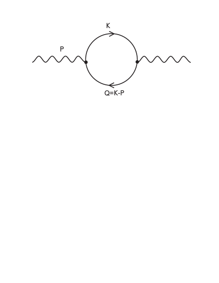
FIG. 2.: QED Polarization tensor containing an electron-positron loop

Now we will turn to gauge theories (QED, QCD, electroweak theory) at finite temperature and density, which are relevant for astrophysical situations. As an important example we consider the one-loop QED polarization tensor in an electron-positron plasma shown in Figure 2.

In contrast to the tadpole diagram the polarization tensor is energy and momentum dependent. It can be calculated exactly only in the high-temperature limit which is equivalent to the Hard-Thermal-Loop (HTL) limit, in which the loop momentum is assumed to be much larger than the external momentum. The high-temperature limit corresponds to an ultrarelativistic electron-positron plasma as it exists in Supernovae. Due to the breaking of Lorentz invariance by choosing the frame of the heat bath, the polarization tensor has two independent components, for which we take the longitudinal and the transverse. In the HTL limit they read

$$\Pi_{L}(p_{0},p) = -3\,m_{\gamma}^{2}\left(1-\frac{p_{0}}{2p}\ln\frac{p_{0}+p}{p_{0}-p}\right),$$ (8)

$$\Pi_{T}(p_{0},p) = \frac{3}{2}\,m_{\gamma}^{2}\>\frac{p_{0}^{2}}{p^{2}}\>\left[1-\left(1-\frac{p^{2}}{p_{0}^{2}}\right)\>\frac{p_{0}}{2p}\>\ln\frac{p_{0}+p}{p_{0}-p}\right],$$ (9)

where $m_{\gamma}^{2}=e^{2}T^{2}/9$ can be regarded as a thermal photon “mass”. However, it should be noted that this mass does not break gauge invariance.

By resumming the polarization tensor using the Dyson-Schwinger equation we construct an effective photon propagator which describes the propagation of collective photon modes (plasmons) in a QED plasma. The corresponding dispersion relations for the longitudinal and the transverse plasma waves are shown in Figure 3.

FIG. 3.: Dispersion relations of longitudinal and transverse photons in a QED plasma

Finally, let me mention that in the case of two-loop self energies, from which e.g. damping rates follow, infrared singularities and gauge dependent results (“plasmon puzzle”) are encountered. Braaten and Pisarski [4] developed a method, the HTL resummation technique, for avoiding these problems, which allows a consistent treatment of gauge theories at finite temperature.

III Neutrino Interactions in Supernovae

Neutrinos are copiously emitted from the core of a Supernova. They interact with the surrounding plasma, providing an effective mechanism for energy deposition, which pushes the shock wave outwards and finally triggers the explosion [8]. Important neutrino interaction processes in the plasma are $\nu e^{\pm}\leftrightarrow\nu e^{\pm}$, $\bar{\nu}e^{\pm}\leftrightarrow\bar{\nu}e^{\pm}$, and $\nu\bar{\nu}\leftrightarrow e^{+}e^{-}$.

The differential rate for instance for $\nu\bar{\nu}$-annihilation is given by

$$\frac{dR_{\nu\bar{\nu}}}{d^{3}q_{1}d^{3}q_{2}}=\frac{1}{2q_{1}2q_{2}}\frac{1}{1-e^{-E/T_{e}}}M^{\mu\nu}\>{\rm Im}\{\Pi_{\mu\nu}(Q_{1}+Q_{2})\},$$ (10)

where

$$M^{\mu\nu}=8(Q_{2}^{\mu}Q_{1}^{\nu}+Q_{1}^{\mu}Q_{2}^{\nu}-(Q_{1}Q_{2})g^{\mu\nu}+iQ_{1\alpha}Q_{2\beta}\varepsilon^{\alpha\mu\beta\nu})$$ (11)

is the leptonic tensor of the neutrino current and $\Pi_{\mu\nu}$ the polarization tensor. To lowest order in the Fermi theory the latter is given by Figure 4.

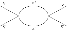
FIG. 4.: Polarization tensor in Fermi theory with an external neutrino current containing an electron-positron loop

The total rate follows from the differential rate by convolution with the neutrino distributions:

$$R_{\nu\bar{\nu}}= \int\frac{d^{3}q_{1}}{(2\pi)^{3}}\int\frac{d^{3}q_{2}}{(2\pi)^{3}}[f_{\nu}(q_{1})f_{\bar{\nu}}(q_{2})$$ (13)

$$-(1-f_{\nu}(q_{1}))(1-f_{\bar{\nu}}(q_{2}))]\>e^{-E/T_{e}}]\>\frac{dR_{\nu\bar{\nu}}}{d^{3}q_{1}d^{3}q_{2}}.$$

Similar expressions for the differential and total rate can be derived for $\nu e^{\pm}$-scattering.

Alternatively the rates can be calculated from the scattering amplitude,

$$\frac{dR_{\nu\bar{\nu}}}{d^{3}q_{1}d^{3}q_{2}}=\frac{1}{2q_{1}2q_{2}}\int\frac{d^{3}p_{1}}{2E_{1}(2\pi)^{3}}[1-n_{e^{+}}(E_{1})]\int\frac{d^{3}p_{2}}{2E_{2}(2\pi)^{3}}$$ (14)

$$[1-n_{e^{-}}(E_{2})]\>(2\pi)^{4}\delta^{4}(Q_{1}+Q_{2}-P_{1}-P_{2})\sum_{i}\langle|{\cal M}|^{2}\rangle,$$ (15)

where $n_{e^{\pm}}(E)=1/[\exp(E\pm\mu)/T+1]$ is the Fermi distribution of the electrons and positrons in the plasma.

FIG. 5.: Ratio of the differential rate in a magnetic field to zero magnetic field for annihilation (solid line) and gyromagnetic absorption (dashed line) of a 4 MeV $\nu$ and a 5 MeV $\bar{\nu}$ in an $e^{\pm}$-plasma at $T=2$ MeV as a function of $B$

FIG. 6.: Annihilation and gyromagnetic absorption rate in an $e^{\pm}$-plasma at $T=2$ MeV as a function of the $\nu$ energy at $B=4\times 10^{15}$ G

FIG. 7.: Annihilation and gyromagnetic absorption rate in an $e^{\pm}$-plasma at $T=2$ MeV as a function of $\theta$, the poloidal angle between the incoming $\bar{\nu}$ and the magnetic field

In addition to medium effects at finite temperature and density we consider a strong magnetic field, which plays an important role in Supernovae and neutron stars. Recently magnetic field strengths above $10^{15}$ G have been observed in so-called magnetars [10]. In a magnetic field the electrons and positrons are in Landau levels, which leads to a modified electron propagator in the polarization tensor. The magnetic field can absorb momentum, allowing for new processes such as the gyromagnetic absorption $\nu\bar{\nu}e^{\pm}\leftrightarrow e^{\pm}$. The advantage of starting from the polarization tensor instead of the scattering amplitude is the automatic inclusion of all possible processes (annihilation, scattering, gyromagnetic absorption).

Using the approach described above, we found a strong modification of the rates of the various processes in fields at $B>10^{15}$ G. In particular there are pronounced peaks in the rates coming from the Landau levels, new processes like the gyromagnetic absorption become important, and the processes show a strong anisotropy, which could play a role in gamma-ray bursts [11]. In the Figures 5 to 7 these features are illustrated.

IV Strange Quark Matter

Quark matter consisting of up, down and strange quarks may exist in the interior of neutron stars or even in form of strangelets, if quark matter is stable, i.e., if it has a higher binding energy than iron [22]. Strangelets have also been discussed as a possible dark matter candidate [14]. So far calculations of the equation of state (EoS) of strange matter are based on an ideal Fermi gas, where sometimes also one-gluon exchange effects are included [9].

Here we want to consider medium effects at finite density and vanishing temperature, which lead to effective quark masses. Using the one-loop quark self energy in the high-density limit, an effectice in-medium quark propagator is constructed. The dispersion relation at zero momentum following from this propagator defines the effective, density dependent quark mass [17]

$$\omega(p=0)=m_{q}^{*}=\frac{m_{q}}{2}+\left(\frac{m_{q}^{2}}{4}+\frac{g^{2}\mu^{2}}{6\pi^{2}}\right)^{1/2},$$ (16)

where $\mu$ is the quark chemical potential of the order of 300 MeV. The coupling constant $g$, typically of the order 2 - 4, can be regarded as a parameter describing the medium effect of the effective quark mass, which arises naturally due to the interactions as known from mean-field theories in many-particle physics. Consequently we replace the ideal Fermi gas by a quasiparticle gas, where e.g. the particle density is now given by

$$\rho(\mu)=\frac{d}{6\pi^{2}}\>[\mu^{2}-{m_{q}^{*}}^{2}(\mu)]^{3/2},$$ (17)

where $d$ is the degree of freedom, e.g. $d=6$ for strange quarks. Similar expressions for the energy density and the pressure determining the EoS can be found.

The introduction of an effective quark mass, typically of the order of 100 MeV, reduces the binding energy of strange quark matter and renders the existence of stable strangelets as a dark matter candidate unlikely [17]. Furthermore we studied the influence of the quark medium effects on strange stars and hybrid stars, i.e. neutron stars containing a quark matter core, by solving the Tolman-Oppenheimer-Volkoff equation using the EoS for quark matter derived above. As shown in Figure 8 the effective quark mass has a negligible effect on the mass-radius relation of strange stars. On the other hand, the presence of a quark matter core, reduces the radius of a neutron star by typically 20 - 30 %, which might have observable consequences [18, 19]. This reduction is caused by a softening of the EoS due to the presence of a mixed phase. It also reduces the maximum mass of the star to about 1.5 $M_{\odot}$.

Recently it has been speculated that quark matter at high density should be in a color superconducting phase [2]. While this could have some consequences for the cooling behavior of neutron stars [3], it probably does not affect bulk properties, such as the mass-radius relation, since the pairing takes place only close to the Fermi surface.

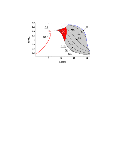
FIG. 8.: Mass-radius relation of pure strange stars (left) and hybrid stars (right) for different values of $g$. QC=star has a quark core, MC=star has a mixed core, H=pure hadron star

V Interaction of Light with the Cosmic Microwave Background

Although the cross section for photon-photon interaction is very small, light propagating through the Universe interacts continuously with the Cosmic Microwave Background (CMB). As discussed in section II photons may acquire an effective mass in a thermal medium. On the other hand, there are very small upper limits for the photon mass deduced from laboratory experiments ($m_{\gamma}<2\times 10^{-16}$ eV) and from the galactic magnetic field ($m_{\gamma}<10^{-27}$ eV) [7]. Therefore it is of interest to consider medium effects of light in the CMB.

The photon-photon interaction of low energy photons ($E\ll m_{e}$) can be described by an effective Lagrangian [12]

$${\cal L}_{I}=-\frac{5\alpha^{2}}{180m_{e}^{4}}\>(F_{\mu\nu}F^{\mu\nu})^{2}+\frac{7\alpha^{2}}{90m_{e}^{4}}\>F_{\mu\nu}F^{\nu\rho}F_{\rho\sigma}F^{\sigma\mu},$$ (18)

where $m_{e}$ is the electron mass, $\alpha$ the fine structure constant, and $F_{\mu\nu}$ the field strength tensor. The lowest order photon self energy following from this Lagrangian is shown in Figure 9.

FIG. 9.: Lowest order photon self energy of the effective theory for photon-photon interaction. The blob denotes the effective 4-photon vertex.

At finite temperature the longitudinal and transverse photon self energy according to Figure 9 is given by [21].

$$\Pi_{L}(p_{0},p) = -\gamma\>p^{2},$$ (19)

$$\Pi_{T}(p_{0},p) = -\gamma\>(p_{0}^{2}+p^{2}),$$ (20)

where $\gamma=(44\pi^{2}/2025)\>\alpha^{2}\>(T/m_{e})^{4}$.

A gauge invariant definition of the Debye mass of the photon relates it to the photon self energy in the following way [16]: $m_{D}^{2}-\Pi_{L}(p_{0}=0,p^{2}=-m_{D}^{2})=0$. Using (20) one finds that the Debye mass vanishes, $m_{D}=0$. Also the effective photon “mass” or plasma frequency, defined as the zero momentum limit of the dispersion relation, $\omega(p)=(1-\gamma)\>p$, vanishes, $\omega(0)=m_{\gamma}=0$. Hence there is no conflict with the measured upper limits of the photon mass.

The electric permittivity and magnetic permeability are also related to the photon self energy:

$$\epsilon = 1-\frac{\Pi_{L}}{p^{2}}=1+\gamma,$$ (21)

$$\frac{1}{\mu} = 1+\frac{\Pi_{T}-p_{0}^{2}\Pi_{L}/p^{2}}{p^{2}}=1-\gamma.$$ (22)

From these quantities the phase velocity $v_{p}$ and the index of refraction $n$ follow as

$$v_{p}=\frac{1}{n}=\frac{1}{\sqrt{\mu\epsilon}}=1-\gamma.$$ (23)

Since the temperature of the Universe drops with time, the phase velocity increases continuously to its vacuum value. Whereas it was given by $v_{p}=1-5.6\times 10^{-31}$, when radiation and matter decoupled at about $T=3000$ K, it increased today at $T=2.7$ K to $v_{p}=1-4.7\times 10^{-43}$. Although this is probably not a measurable effect, it is amusing to note that the speed of light is not a constant in our Universe.

REFERENCES

- [1] Adams, J. B., M. A. Ruderman, and C. H. Woo: 1963, ‘Neutrino Pair Emission by a Stellar Plasma’. Phys. Rev. 129, 1383–1390.
- [2] Alford, M., K. Rajagopal, and F. Wilczek: 1998, ‘QCD at Finite Baryon Density: Nucleon Droplets and Superconductivity’. Phys. Lett. B 422, 247–256.
- [3] Blaschke D., T. Klähn, and D. N. Voskresensky: 2000, ‘Diquark Condensates and Compact Star Cooling’. Astrophys. J. 533, 406–412.
- [4] Braaten, E. and R. D. Pisarski: 1990, ‘Soft Amplitudes in Hot Gauge Theories: A General Analysis’. Nucl. Phys. B 337, 569–634.
- [5] Braaten, E.: 1991, ‘Emissivity of a Hot Plasma from Photon and Plasmon Decay’. Phys. Rev. Lett. 66, 1655–1658.
- [6] Bödeker, D.: 1998, ‘On the Effective Dynamics of Soft Nonabelian Fields at Finite Temperature’. Phys. Lett. B 426, 351–360.
- [7] Caso, C. et al.: 1998, ‘Review of Particle Physics. Particle Data Group’. Eur. Phys. J. C 3, 1–794.
- [8] Colgate, S. A. and R. H. White: 1966, ‘Neutrino-Driven Winds from Young, Hot Neutron Stars’ Astrophys. J. 309, 141–160.
- [9] Farhi, E. and R.L. Jaffe: 1984, ‘Strange Matter’. Phys. Rev. D 30, 2379–2390.
- [10] Gotthelf, E. V., G. Vasisht, and T. Donani et al.: 1999, ‘On the Spin History of X-Ray Pulsar in KES 73: Further Evidence for an Ultramagnetized Neutron Star’. astro-ph/9906122 .
- [11] Hardy, S. J and M. H. Thoma: 2001, ‘Neutrino-Electron Processes in a Strongly Magnetized Thermal Plasma’. Phys. Rev. D 63, 025014-1–12.
- [12] Heisenberg, W. and H. Euler: 1936, ‘Consequences of Dirac’s Theory of Positrons’. Z. Phys. 98, 714–732.
- [13] Landsman, N. P. and C. G. van Weert: 1987, ‘Real and Imaginary Time Field Theory at Finite Temperature and Density’. Phys. Rep. 145, 141–249.
- [14] Madsen, J. and P. Haensel (eds): 1991, ‘Strange Quark Matter in Physics and Astrophysics’. Nucl. Phys. B (Proc. Suppl.) 24B, 1–290.
- [15] Nötzold, D. and G. Raffelt: 1988, ‘Neutrino Dispersion at Finite Temperature and Density’. Nucl. Phys. B307, 924–936.
- [16] Rebhan, A. K.: 1993, ‘Non-Abelian Debye Mass at next-to-leading order’. Phys. Rev. D 48, R3967–R3970.
- [17] Schertler, K., C. Greiner, and M. H. Thoma: 1997, ‘Medium Effects in Strange Quark Matter and Strange Stars’. Nucl. Phys. A 616, 659–679.
- [18] Schertler, K., C. Greiner, P. K. Sahu, and M. H. Thoma: 1998, ‘The Influence of Medium Effects on the Gross Structure of Hybrid Stars’. Nucl. Phys. A 637, 451–465.
- [19] Schertler, K., C. Greiner, J. Schaffner-Bielich, and M. H. Thoma: 2000, ‘Quark Phases in Neutron Stars and a “Third Family” of Compact Stars as a Signature for Phase Transitions’. Nucl. Phys. A 677, 463–490.
- [20] Thoma, M. H.: 2000, ‘New Developments and Applications of Thermal Field Theory’. hep-ph/0010164.
- [21] Thoma, M. H.: 2000a, ‘Photon-Photon Interaction in a Photon Gas’. Europhys. Lett. 52, 498–503.
- [22] Witten, E.: 1984, ‘Cosmic Separation of Phases’. Phys. Rev. D 30, 272–285.