Time-Evolution of the Power Spectrum
of the Black Hole X-ray Nova XTE J1550-564

Abstract

We have studied the time evolution of the power spectrum of XTE J1550-564, using X-ray luminosity time series data obtained by the Rossi X-Ray Timing Explorer satellite. A number of important practical fundamental issues arise in the analysis of these data, including dealing with time-tagged event data, removal of noise from a highly non stationary signal, and comparison of different time-frequency distributions. We present two new methods to understand the time frequency variations, and compare them to the dynamic power spectrum of Homan et al. [2] All of the approaches provide evidence that the QPO frequency varies in a systematic way during the time evolution of the signal.

1 Introduction

Recent years have seen dramatic developments in our ability to study various parts of the universe in wavelength regions inaccessible from the surface of the Earth and using new methods of data acquisition, primarily from NASA satellites. Among the most fascinating are X ray data that are suspected to be emanating from black holes. The X-ray luminosities of such sources are typically highly variable in a quasi-random way, and most investigators take the power spectrum of the time series data as the diagnostic tool of choice. In a number of cases the spectra show peaks at well defined frequencies, but with relatively broad profiles – in contrast to the very narrow peaks of say pulsars, which are strictly periodic. These broad power spectral features indicate a roughly periodic behavior, called quasi periodic oscillations, or QPO’s. A number of investigators have reported time variations in these power spectra.

Variations in the spectra are of course of immense interest because they indicate possible changing physical conditions and hence give basic information about the presumed accretion process – the flow of matter from a disk of gas surrounding the black hole into its deep gravitational potential well. The basic presumption is that the variations are connected with irregularities of the flow, which is presumably turbulent. Progress in this field is crucially dependent on proving that the power spectra are indeed evolving, and studying the properties of such variation.

This paper reports on new tools for studying such spectral evolution, applies them to data on a well known black hole candidate, namely XTE J1550-564, discovered and studied using NASA’s RXTE Satellite. The next section briefly describes the standard tool used by astronomers, with which our methods are to be compared.

2 Dynamic Power Spectra

Astronomers usually approach the question of whether the harmonic and other frequency content of time series are changing over time by computing dynamic power spectra (sometimes called spectrograms) from the time series data. The point of view is that once a spectral feature has been detected and studied by means of ordinary power spectrum analysis [6], then time-frequency analysis [1] is warranted, and the dynamic power spectrum is the tool of choice.

We surveyed the Astronomical Journal and found 15 papers using dynamic power spectra. In all but two cases the method of computation is essentially not stated, but we presume that the authors have computed the ordinary power spectrum in a sliding time-window. This cavalier attitude – as though the method is so obvious and universal as to be barely worthy of mention – implies that astronomers are largely unaware of the shortcomings inherent in the dynamic power spectrum [1].

We have developed two methods that we feel are improvements over the usual tools used by astronomers, but are nevertheless suited to the data modes in use in astronomy.

To exercise our methods we have obtained the raw data used in generating the “Dynamic Power Spectrum” in Figure 19 of [2]. This image shows a QPO initially located around 10 Hz, apparently followed by a transition to lower frequencies, about 5-6 Hz. The picture is particularly interesting because it suggests the existence of a time-varying frequency with a non trivial behavior.

We have been able to duplicate this figure. Since the original data are photon arrival times, one has first to estimate the underlying light intensity (rate of photon arrival). This was apparently done by binning the data – i.e. by dividing the time axis in fixed intervals of constant length $T_{s}$ and counting the photons present in each. We deduce that $T_{s}$ was $\frac{1}{80}$ seconds, and that the instantaneous spectrum was estimated with a Welch’s periodogram. Figure 1 shows our reconstructed dynamic power spectrum, which is essentially identical to that in [2].

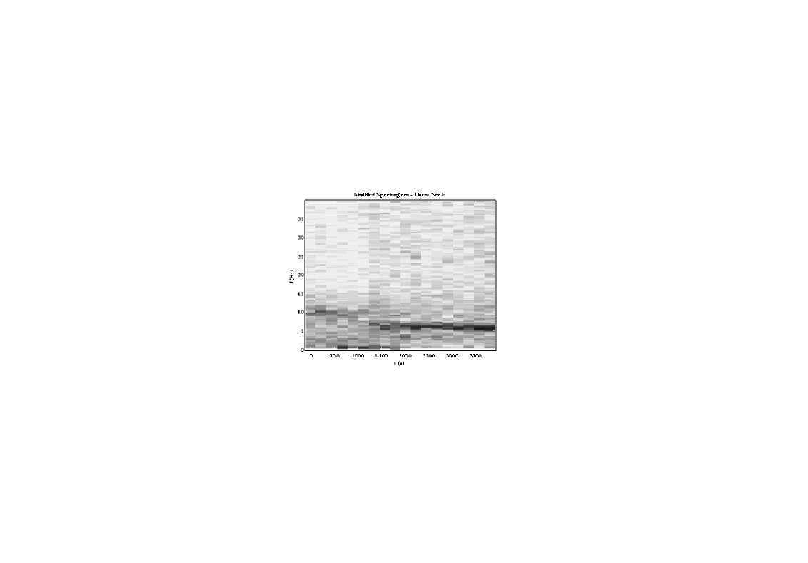
Figure 1: Reconstruction of the “Dynamic Power Spectrum” presented as Fig. 19 in [2]. The presence of a frequency component that makes a transition between 10 Hz to 5-6 Hz is clearly visible.

3 A Time-Frequency Investigation of the X-ray Data

Although binning is an intuitive and universally accepted density estimation procedure, many other methods have more appealing properties [5], especially considering that some additional signal processing has to be done on the estimated density. A famous approach is the kernel method that consists in averaging the number of events (photons) contained in a relatively narrow window that moves continuously along the data. The average is weighted with a normalized kernel that is more or less concentrated about the center of the window. Typical kernels are hence Gaussian, Hanning, triangular, etc. The advantages in applying the kernel methods are several:

• no dependence on phasing of the bins relative to the signal (the dependence on bin size is replaced with that on the width of the kernel)

• the resulting density inherits properties of the window (e.g. it can be differentiated to the same order as the window itself)

• noise (and quantization) are suppressed

We therefore decided to apply the kernel method, using a normalized Hanning window.

Inspection of either density estimate indicates the presence of slowly varying components, on time scales $\geq 0.3$ second (corresponding to frequencies below 3 Hz). To suppress this feature, with the objective to highlight the presence of the QPO, we applied a high-pass filter to the data, using the forward-backward technique with a simple elliptic filter. This method eliminates the nonlinear phase distortion introduced by the filter that can produce undesired effects in the time-frequency plane.

At this point, because of the high noise level (due almost entirely to Poisson counting fluctuations), we estimate the instantaneous spectrum by applying the so called “sliding estimator” [7] to the density. This estimator is the natural extension to the spectrogram [1], and is computed by evaluating Welch’s periodogram of a windowed version of the signal. The window is slid continuously along the signal, and hence the dynamic power spectrum can be seen as a subcase of this method. Fig. 2 represents the Time-Frequency plane obtained with this technique. (The more expressive color image can be found on the CD rom of the proceedings or at the web page helinet.polito.it/sasgroup/ sliding.htm). The joint use of kernel method, highpass filtering, and sliding estimator confirms the presence of a time-varying spectrum in an outstanding way.

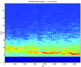
Figure 2: Time-frequency plot of the light intensity emanating from the black hole obtained using the sliding estimator technique.

In particular it is possible to notice the first concentration of the QPO around 10 Hz and then the transition to a central frequency around 6 Hz. A more careful observation points out two interesting facts:

1. the transition is a “complex” event, because it seems to involve a frequency bifurcation around $t=800$ seconds;

2. the QPO, especially after the transition for $t>1200$ s is well represented by what is called a one component signal – that is, a time-varying frequency with slowly varying amplitude. This can also be noticed in the first part of the QPO, but with a smaller intensity.

It is also useful to observe how the noise is reduced, especially at higher frequencies, by the application of the kernel method, and how the QPO is highlighted by the highpass filtering.

4 A Further Development in the Analysis of the X-ray Data

In the first part of this paper we have presented a nonparametric estimation of the instantaneous spectrum of the intensity of light. This analysis has pointed out that the QPO seems to be made by a time-varying frequency that also shows a transition from the 10-11 Hz band to the 5-6 Hz band. To accomplish this analysis, we adopted on purpose a nonparametric approach. That is, we did not make use of any model for the data, because still we were not sure of the possible presence of oscillations in the signal.

Now that the result obtained by using the sliding estimator points out with a good probability the existence of this oscillation, we intend to highlight it by doing a further signal processing on the estimated time-frequency distribution. In doing so we adopt a semi-parametric approach, using both additional nonparametric methods and also a parametric model for the background noise that will help us extracting the useful information.

For convenience we call $P(t,\omega)$ the estimated instantaneous spectrum obtained in the previous section, that we set as the starting point of the new analysis. This analysis is based on three main steps: noise whitening, thresholding and amplitude normalization of the QPO. A description of the steps follows, in which we indicate with $P_{k}(t,\omega)$ the time-frequency distribution obtained at the $k$-th step applying the proposed signal processing.

4.1 Noise Whitening

One of the characteristics of the QPO that we have highlighted with the sliding estimator technique, is that it is embedded in a high level non-white noise, as can be confirmed by visual inspection of Fig. 2. This noise does not have a flat spectrum, and our aim here is to whiten it, that is to force it to have a flat behavior.

Of course we know that in what we call noise, that is the spectral region outside the QPO, there might be other important features of the black hole candidate (for example other low energy QPOs), but as said before here we want to focus our attention on the main QPO. We accomplish the whitening in three steps.

• We first estimate the power spectral density $|N(\omega)|^{2}$ of the noise by integrating with respect to time the time-frequency distribution $P(t,\omega)$,

  $$|N(\omega)|^{2}=\int P(t,\omega)dt$$ (1)

  This quantity is called frequency marginal in time-frequency analysis, and can be seen as an approximation of the power spectrum of the signal.

• Then we fit the obtained noise density $|N(\omega)|^{2}$ with a cubic polynomial to obtain a fitted spectrum $|N_{f}(\omega)|^{2}$, paying attention to force the fitted curve to be grater or equal to a small positive parameter $\delta$. We point out that the noise density $|N(\omega)|^{2}$ is estimated outside the QPO region, whereas the fitted density $|N_{f}(\omega)|^{2}$ is valid throughout the entire band.

• Finally we whiten the time-frequency distribution $P(t,\omega)$ by dividing it by the estimated noise

  $$P_{1}(t,\omega)=\frac{P(t,\omega)}{|N_{f}(\omega)|^{2}}$$ (2)

4.2 Thresholding

Now that we have whitened the noise, and we expect it to show a flatter spectrum, we threshold the obtained distribution $P_{1}(t,\omega)$ to extract the QPO. To do this we act in two steps

• We estimate a threshold $\theta$ by inspecting the frequency marginal of $P_{1}(t,\omega)$.

• We then subtract the threshold from the time-frequency distribution, setting to zero any negative value the resulting difference may have

  $$P_{2}(t,\omega)=P_{1}(t,\omega)-\theta,\quad P_{2}(t,\omega)\geq 0$$ (3)

4.3 Amplitude Normalization of the QPO

As a final step we want to compensate the instantaneous amplitude variations of the QPO that can be noticed from Fig. 2, and that are probably responsible of the changing in time of the energy concentration along the QPO instantaneous frequency. To do this we normalize the instantaneous spectrum at each time by diving it by its estimated energy at that time, that is

$$P_{3}(t,\omega)=\frac{P_{2}(t,\omega)}{\int P_{2}(t,\omega)d\omega}$$ (4)

where the integral of $P_{2}$ over time is used as an approximation to the energy of the instantaneous signal at that time (time marginal).

In Fig. 3 we plot the final instantaneous spectrum $P_{3}(t,\omega)$, where it is possible to notice the effects of the above procedure. The analysis done so far better highlights what seems to be the time-varying behavior of the QPO central frequency. Our analysis to date seems to elucidate QPO variations better than conventional dynamic power spectra, but further studies are needed, mainly of the algorithm’s reliability and immunity to artifacts.

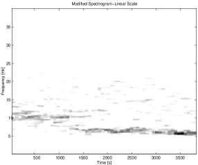
Figure 3: Extraction of the QPO with a more advanced and quasi-parametric signal processing.

Acknowledgment: Work supported by the NSA HBCU/MI program and the NASA Applied Information Systems Research Program.

References

- [1] L. Cohen, Time-Frequency Analysis, Prentice-Hall, 1995.
- [2] J. Homan, R. Wijnands, M. van der Klis, T. Belloni, J. van Paradijs, M. Klein-Wolt, R. Fender and M. Mendez, “Correlated X-Ray spectral and Timing Behavior of the Black Hole Candidate XTE J1550-564” Astrophysical Journal Supplement Series, Vol. 132, pp. 377-402, 2001.
- [3] D. Nelson,“Special Purpose Correlation Functions for Improved Signal Detection and Parameter Estimation,” in Proceedings of IEEE Conference on Acoustics, Speech and Signal Processing, pp.73-76, April, 1993.
- [4] J. Scargle, et. al. “The Quasi-Periodic Oscillations and Very-Low Frequency Noise of ScorpioX-1 as Transient Chaos: A Dripping Handrail?”, Ap. J. Lett., 411, pp. L91-L94.
- [5] B. W. Silverman Density Estimation for Statistics and Data Analysis Chap and Hall/CRC Press, Inc., 1986.
- [6] M. van der Klis, “Fourier Techniques in X-Ray Timing,” in Proc. NATO Advanced Study Institute, Timing Neutron Stars, 1988.
- [7] M. Bayram and R. G. Baraniuk, “Multiple window time frequency analysis,” in Proceedings of the IEEE SP International Symposium on Time Frequency and Time Scale Analysis, pp. 173–176, (Paris, France), June 1996; F. Cakrak and P. Loughlin, “Multiple window non–linear time–varying spectral analysis,” IEEE Transactions on Signal Processing, to appear, 2000; J. Pitton, “Time frequency spectrum estimation: an adaptive multitaper method,” in IEEE Int. Sym. Time Frequency and Time Scale Analysis, pp. 665–668, (Pittsburgh, PA), 1998; G. Frazer and B. Boashash, “Multiple window spectrogram and time frequency distributions,” in Proc. IEEE Int. Conf. Acoust., Speech, Signal Processing, ICASSP ’94, vol. IV, pp. 293–296, 1994.