Cosmic Microwave Background anisotropies with mixed isocurvature perturbations

Abstract

Recently high quality data of the cosmic microwave background anisotropies have been published. In this work we study to which extent the cosmological parameters determined by using this data depend on assumptions about the initial conditions. We show that for generic initial conditions, not only the best fit values are very different but, and this is our main result, the allowed parameter range enlarges dramatically.

]

I Introduction

The discovery of anisotropies in the cosmic microwave background (CMB) by the COBE satellite in 1992 [1] has stimulated an enormous activity in this field which has culminated recently with the high precision data of the BOOMERanG [2], DASI [3] and MAXIMA-1 [4] experiments. The CMB is developing into the most important observational tool to study the early Universe. So far, this data have however mainly been used to determine cosmological parameters for a fixed model of initial fluctuations, namely scale invariant adiabatic perturbations [5, 6, 7, 8, 9, 10, 11, 12].

In this work we investigate to which extent the determination of cosmological parameters depends on initial conditions. Rather than exploring the most general parameter space, we mainly want to show in a specific example how the allowed parameter range is enlarged when the requirement for purely adiabatic initial conditions is loosened. Therefore, in order to limit the computational effort we have chosen to vary some cosmological parameters and keep the others fixed. We have set the total density parameter $\Omega_{\rm tot}=\Omega_{\Lambda}+\Omega_{\rm m}=1$ and fixed $\Omega_{\Lambda}=0.7$ and $\Omega_{\rm m}=\Omega_{\rm c}+\Omega_{\rm b}=0.3$. Here $\Omega_{\Lambda}$ denotes the density parameter due to a cosmological constant, $\Omega_{\Lambda}=\Lambda/3H_{0}^{2}$, while $\Omega_{\rm c}$ and $\Omega_{\rm b}$ are the density parameters of cold dark matter (CDM) and baryons respectively, and $H_{0}=100h{\;\mathrm{km}}{\;\mathrm{s}^{-1}}{\;\mathrm{Mpc}^{-1}}$ is the Hubble parameter today. For fixed $\Omega_{\Lambda}$, $\Omega_{\rm c}$ and spectral index $n_{\rm S}=1$ we determine the parameters $h$ and $\omega_{\rm b}\equiv\Omega_{\rm b}h^{2}$ for generic initial conditions.

II Initial conditions

A study considering the adiabatic together with just one isocurvature mode has been undertaken recently [13]. To choose an even more generic set of initial conditions we follow the procedure outlined in Ref. [14]. The matter components present in the “standard” universe are CDM, baryons, massless neutrinos ($\nu$) and photons (${\rm\gamma}$). Usually adiabatic initial conditions are assumed for the perturbations of these components. In Newtonian or flat-slicing gauge, this implies

$\displaystyle\Delta_{\rm c}=\Delta_{\rm b}=\frac{4}{3}\Delta_{\rm\gamma}=\frac{4}{3}\Delta_{\rm\nu},\mbox{ and }V_{\rm c}=V_{\rm b}=V_{\rm\gamma}=V_{\rm\nu},$where $\Delta_{i}$ and $V_{i}$ are the density fluctuation and the peculiar velocity potential of component $i$. However, this does not represent the most general set of possible initial conditions for cosmological perturbations. Apart from the adiabatic mode given above there are a baryon isocurvature mode (${\rm BI}$) a CDM isocurvature mode (${\rm CI}$) a neutrino isocurvature density mode (${\rm NID}$) and a neutrino isocurvature velocity mode (${\rm NIV}$). The precise definition of these modes is given in Ref. [14] and some observable consequences of deviations from a pure adiabatic model were already investigated in Ref. [15]. The most generic initial conditions are then given by a positive definite $5\times 5$ matrix $M$ representing the amplitude of each of these modes, including all the possible cross-correlations (see Ref. [14]; a gauge-invariant formulation of the initial conditions is given in Ref. [16]). We have noticed that implementing the initial conditions for all the modes in synchronous gauge was somewhat tricky, while this procedure is very simple and numerically unproblematic in gauge-invariant formalism.

For a fixed set of cosmological parameters we first compute the CMB anisotropy spectrum $C^{ij}_{\ell}$ when only one of the elements of the correlation matrix is non-zero ($M_{ij}=1$, all other elements vanish) with a fixed spectral index $n_{\rm S}=1$ for all modes. Next we set

$$C_{\ell}(M)=\sum_{i,j=1}^{5}M_{ij}C^{ij}_{\ell}~{}.$$ (1)

As already noticed in Ref. [17], the ${\rm BI}$ and ${\rm CI}$ components of the correlation matrix are identical, up to an irrelevant multiplicative constant (which is due to the fact that $\Omega_{\rm b}\neq\Omega_{\rm c}$). We have therefore restricted our analysis to the four modes ${\rm AD}$, ${\rm CI}$, ${\rm NID}$, ${\rm NIV}$ without loss of generality. We then vary the correlation matrix $M$ and the cosmological parameters $\omega_{\rm b}$ and $h$ to search for the best fit to the data using a maximum likelihood method.

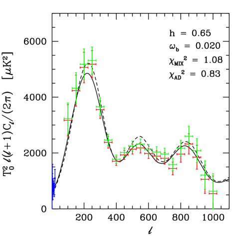
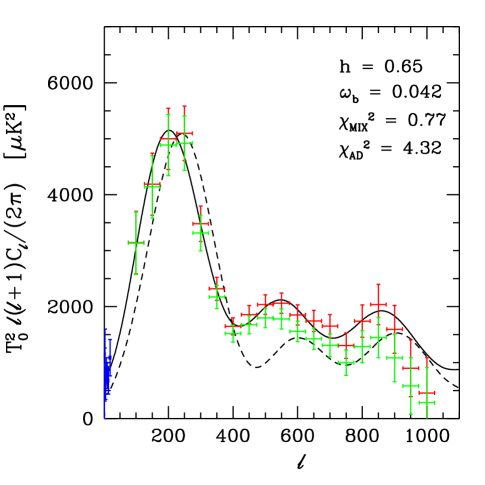
FIG. 1.: CMB anisotropy spectrum for different values of the cosmological parameters $\omega_{\rm b}$ and $h$. We have shown the best-fit corresponding to a purely adiabatic case (dashed line) and allowing the most general set of initial conditions (solid line). The calibration and the beam size of the BOOMERanG data have been optimized to fit the mixed model (red/dark error bars) or the adiabatic model (green/light error bars). The parameter choice on top ($\omega_{\rm b}=0.02$, $h=0.65$) can be fitted by both models while the values $\omega_{\rm b}=0.042$, $h=0.65$, can only be fitted by a mixed model.

Since the main point of this paper is to clarify the role of initial conditions and not to obtain the most realistic set of cosmological parameters, we restrict our analysis to the COBE[1] and BOOMERanG [2] data. For the BOOMERanG data we also take into account the calibration and the beam size uncertainties [2] which we treat just like two additional (normally distributed) parameters of the problem. The best fits are computed using a downhill simplex method [18] initiated after choosing a starting point randomly. Although this is certainly not the best method it proved to be sufficient for our purpose. In practice, each fit is the best fit among 15,000 minimization runs with random initial conditions. The positive semi-definiteness of the correlation matrix $M$ is insured by penalty functions on the sub-determinants of $M$ (more details are given in [16]). It turns out that the topology of the $\chi^{2}$ surface on our $14$-dimensional parameter space is quite complicated with many local minima and probably many degeneracies (see also the example discussed in [13]).

In Fig. 1 we show the best fit spectra for two different choices of the cosmological parameters $\omega_{\rm b}$ and $h$. Both of them are good fits if we allow for mixed initial conditions. On the plot we have also indicated the reduced $\chi^{2}$. For a fixed choice of the parameters $\omega_{\rm b}$, $h$ the purely adiabatic model has only $3$ parameters (the amplitude of the adiabatic mode, the BOOMERanG calibration and beam size). With 26 data points (7 from COBE and 19 from BOOMERanG) this leads to $F_{\rm AD}=26-3=23$ degrees of freedom, while the mixed models have a symmetric $4\times 4$ matrix determining the initial amplitude, leading to a total of $12$ parameters and hence only $F_{\rm MIX}=14$ degrees of freedom. If we also vary $\omega_{\rm b}$ and $h$, the number of degrees of freedom is lowered by $2$. It is of course not surprising that for the parameters $h=0.65$, $\omega_{\rm b}=0.02$, which are well fitted by the adiabatic model, the reduced $\chi^{2}$ of the adiabatic model is somewhat lower than the one of the mixed model. For the mixed model, the absolute $\chi^{2}$ is always lower than the one of the adiabatic model since the latter one is contained in the generic class of mixed models, but the reduced $\chi^{2}$ can of course be higher since it is divided by a smaller number of degrees of freedom, $F_{\rm MIX}<F_{\rm AD}$. This is actually the case for the parameters choice in the top panel of Fig. 1.

To indicate what happens when models with mixed initial conditions are admitted we determine the likelihood functions of the cosmological parameters $\omega_{\rm b}$ and $h$ by marginalizing over the initial conditions and the BOOMERanG calibration and beam size. The result is shown in Fig. 2 where the likelihood contours in the $(\omega_{\rm b},h)$ plane for likelihoods of 50%, 68%, 95%, 99% are indicated for mixed models (top) and for purely adiabatic models (bottom). This figure is our main result. It is quite amazing to see to which extent the innermost good fit contour opens up once we allow for isocurvature components. Strangely, the only excluded region which remains is the upper left corner corresponding to the value of $\omega_{\rm b}$ inferred from big bang nucleosynthesis [19] and the Hubble space telescope key project value for the Hubble parameter [20] of $h=0.72\pm 0.08$.

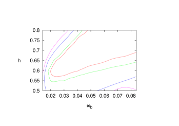
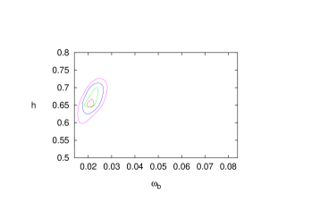
FIG. 2.: The likelihood contours of 50%, 68%, 95%, 99% are indicated in the $(\omega_{\rm b},h)$ plane for mixed models (top) and for purely adiabatic models (bottom). The likelihoods are obtained by marginalization over the BOOMERanG calibration and beam size as well as over the initial conditions given by the matrix $M$ for mixed models and by the amplitude of the adiabatic mode for adiabatic models. For the mixed model, the lowest $\chi^{2}$ corresponds to even higher values of $\omega_{\rm b}$ and $h$ than those shown in the plot.

There is absolutely no upper limit for $\omega_{\rm b}$ within the regime investigated here! Actually, this can be understood by noting that with adiabatic initial conditions, the strongest feature of a high baryon density universe is the asymmetry between even and odd acoustic peaks, but recalling that this asymmetry exists only in the matter dominated era and not in the radiation dominated era. With the parameters we have chosen here, the high value of $\Omega_{\Lambda}$ implies a low matter content and hence, equivalence between radiation and matter happens not long before decoupling. For high values of $h$, the equivalence occurs earlier and the asymmetry of the peaks allows to put upper limits on the baryon density in purely adiabatic models. The second feature of high baryon density is to reduce the sound horizon and therefore to shift the acoustic peaks to the right. These two effects constrain the baryon density most strongly in the class of purely adiabatic models. In the case of mixed initial conditions, it is known that the presence of the isocurvature modes, especially the neutrino isocurvature modes, can not only shift the peaks significantly but also change their relative heights [17] (see lower panel of Fig. 1). A high baryon density can therefore easily be accommodated in this framework. Note however that for high $\omega_{\rm b}$ and low $h$, it is difficult to find a good fit, even for mixed models, because there is not enough power in the secondary peak region. The reason is that the early integrated Sachs-Wolfe effect boosts the first peak.

We define the isocurvature content of a mixed model by $\alpha=(M_{22}+M_{33}+M_{44})/\mbox{trace}M$, where $M_{11}$ denotes the adiabatic mode amplitude. The isocurvature content in the good fit model shown in the top panel of Fig. 1 is only $\alpha=0.12$, while for the parameter choice in the bottom panel $\alpha=0.69$. Hence, if the cosmological parameters are close to those chosen in the top panel, we can conclude that the cosmic perturbations are predominantly adiabatic. In Fig. 3 we show the isocurvature content $\alpha$ of the best fit model obtained by minimizing $\chi^{2}$ by variation of the initial conditions at fixed values of the cosmological parameters. Clearly, the further we move away from the parameter region well fitted by the purely adiabatic model, the higher becomes the isocurvature contribution needed to fit the data.

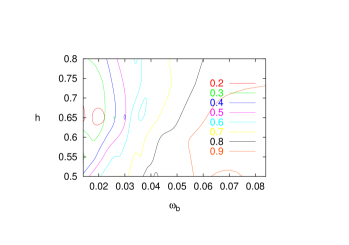
FIG. 3.: The isocurvature content $\alpha$ of the best fit mixed model at fixed parameter values $(\omega_{\rm b},h)$ is indicated. The contours $\alpha=0.2$ to $0.9$ in steps of $0.1$ are shown.

The main non-adiabatic component of our best fits is the ${\rm NID}$ mode. This was to be expected as this mode and its correlator with the adiabatic mode can shift the peak positions and can substantially add or subtract from the second peak. It is known that for interacting species the non adiabatic part of the perturbations tends to decay with time. Therefore the generation of this ${\rm NID}$ component can only occur after neutrino decoupling, that is at $T\lesssim 1{\;\mathrm{MeV}}$. Whether or not such a phenomenon can occur at low energy is an open question. However, a neutrino isocurvature perturbation can also be due to a fourth species of sterile neutrinos which may have decoupled very early in the history of the Universe. The same remark applies of course also to the CDM isocurvature mode. Note that the energy density of this fourth neutrino type cannot be very high in order not to contradict the light element abundances, but there is nothing which prevents (at least in principle) the presence of large perturbations in this fluid.

III Conclusion

We have shown that allowing for isocurvature contributions one may very well fit present CMB data with a set of cosmological parameters which differs considerably from the one preferred by adiabatic perturbations. More important, allowing for generic initial conditions, the ranges of cosmological parameters which can fit the CMB anisotropy data widen up to an extent to become nearly meaningless.

On the other hand, assuming measurements of cosmological parameters from other methods like direct measurements of the Hubble parameter which yield $h\sim 0.65$ and big bang nucleosynthesis which implies $\omega_{\rm b}\sim 0.02$, we can use the CMB to limit the isocurvature contribution in the initial conditions (or other unconventional features) and thereby learn something about the very early universe, the inflationary phase which probably has generated these initial conditions.

We believe that it is already interesting to note that for cosmological parameters in the range preferred by other, CMB independent, measurements ($\Omega_{\Lambda}\sim 0.7$, $\Omega_{\rm m}\sim 0.3$, $h\sim 0.65$, $\omega_{\rm b}\sim 0.02$) the isocurvature contribution in the initial conditions has to be relatively modest.

Finally, our work shows the danger of calling parameter estimation by CMB anisotropy experiments a “parameter measurement” since the results depend so sensitively on the underlying model assumptions. We rather consider CMB anisotropies as an excellent tool to test model assumptions or consistency. In the light of these findings, the importance of non-CMB measurements of cosmological parameters can clearly not be overstated. In short, CMB seems to be a better tool to investigate the primordial parameters (i.e., the initial conditions) rather than the cosmological parameters ($\Omega$’s, $h$ etc). Hopefully, measuring the CMB polarization will represent an additional non-trivial mean to remove the degeneracy present between cosmological parameters and initial conditions. This has been studied in detail in Ref. [17]. The main reason for this is that polarization, which is induced only during decoupling, is mostly sensitive to the photon dipole $V_{\rm\gamma}$ rather than the photon density perturbation $\Delta_{\rm\gamma}$, these two quantities depending in a different way on the initial conditions. In the same vein, using the normalization of the matter power spectrum (provided it can be measured accurately…) also helps to break some of the degeneracies induced by the isocurvature modes.

- [1] G.F. Smoot et al., ApJ396, L1 (1992); C.L. Bennett et al., ApJ430, 423 (1994); M. Tegmark and A.J.S. Hamilton, in “18th Texas Symposium on relativistic astrophysics and cosmology”, edited by A.V. Olinto et al., pp 270 (World Scientific, Singapore, 1997).
- [2] C.B. Netterfield et al., preprint astro-ph/0104460 (2001).
- [3] N.W. Halverson et al., preprint astro-ph/0104489 (2001).
- [4] A.T. Lee et al., preprint astro-ph/0104459 (2001).
- [5] A. Balbi, et al., ApJ545, L5 (2000).
- [6] A. Jaffe et al., Phys. Rev. Lett.86, in press (2001).
- [7] M. Tegmark, M. Zaldarriaga, Phys. Rev. Lett.85, 2240 (2000).
- [8] M. Tegmark, M. Zaldarriaga and A. Hamilton, Phys. Rev. D63, 043007 (2001).
- [9] A. Lange et al., Phys. Rev. D63, 042001 (2001).
- [10] C. Pryke et al., preprint astro-ph/0104490 (2001).
- [11] R. Stompor et al., preprint astro-ph/0105062 (2001).
- [12] P. de Bernardis et al., preprint astro-ph/0105296 (2001).
- [13] L. Amendola et al., preprint astro-ph/0107089 (2001).
- [14] M. Bucher, K. Moodley and N. Turok, Phys. Rev. D62, 083508 (2000).
- [15] D. Langlois and A. Riazuelo, Phys. Rev. D62, 043504 (2000).
- [16] R. Trotta, Diploma thesis at ETH Zürich (2001).
- [17] M. Bucher, K. Moodley and N. Turok, Phys. Rev. Dsubmitted, preprint astro-ph/0012141 (2000).
- [18] W.H. Press, S.A. Teukolsky, W.T. Vetterling and B.P. Flannery, Numerical recipes, (Cambridge University Press, Cambridge, England, 1988).
- [19] S. Burles, K.M. Nollet and M.S. Turner, ApJsubmitted, preprint astro-ph/0010171.
- [20] W.L. Freedman et al., ApJ553, 47 (2001) (astro-ph/0012376).