Implication of $\Omega_{m}$ through the Morphological Analysis
of Weak Lensing Fields

Abstract

We apply the morphological descriptions of two-dimensional contour map, the so-called Minkowski functionals (the area fraction, circumference, and Euler characteristics), to the convergence field $\kappa(\mbox{\boldmath$\theta$})$ of the large-scale structure reconstructed from the shear map produced by the ray-tracing simulations. The perturbation theory of structure formation has suggested that the non-Gaussian features on the Minkowski functionals with respect to the threshold in the weakly nonlinear regime are induced by the three skewness parameters of $\kappa$ that are sensitive to the density parameter of matter, $\Omega_{\rm m}$. We show that, in the absence of noise due to the intrinsic ellipticities of source galaxies with which the perturbation theory results can be recovered, the accuracy of $\Omega_{\rm m}$ determination is improved by $\sim 20\%$ using the Minkowski functionals compared to the conventional method of using the direct measure of skewness.

1 Introduction

Weak gravitational lensing caused by the large-scale structure (LSS) of the universe distorts the images of distant galaxies. This phenomenon is the so-called cosmic shear, which offers us the unique opportunity to measure directly the projected power spectrum of dark matter fluctuations regardless of the relation between dynamical states of the dark matter and luminous matter (Blandford et al. (1991); Miralda-Escude (1991); Kaiser (1992)). Recently, several independent measurements of cosmic shear have been made from deep ’blank-field’ CCD imaging surveys, and reported significant detections of shear variance (van Waerbeke et al. (2000); Wittman et al. (2000); Bacon, Refregier & Ellis (2000); Kaiser, Willson & Luppino (2000); Maoli et al. (2000)).

Due to the nonlinear evolution of density fluctuation field in the large-scale structure, the cosmic shear field on small angular scale is expected to display significant non-Gaussian features. Even in this case, for the second moment analysis it has been shown that the numerical results from the ray-tracing simulations are in remarkably good agreements with the theoretical predictions using the fitting formula for the nonlinear matter power spectrum (Jain, Seljak & White (2000); Hamana, Martel & Futamase 2000a ). On the other hand, the higher order statistics can provide additional cosmological information associated with the non-Gaussian features. Especially, the normalized skewness parameter of the convergence field can be a sensitive indicator of the density parameter of matter, $\Omega_{m}$ (Bernardeau, van Waerbeke & Mellier (1997)). However, unfortunately the highly nonlinear evolution of third order statistics cannot be simply described by the fitting formula for the nonlinear power spectrum alone. Recently, the extended method that allows us to perform the skewness calculations in the strongly nonlinear regime has been developed using “hyper-extended perturbation theory” (HEPT) (Hui (1999); Scoccimarro & Frieman (1999)). Nevertheless, several works using the ray-tracing simulations have revealed that the value predicted by HEPT at relevant angular scales does not agree so well with the numerical results of skewness parameter (Jain, Seljak & White (2000); White & Hu (2000); Hamana et al. 2000b ). Moreover, we would like to stress that it is difficult to have a physical meaning for the fitting formula beyond an empirical one. Therefore, it will be worth exploring again a new method to effectively extracting the non-Gaussian features of the convergence field in the weakly nonlinear regime based on the perturbation theory, which relies on a more firm physical basis of the structure formation.

A possible method we propose is to use the Minkowski functionals with respect to level threshold; this is motivated by the fact that the functionals give the complete morphological descriptions of a considered field (Schmalzing & Buchert (1997)). For a two-dimensional case, the Minkowski functionals consist of the area fraction, circumference and Euler characteristics of the isocontour curves, where the Euler characteristics is equivalent to the genus statistics often used in the cosmology (Gott, Melott & Dickinson (1986)). Recently, Matsubara & Jain (2000) applied the genus curve to the convergence field reconstructed from the ray-tracing simulations, and found that the nonlinear evolution of convergence induces a deviation from the specific curve of genus for the Gaussian case. On the other hand, the theoretical predictions based on the perturbation theory have shown that the non-Gaussian features on the Minkowski functionals are completely characterized by the skewness parameters of the convergence field in the weakly nonlinear regime (Matsubara (2000) and see also equation (1)). These results offer a possibility to extract the skewness parameters using the Minkowski functionals of the reconstructed convergence field. The purpose of this Letter is thus to investigate how accurately $\Omega_{\rm m}$ can be determined from the skewness parameters estimated by fitting the numerical results to theoretical predictions of the Minkowski functionals.

2 The Ray-Tracing Simulation and the Minkowski Functionals

We use shear and convergence fields modeled from the ray tracing simulations through the dark matter distribution of N-body simulations following the previous methods by Hamana, Martel & Futamase 2000a and White & Hu (2000). The original N-body simulations of the large-scale structure were performed with the P³M code (see Jing & Fang (1994) and Jing (1998) in detail). The following discussions focus on two cosmological models, summarized in Table 1, and we used three different realizations for each model. As for the power spectrum of matter fluctuations, we assume the cold dark matter (CDM) model with the transfer function given by Bardeen et al. (1986) and the shape parameter $\Gamma=\Omega_{0}h$. All the simulations employ $256^{3}$ ($\approx 17$ million) particles in a ($100h^{-1}$Mpc)³ comoving box and start at redshift $z_{i}=36$. The gravitational softening length $\epsilon$ is $39h^{-1}$kpc.

We use the multiple lens-plane algorithm to follow the propagations of light rays through the simulated matter distributions. In this algorithm, the matter content of each box at a certain redshift is projected onto a single plane perpendicular to the line of sight. We use typically $\sim 20$ equally spaced lens-planes in the comoving distance between source and observer. The particle positions on each plane are interpolated onto a grid of size $2048^{2}$. In order to avoid possible correlations between different lens-planes, in each plane we choose one of the three realizations at the considered redshift and then project the mass distribution along a randomly chosen one of the three coordinate axes, translate the mass distribution by a random vector, and randomly rotate it in a unit of $\pi/2$. We consider a set of lens-planes between the source and observer as a different realization and use ten such realizations to estimate the cosmic variance associated with the measurements of weak lensing fields. Further details of the ray-tracing simulation are given in Hamana, Martel & Futamase (2000).

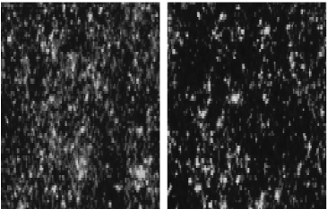
Figure 1: The reconstructed convergence maps used to compute the Minkowski functionals for a field of $3^{\circ}$ on a side. Two cosmological models are shown: SCDM model (left) and $\Lambda$CDM model (right).

The fields we use are $3^{\circ}$ on a side. Each light ray is traced by the Born approximation and hence can be handled as a straight line that radially extends from observer. Throughout this Letter, we assume that all source galaxies are at a redshift of $z_{s}=1$ and that their number densities is $n=30\rm{~{}arcmin}^{-2}$. We then make the cosmic shear field, $\gamma(\mbox{\boldmath$\theta$})$, on each grid from the ray-tracing simulations, and perform the smoothing on $\gamma(\mbox{\boldmath$\theta$})$ by using a top-hat filter. Using the relation between the Fourier transforms $\kappa(\mbox{\boldmath$\theta$})$ and $\gamma(\mbox{\boldmath$\theta$})$, $\hat{\kappa}(\mbox{\boldmath$l$})=[(l_{1}^{2}-l_{2}^{2})\hat{\gamma}_{1}(\mbox{\boldmath$l$})+2l_{1}l_{2}\hat{\gamma}_{2}(\mbox{\boldmath$l$})]/l^{2},$ and assuming the periodic boundary condition, $\kappa(\mbox{\boldmath$\theta$})$ is reconstructed on each grid from the cosmic shear field. Figure 1 shows examples of the reconstructed convergence field. To compute the Minkowski functionals, we label the convergence field by the threshold value $\nu(\mbox{\boldmath$\theta$})$ that is defined by $\nu(\mbox{\boldmath$\theta$})\equiv\kappa(\mbox{\boldmath$\theta$})/\sigma_{0}$, where $\sigma_{0}$ is the rms of $\kappa$ defined by $\sigma^{2}_{0}\equiv\langle{\kappa^{2}}\rangle$.

In a two-dimensional case, the Minkowski functionals are the area fraction $v_{0}(\nu)$, circumference $v_{1}(\nu)$, and Euler characteristics $v_{2}(\nu)$ for the isocontour curve with threshold $\nu$ that fully characterize the morphology of the field. The Euler characteristic is a purely topological quantity, which is equal to the number of isolated high-threshold regions minus the number of isolated low-threshold regions. To calculate the Minkowski functionals for the reconstructed convergence field given as pixel data, we employed the method developed by Winitzki & Kosowsky (1997).

On the other hand, under the hypothesis that the initial perturbations are Gaussian as supported by the inflationary scenario, Matsubara (2000) recently derived the analytical formula of the Minkowski functionals based on the perturbation theory that can be applied to the weakly nonlinear convergence field:

$$v_{0}(\nu) = \frac{1}{2}\mbox{erfc}\left(\frac{\nu}{\sqrt{2}}\right)+\frac{1}{6\sqrt{2\pi}}\mbox{e}^{-\nu^{2}/2}\sigma_{0}s_{0}\mbox{H}_{2}(\nu),$$

$$v_{1}(\nu) = \frac{1}{8\sqrt{2}}\frac{\sigma_{1}}{\sigma_{0}}\mbox{e}^{-\nu^{2}/2}\left\{1+\sigma_{0}\left(\frac{s_{0}\mbox{H}_{3}(\nu)}{6}+\frac{s_{1}\mbox{H}_{1}(\nu)}{3}\right)\right\},$$

$$v_{2}(\nu) = \frac{1}{2(2\pi)^{\frac{3}{2}}}\frac{\sigma_{1}^{2}}{\sigma_{0}^{2}}\mbox{e}^{-\nu^{2}/2}\left\{\mbox{H}_{1}(\nu)+\sigma_{0}\left(\frac{s_{0}\mbox{H}_{4}(\nu)}{6}+\frac{2s_{1}\mbox{H}_{2}(\nu)}{3}+\frac{s_{2}}{3}\right)\right\},$$ (1)

where $\sigma_{1}$ is defined by $\sigma^{2}_{1}\equiv\langle{(\nabla\kappa)^{2}}\rangle$ and H${}_{n}(\nu)$ is the $n$th order Hermite polynomial. $s_{0}$, $s_{1}$, and $s_{2}$ denote the skewness parameters defined by $s_{0}\equiv\langle{\kappa^{3}}\rangle/\sigma_{0}^{4}$, $s_{1}\equiv-(3/4)\langle{\kappa^{2}(\nabla^{2}\kappa)}\rangle/(\sigma_{0}^{2}\sigma_{1}^{2})$, and $s_{2}\equiv-3\langle{(\nabla\kappa\cdot\nabla\kappa)(\nabla^{2}\kappa)}\rangle/\sigma_{1}^{4}$, respectively, where the quantity $s_{0}$ is the skewness parameter conventionally used in the previous works of weak lensing. Equation (1) indicates that those skewness parameters can be new statistical indicators of the deviations from the specific Gaussian predictions of $v_{0}(\nu)$, $v_{1}(\nu)$ and $v_{2}(\nu)$ with $s_{0}=s_{1}=s_{2}=0$. It should be noted that $s_{0}$, $s_{1}$ and $s_{2}$ themselves can be given as functions of the cosmological parameters for the CDM model and the smoothing scale of the top-hat filter (Bernardeau, van Waerbeke & Mellier (1997)), which reveals that the skewness parameters are particularly sensitive to $\Omega_{m}$. Therefore, we propose that comparing the theoretical predictions (1) to their numerical (or observed) results could place constraints on the cosmological parameters. In some previous work (e.g., Matsubara & Jain (2000)), the area fraction to labeling the Minkowski functionals has been used instead of the threshold in order to cancel out the horizontal shift of those functionals that is due to the nonlinear evolution of the underlying density fluctuations on the high threshold side. However, this operation merely means that the area function $v_{0}(\nu)$ for the non-Gaussian field is transformed closer to its specific curve for the Gaussian case. For this reason, we do not employ the operation and simply use the threshold $\nu$.

3 Results

Figure 2 shows both the analytical and numerical results of the area fraction $v_{0}(\nu)$ (left panels), circumference $v_{1}(\nu)$ (middle panels), and Euler characteristics $v_{2}(\nu)$ (right panels) per square arcmin as a function of the threshold $\nu$ for the convergence fields with two different smoothing scales of $\theta=1^{\prime}$ (upper panels) and $\theta=8^{\prime}$ (lower panels), respectively. In those plots, normalizations of the analytical predictions except $v_{0}(\nu)$ are determined by minimizing the $\chi^{2}$ value for the fitting between the predictions (1) and the numerical results. The mean values and error bars in each bin of $\nu$ are estimated from the ten different realizations with the area of $3\times 3$ square degrees, and the error corresponds to the cosmic variance associated with the measurements of the Minkowski functionals. Non-Gaussian features on the functionals for the noise-free convergence field are due to nonlinear gravitational clustering; at negative $\nu$ it has a cutoff related to the minimum $\kappa$ resulting from empty beams and has a tail at positive $\nu$ due to collapsed halos. For the small smoothing scale of $\theta=1^{\prime}$, there are large differences between the analytical predictions and the numerical results. This is because the highly nonlinear evolution of the density field has a large effect on the convergence field. For the large smoothing scale of $\theta=8^{\prime}$, on which the convergence field is expected to be in weakly nonlinear regime, the numerical results are broadly consistent with the analytical predictions. Note that the reason that the result of $\theta=8^{\prime}$ has larger error bars than that of $\theta=1^{\prime}$ is due to the fewer number of statistical samples.

Figure 3 shows the values of $s_{0}$, $s_{1}$ and $s_{2}$ calculated by the perturbation theory, the direct measurement of $s_{0}$ (top left) from the reconstructed convergence field and the estimations of $s_{0}$ (top right), $s_{1}$ (bottom left) and $s_{2}$ (bottom right) obtained from the $\chi^{2}$ fitting between the theoretical predictions (1) of the Minkowski functionals and their simulation results. Here we have used only the simulation data in the range of $-1.5\leq\nu\leq 1.5$, because we expect that the convergence field in this range is still in the weakly nonlinear regime and therefore can be applied to the perturbation theory predictions. In these figures, assuming that the survey of weak lensing is performed over the area of $9\times 9$ square degrees, we estimated the error bars by multiplying the variance directly obtained from the ten realizations as shown in Figure 2 by a factor of $1/3$. We have confirmed that the measurement of Euler characteristics, $v_{2}$, is also sensitive to the discreteness effect of pixel data. Therefore, to minimize the unresolved uncertainties, we determined the parameters of $s_{0}$, $s_{1}$, and $s_{2}$ in the following procedure. First, we determine $s_{0}$ from the fitting of $v_{0}(\nu)$ because the non-Gaussian features of $v_{0}(\nu)$ in the theoretical prediction (1) depends on $s_{0}$ and $\sigma_{0}$, where $\sigma_{0}$ is also computed directly from the reconstructed convergence field according to the definition $\sigma_{0}^{2}=\langle{\kappa^{2}}\rangle$. Similarly, by using the already determined value of $s_{0}$, we determine $s_{1}$ from the shape of $v_{1}$. Finally, we use the shape of Euler characteristics $v_{2}(\nu)$ to determine the $s_{2}$ parameter. Note that this fitting procedure causes the large error of $s_{2}$. The top left panel in Figure 3 shows that for all smoothing scales the direct measurement of $s_{0}$ tends to largely overestimate the value of $s_{0}$ calculated by the perturbation theory. This is because the direct measurement is more sensitive to the strong nonlinear rare events in the convergence distribution such as halos of dark matter. On the other hand, for SCDM model with $\theta=2^{\prime},4^{\prime}$ and $8^{\prime}$, the values of $s_{0}$ obtained from our method using $v_{0}(\nu)$ fairly improve the estimations for $s_{0}$ predicted by the perturbation theory. For comparison, thin lines in the top left panel of Figure 3 show the direct measurement of $s_{0}$ in the same range of $\nu$ ($-1.5\leq\nu\leq 1.5$) as used in our method. It is still clear that the modified direct measurement of $s_{0}$ also fails to predict its value from the perturbation theory for all the smoothing scales. Similarly, the values of $s_{1}$ obtained from our method are very similar to the values of $s_{1}$ from the perturbation theory for the smoothing scales of $\theta\lower 2.15277pt\hbox{$\;\buildrel>\over{\sim}\;$}2^{\prime}$. However, one can see that the result of $s_{2}$ from our method cannot reproduce the value of the perturbation theory mainly because of the fitting procedure described above, and the results of $s_{0}$ and $s_{1}$ for the smallest smoothing scale of $\theta=1^{\prime}$ do not work well. For these reasons, we will not use the results of $s_{0}$ and $s_{1}$ for $\theta=1^{\prime}$ and $s_{2}$ for the determination of $\Omega_{m}$. On the other hand, it apparently seems that the errors of the skewness determinations for $\Lambda$CDM model are larger than those of SCDM. This result comes from the fact that the skewness variation $\Delta s_{0}=10$ for the flat universe models around $\Lambda$CDM model corresponds to $\mid\Delta\Omega_{m}\mid=0.05$, while around SCDM model $\Delta s_{0}=0.9$ corresponds to the same $\mid\Delta\Omega_{m}\mid$. Actually, as will be shown, the relative accuracy of the $\Omega_{m}$ determination is not so different in both SCDM and $\Lambda$CDM models.

Table 2 summarizes the results for the $\Omega_{m}$ determination with a best-fit value and $1\sigma$ error, which are obtained from the direct measurements of $s_{0}$ and from the estimations of $s_{0}$ and $s_{1}$ using the Minkowski functionals for the smoothing scales of $\theta=2^{\prime},4^{\prime}$ and $8^{\prime}$, respectively. We here employed the current favored flat universe models with $\Omega_{m}+\Omega_{\lambda}=1$. The table clearly shows that our method improves the accuracy of $\Omega_{m}$ determination by $\sim 20\%$ compared to that determined from the direct measure of skewness.

4 Discussion

In this Letter we addressed the issue of how accurately the density parameter, $\Omega_{m}$, can be determined from the non-Gaussian signatures in the simulated weak lensing field based on the perturbation theory of structure formation instead of the empirical fitting formula. For this purpose, we have shown that the Minkowski functionals of convergence maps reconstructed from the cosmic shear field can be a useful new method. This is because the Minkowski functionals can effectively pick up the weakly nonlinear non-Gaussian features in the appropriate range of threshold, in which the perturbation theory can be safely applied. In fact, our numerical results have shown that the $\Omega_{m}$ determination of using the Minkowski functionals produces $\sim 20\%$ accurate best-fit value to the input value of $\Omega_{m}$ compared with the result of using the direct measurement of skewness. However, we still have to further investigate possible uncertainties due to the limited number of numerical realizations used in this Letter by increasing the number, and this will be our future work.

In this Letter, we have not considered the effect of intrinsic ellipticities of source galaxies on our method. Nevertheless, for the practical purpose, it is critical to take into account this effect, and therefore we will need the theoretical predictions of the Minkowski functionals, including the noise effect. This study is now in progress and will be presented elsewhere. In practice, it will also be necessary to take into account the redshift distribution of source galaxies. However, previous works have quantitatively shown that, even if using a more realistic model for the redshift distribution of source galaxies as expressed by $n(z)\propto z^{2}\exp[-(z/z_{0})^{2.5}]$ with the mean redshift of unity, the magnitude of cosmic shear signal is changed only by $\sim 10\%$ compared to the result of using all the sources distributed at $z_{s}=1$ (e.g., Jain, Seljak & White (2000)). Therefore, we prospect that the change of source distribution does not largely affect our results.

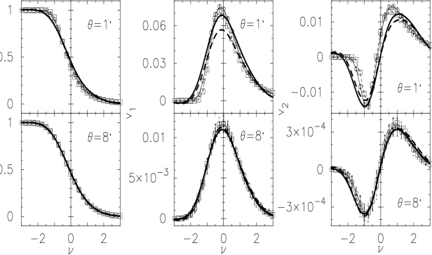
Figure 2: Minkowski functionals, the area fraction (left), circumference (middle), and Euler characteristics (right) per square arcmin for the reconstructed convergence fields with two different smoothing scales of $\theta=1^{\prime}$ (upper) and $\theta=8^{\prime}$ (lower), respectively. Solid (SCDM model) and dashed ($\Lambda$CDM) curves show the analytical predictions of Minkowski functionals calculated by equation (1). The mean values (circles and boxes for SCDM and $\Lambda$CDM models, respectively) and the error bars in each bin of $\nu$ are estimated from the ten different realizations with the area of $3\times 3$ square degrees.

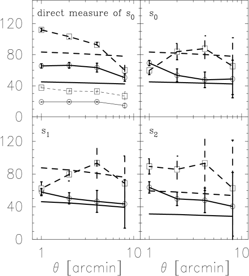
Figure 3: The directly measured value of skewness parameter (top left) from the simulated convergence maps, and the skewness parameters $s_{0}$ (top right), $s_{1}$ (bottom left), and $s_{2}$ (bottom right) estimated from fitting between the simulated Minkowski functionals and their analytical predictions. In each panel, solid lines with and without circle symbols represent the results by simulation and by the perturbation theory, respectively, in SCDM model, while dashed lines with and without box symbols are results in $\Lambda$CDM model. The error bars are estimated from ten realizations for the observation field with $9^{\circ}\times 9^{\circ}$ area (see text in detail). In addition, in top left panel thin lines represent the direct measure of $s_{0}$ in the same range of $-1.5\leq\nu\leq 1.5$ as used in the Minkowski functionals method.

Table 1: Summary of the parameters used for the N-body simulations. $h$ is the Hubble constant in units of $100\,{\rm km\,s^{-1}\,Mpc^{-1}}$.

Model	$\Omega_{m}$	$\Omega_{\Lambda}$	$\Gamma$	$\sigma_{8}$	m${}_{\rm{p}}(h^{-1}M_{\odot})$)
SCDM	1.0	0.0	0.5	0.6	1.7$\times$1010
$\Lambda$CDM	0.3	0.7	0.21	1.0	5.0$\times$109

Table 2: The value of $\Omega_{m}$ estimated from the direct measurement of $s_{0}$ and from the measurements of $s_{0}$ and $s_{1}$ through the fitting of Minkowski functionals for simulation data with $\theta=2^{\prime},4^{\prime}$ and $8^{\prime}$. We here employed the flat universe models with $\Omega_{m}+\Omega_{\Lambda}=1$.

Model	$\Omega_{m}$ from the direct measure of $s_{0}$	$\Omega_{m}$ from Minkowski functionals
SCDM ($\Omega_{m}=1.0$)	0.50 $\pm$ 0.19	0.78 $\pm$ 0.22
$\Lambda$CDM ($\Omega_{m}=0.3$)	0.24 $\pm$ 0.05	0.31 $\pm$ 0.07

References

- Bacon, Refregier & Ellis (2000) Bacon, D., Refregier, A. & Ellis, R., 2000, MNRAS, 318, 625B
- Bardeen et al. (1986) Bardeen, J. M., Bond, J. R., Kaiser, N., & Szalay, A. S., 1986, ApJ, 304, 15
- Bernardeau, van Waerbeke & Mellier (1997) Bernardeau, F., van Waerbeke, L., & Mellier, Y., 1997, A&A, 322, 1
- Blandford et al. (1991) Blandford, R. D., Saust, R. D., Brainerd, A. B., & Villumsen, J. V., 1991, MNRAS, 251, 600
- Gott, Melott & Dickinson (1986) Gott, J. R., Melott, A. L, & Dickinson, M., 1986, ApJ, 306, 341
- (6) Hamana, T., Martel, H., & Futamase, T., 2000, ApJ, 529, 56
- (7) Hamana, T., Colombi, S. T., Thion, A., Devrient, J. E. G. T., Mellier, Y., & Bernardeau, F., 2000, (astro-ph/0012200)
- Hui (1999) Hui, L. 1999, ApJ, 519, 9
- Jain, Seljak & White (2000) Jain, B., Seljak, U., & White, S., 2000, ApJ, 530, 547
- Jing (1998) Jing, Y. P., 1998, ApJ, 503, L9
- Jing & Fang (1994) Jing, Y. P., & Fang, L. Z., 1994, ApJ, 432, 438
- Kaiser (1992) Kaiser, N., 1992, ApJ, 388, 272
- Kaiser, Willson & Luppino (2000) Kaiser, N., Willson, G. & Luppino, G. A., 2000, (astro-ph/0003338)
- Maoli et al. (2000) Maoli, R., et al., 2000, (astro-ph/0011251)
- Matsubara (2000) Matsubara, T., 2000, (astro-ph/0006269)
- Matsubara & Jain (2000) Matsubara, T. & Jain, B., 2000, (astro-ph/0009402)
- Miralda-Escude (1991) Miralda-Escude, J., 1991, ApJ, 380, 1
- Scoccimarro & Frieman (1999) Scoccimarro, R., & Frieman, J., 1999, ApJ, 520, 35
- Schmalzing & Buchert (1997) Schmalzing, J., & Buchert, T., 1997, ApJ, 482, L1
- van Waerbeke et al. (2000) van Waerbeke, L. et al. 2000, A&A, 358, 30
- White & Hu (2000) White, M., & Hu, W., 2000, ApJ, 537, 1
- Winitzki & Kosowsky (1997) Winitzki, S., & Kosowsky, A., 1997, New Astronomy, 3, 75
- Wittman et al. (2000) Wittman, D. M., Tyson, J. A., Kirkman, D., Dell’Antonoio, I., & Bernstein, G., 2000, Nature, 405, 143