Genus statistics for galaxy clusters
and nonlinear biasing of dark matter halos

Abstract

We derive an analytic formula of genus for dark matter halos assuming that the primordial mass density field obeys the random-Gaussian statistics. In particular, we for the first time take account of the nonlinear nature of the halo biasing, in addition to the nonlinear gravitational evolution of the underlying mass distribution. We examine in detail the extent to which the predicted genus for halos depends on the redshift, smoothing scale of the density field, and the mass of those halos in representative cold dark matter models. In addition to the full model predictions, we derive an explicit perturbation formula for the halo genus which can be applied to a wider class of biasing model for dark matter halos. With the empirical relation between the halo mass and the luminosity/temperature of galaxy clusters, our prediction can be compared with the upcoming cluster redshift catalogues in optical and X-ray bands. Furthermore, we discuss the detectability of the biasing and cosmological model dependence from the future data.

1 INTRODUCTION

The genus statistics is a quantitative measure of the topological nature of the density field. In contrast to the more conventional two-point statistics like the two-point correlation functions and the power spectrum, genus is sensitive to the phase information of the density field, and therefore plays a complementary role in characterizing the present cosmic structure.

Mathematically, genus $G(\nu)$ is defined as $-1/2$ times the Euler characteristic of the isodensity contour of the density field at the level of $\nu$ times the rms fluctuations $\sigma$. In practice this is equal to (number of holes) $-$ (number of isolated regions) of the isodensity surface. In cosmology it is convenient to use the genus per unit volume, or the genus density $g(\nu)$, rather than the genus itself. The genus density of the random-Gaussian density field is analytically given by

$$g(\nu)=\frac{1}{(2\pi)^{2}}\left(\frac{\sigma_{1}^{2}}{3\sigma^{2}}\right)^{3/2}(1-\nu^{2})\exp\left(-\frac{\nu^{2}}{2}\right),$$ (1)

where $\sigma_{1}\equiv\langle[\nabla\delta(x)]^{2}\rangle$ and $\sigma\equiv\langle[\delta(x)]^{2}\rangle$ with $\langle\rangle$ denoting the average over the probability distribution function (PDF) of the density field (Doroshkevich 1970; Adler 1981; Bardeen et al. 1986; Gott, Melott, & Dickinson 1986; Hamilton, Gott, & Weinberg 1986).

In fact the standard model of structure formation assumes that the primordial density field responsible for the current cosmic structure is random-Gaussian. Thus equation (1) is the most important analytical result for genus, and has been compared with the observational estimates from galaxy and cluster samples in order to probe the random-Gaussianity in the primordial density field (e.g., Vogeley et al. 1994; Rhoads et al. 1994; Canavezes et al. 2000). Nevertheless the nonlinear gravitational evolution inevitably changes the random-Gaussianity. Matsubara (1994) explicitly finds the next-order terms for the genus using the perturbation analysis of the evolution of the density field. His formula is in good agreement with the results from N-body simulations (Matsubara & Suto 1996; Colley et al. 2000) in a weakly nonlinear regime. The genus in a strongly nonlinear regime has been considered using a variety of modelings including the direct numerical simulations (Matsubara & Suto 1996), the empirical log-normal PDF for cosmological nonlinear density field (Matsubara & Yokoyama 1996), and the Zel’dovich approximation (Seto et al. 1997).

Those previous studies, however, did not take account of the effect of biasing between luminous objects and dark matter. On the other hand, there is growing evidence that the biasing is described by a nonlinear and stochastic function of the underlying mass density (Dekel & Lahav 1999). If this is the case, the genus for the isodensity surface of luminous objects should be significantly different from that of mass. Of course the biasing is supposed to be very dependent on the specific objects, and the general prediction is virtually impossible. Therefore in this paper we focus on a nonlinear stochastic biasing model of dark matter halos (Taruya & Suto 2000). This model is based on the extended Press-Schechter theory (e.g., Bower 1991; Bond et al. 1991) combined with the Mo & White (1996) bias formula, and is in reasonable agreement with numerical simulations (Kravtsov & Klypin 1999; Somerville et al. 2001; Yoshikawa et al. 2001). In this paper, we present an analytic expression for genus of dark matter halos by taking account of the nonlinearity in the halo biasing. Since recent numerical simulations (Taruya et al. 2001) suggest the stochasticity in halo biasing is fairly small on scales $\lower 2.15277pt\hbox{$\;\buildrel>\over{\sim}\;$}10h^{-1}$Mpc (see their Fig.8), we neglect the effect of stochasticity in what follows. The one-to-one correspondence between those halos and galaxy clusters is a fairly standard assumption, and our predictions for halo genus as a function of halo mass can be translated into those of clusters with the corresponding luminosity/temperature. Therefore our predictions are useful in future data analysis of the cluster surveys in different bands.

The plan of this paper is as follows. In §2, we briefly review the nonlinear stochastic biasing model for dark matter halos that we adopt, and derive an analytic expression of genus for halos. In §3, we present specific predictions of genus statistics paying particular attention to the dependence on the smoothing length, the range of halo mass, cosmological parameters and the redshift. Finally §4 is devoted to conclusions and discusses implications of our results.

2 PREDICTING THE GENUS FOR HALOS

In this section we derive an analytic expression for genus of halos adopting the nonlinear stochastic biasing model (Taruya & Suto 2000). First we briefly review the halo biasing model (§2.1). Assuming that PDF of nonlinear mass fluctuations is given by the log-normal distribution, we compute the PDF of halo number density fluctuations, $P_{\rm halo}({\delta_{\rm halo}})$ (§2.2). Finally in §2.3 we present our analytic expression for genus of halos which properly takes account of both the biasing and the nonlinear gravitational evolution for the first time.

2.1 Halo Biasing Model

The central idea of the halo biasing model of Taruya & Suto (2000) is to regard the formation epoch and mass of halos as the major two hidden (unobservable) variables which lead to the nonlinear stochastic behavior of the halo number density field, ${\delta_{\rm halo}}$, as a function of the underlying mass density fluctuation, ${\delta_{\rm mass}}$. Applying the extended Press-Schechter theory, Mo & White (1996) derived an expression of ${\delta_{\rm halo}}$ at $z$ smoothed over the scale of ${R_{\rm\scriptscriptstyle S}}$ as a function of ${\delta_{\rm mass}}$, the halo mass $M$, and its formation epoch ${z_{\rm f}}$:

$${\delta_{\rm halo}}={\Delta_{\rm h}}({R_{\rm\scriptscriptstyle S}},z|{\delta_{\rm mass}},M,{z_{\rm f}}).$$ (2)

Since the above procedure assumes the spherical collapse model, we adopt the top-hat smoothing in computing ${\delta_{\rm mass}}$ and ${\delta_{\rm halo}}$ throughout the paper. Convolving the above expression with the Press–Schechter mass function $n(M,z;\delta_{\rm c,0})$ and the halo formation epoch distribution function, $\partial p/\partial{z_{\rm f}}({z_{\rm f}}|M,z)$ (Lacey & Cole 1993; Kitayama & Suto 1996), Taruya & Suto (2000) derive the following conditional PDF of ${\delta_{\rm halo}}$ for a given ${\delta_{\rm mass}}$, $P({\delta_{\rm halo}}|{\delta_{\rm mass}})$:

$$P({\delta_{\rm halo}}|{\delta_{\rm mass}})~{}d{\delta_{\rm halo}}~{}=~{}{\cal N}^{-1}~{}\int\int_{{\cal C}(M,{z_{\rm f}})}dM~{}d{z_{\rm f}}~{}~{}\frac{\partial p}{\partial{z_{\rm f}}}({z_{\rm f}}|M,z)~{}n(M,z;\delta_{\rm c,0}),$$ (3)

where $\delta_{\rm c,0}$ is the critical threshold for spherical collapse $3(12\pi)^{3/2}/20\simeq 1.69$. The region of the integration, ${\cal C}(M,{z_{\rm f}})$, is given as follows:

$${\cal C}(M,{z_{\rm f}})=\{~{}(M,{z_{\rm f}})~{}|~{}{\delta_{\rm halo}}\leq~{}{\Delta_{\rm h}}({R_{\rm\scriptscriptstyle S}},z|{\delta_{\rm mass}},M,{z_{\rm f}})~{}\leq{\delta_{\rm halo}}+d{\delta_{\rm halo}},$$ (4)

$$M_{\rm min}\leq M\leq M_{\rm max},\quad z\leq{z_{\rm f}}\leq\infty~{}\},$$ (5)

where $M_{\rm min}$ and $M_{\rm max}$ denote maximum and minimum of halo mass. The normalization factor ${\cal N}$ is defined as

$${\cal N}=\int_{M_{\rm min}}^{M_{\rm max}}dM\int_{z}^{\infty}d{z_{\rm f}}~{}~{}\frac{\partial p}{\partial{z_{\rm f}}}({z_{\rm f}}|M,z)~{}n(M,z;\delta_{\rm c,0}).$$ (6)

The joint PDF $P({\delta_{\rm mass}},{\delta_{\rm halo}})$ is simply given by multiplying the PDF of ${\delta_{\rm mass}}$, $P({\delta_{\rm mass}})$, which we assume is log-normal:

$$P({\delta_{\rm mass}},{\delta_{\rm halo}})=P({\delta_{\rm halo}}|{\delta_{\rm mass}})\,P({\delta_{\rm mass}}).$$ (7)

It is well known that the PDF of the nonlinear mass density field is approximated by the log-normal distribution (e.g. Coles & Jones 1991; Kofman et al. 1994). Using this PDF in the present context, however, implies that we implicitly assume the one-to-one correspondence of the primordial density fluctuation and the evolved nonlinear one (${\delta_{\rm mass}}$). Recently Kayo et al. (2001) show that the scatter around the mean relation between the initial and final density fluctuations is significant although the nonlinear PDF is in good agreement with the log-normal. Thus it should be noted that the present paper neglects the effect of the scatter or the stochasticity of the mass density field. This effect will be examined elsewhere when we compare the predictions of this paper with results of N-body simulations (Hikage et al. in preparation). In the same spirit, we below do not take into account the stochasticity of ${\delta_{\rm halo}}$ with respect to ${\delta_{\rm mass}}$, and adopt the one-to-one mapping between ${\delta_{\rm halo}}$ and ${\delta_{\rm mass}}$ represented by the mean biasing:

$$\overline{{\delta_{\rm halo}}}=\int P({\delta_{\rm halo}}|{\delta_{\rm mass}})~{}{\delta_{\rm halo}}~{}d{\delta_{\rm halo}}~{}\equiv f_{\rm bias}({\delta_{\rm mass}}).$$ (8)

In what follows, we use ${\delta_{\rm halo}}$ to indicate $\overline{{\delta_{\rm halo}}}({\delta_{\rm mass}})=f_{\rm bias}({\delta_{\rm mass}})$ in reality.

In §3.2, we show that our results can be well reproduced from the mean biasing function up to the second-order term of ${\delta_{\rm mass}}$. In fact, this is important in the sense that our genus expression in the next section is applicable to the more general biasing scheme as long as its second-order parameterization form is specified. In the present biasing model, we first compute the mean biasing numerically according to equation (8), and then fit the data in the range of $-0.1<{\delta_{\rm mass}}<0.1$ to the following quadratic model:

$$f_{\rm bias}^{\rm fit(2)}({\delta_{\rm mass}})=b_{1}{\delta_{\rm mass}}+\frac{b_{2}}{2}({\delta_{\rm mass}}^{2}-{\sigma_{\rm mm}}^{2})$$ (9)

which satisfy the relation $\langle f_{\rm bias}^{\rm fit(2)}({\delta_{\rm mass}})\rangle=0$ (${\sigma_{\rm mm}}$ is defined in eq.[11] below). The fitted values for the linear and the second-order biasing coefficients, $b_{\rm 1}$ and $b_{\rm 2}$, are listed in Table 1 for several models.

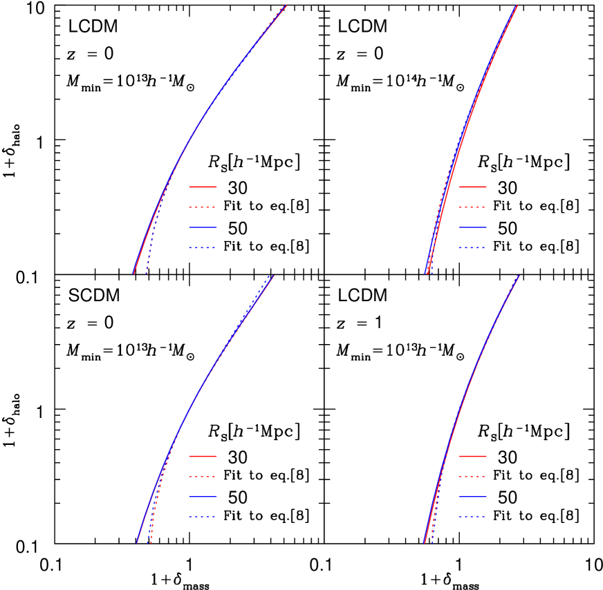
Figure 1: The mean biasing function $f_{\rm bias}({\delta_{\rm mass}})$(solid) and its fitting up to the second-order of ${\delta_{\rm mass}}$, $f_{\rm bias}^{\rm fit(2)}({\delta_{\rm mass}})$(dotted). The red and blue lines indicate the results with ${R_{\rm\scriptscriptstyle S}}=30h^{-1}$Mpc and $50h^{-1}$Mpc. Upper-left: LCDM model, $z=0$, and $M_{\rm min}=10^{13}h^{-1}M_{\odot}$ ; Upper-right: LCDM model, $z=0$, and $M_{\rm min}=10^{14}h^{-1}M_{\odot}$ ; Lower-left: SCDM model, $z=0$, and $M_{\rm min}=10^{13}h^{-1}M_{\odot}$ ; Lower-right: LCDM model, $z=1$, and $M_{\rm min}=10^{13}h^{-1}M_{\odot}$. We set $M_{\rm max}=10^{16}h^{-1}M_{\odot}$.

Figure 1 plots $f_{\rm bias}({\delta_{\rm mass}})$ and $f_{\rm bias}^{\rm fit(2)}({\delta_{\rm mass}})$ in solid and dotted lines, for different $M_{\rm min}$, ${R_{\rm\scriptscriptstyle S}}$, and $z$. Since we are primarily interested in the galaxy cluster scales, we consider the following values of the parameters; the minimum mass of halo $M_{\rm min}=10^{13}h^{-1}M_{\odot}$ and $10^{14}h^{-1}M_{\odot}$, the smoothing length ${R_{\rm\scriptscriptstyle S}}=30h^{-1}{\rm Mpc}$ and $50h^{-1}{\rm Mpc}$, $z=0$ and $1$ ($h$ denotes the Hubble constant in units of 100 km$\cdot$s${}^{-1}\cdot$Mpc^-1). While we set the maximum halo mass $M_{\rm max}=10^{16}h^{-1}M_{\odot}$, the larger value of $M_{\rm max}$ does not change the results below since the number density of such massive halos is quite small. Our predictions below are computed in two representative Cold Dark Matter (CDM) models; Lambda CDM (LCDM) with ($\Omega_{0},\lambda_{0},\sigma_{8},h$) = (0.3,0.7,1.0,0.7), and Standard CDM (SCDM) with ($\Omega_{0},\lambda_{0},\sigma_{8},h$)=(1.0,0.0,0.6,0.5). The density parameter $\Omega_{0}$, dimensionless cosmological constant, $\lambda_{0}$, and the top-hat mass fluctuation at $8h^{-1}$Mpc, $\sigma_{8}$ are normalized according to the cluster abundance (Kitayama & Suto 1997).

Figure 1 clearly indicates the degree of nonlinearity in our biasing model. For the range of parameter values of our interest, the quadratic fit $f_{\rm bias}^{\rm fit(2)}$ provides a reasonable approximation to the mean biasing. As $M_{\rm min}$ and $z$ increase, nonlinearity in the biasing becomes stronger (see $b_{\rm 2}$ in Table 1 ), and one expects the more significant departure of the resulting genus density from the random-Gaussian prediction (eq.[1]) as we will show below.

2.2 Probability Distribution Function of Nonlinear Mass and Halo Density Fields

PDF of the objects of interest is the most important and basic statistics in computing their genus. The PDF of halos in our biasing model is derived in this subsection.

Standard models of structure formation inspired by the inflation picture assume that the PDF of the primordial density field obeys the random-Gaussian statistics. While the nonlinear gravitational evolution of the density field distorts the primordial random-Gaussianity, the log-normal PDF is known to be an empirical good approximation to the nonlinear mass density field ${\delta_{\rm mass}}$ (see discussion in the previous subsection):

$$P_{\rm mass}({\delta_{\rm mass}})d{\delta_{\rm mass}}=\frac{1}{(1+{\delta_{\rm mass}})\sqrt{2\pi\ln(1+{\sigma_{\rm mm}}^{2})}}\exp\left[-\frac{\{\ln[(1+{\delta_{\rm mass}})\sqrt{1+{\sigma_{\rm mm}}^{2}}]\}^{2}}{2\ln(1+{\sigma_{\rm mm}}^{2})}\right]d{\delta_{\rm mass}}.$$ (10)

The variance ${\sigma_{\rm mm}}({R_{\rm\scriptscriptstyle S}},z)$ of the mass fluctuations at $z$ smoothed over the scale ${R_{\rm\scriptscriptstyle S}}$ is computed from the nonlinear power spectrum $P(k,z)$ convolved with the specific window function $W^{2}(k{R_{\rm\scriptscriptstyle S}})$:

$${\sigma_{\rm mm}}^{2}({R_{\rm\scriptscriptstyle S}},z)=\int\frac{dk}{2\pi^{2}}k^{2}P_{\rm nl}(k,z)W^{2}(k{R_{\rm\scriptscriptstyle S}})~{}.$$ (11)

In what follows, we adopt the fitting formula of the nonlinear CDM power spectrum $P_{\rm nl}(k,z)$ (Peacock & Dodds 1996). Throughout the paper, we adopt the top-hat window function:

$$W(x)=\frac{3}{x^{3}}(\sin{x}-x\cos{x}).$$ (12)

The resulting PDF in this prescription proves to be in excellent agreement with N-body simulation results (Kayo et al. 2001).

One interpretation of equation (10) is that the nonlinear mass density field ${\delta_{\rm mass}}$ has the following one-to-one mapping from a random-Gaussian field ${\delta_{\rm\scriptscriptstyle RG}}$ with unit variance:

$${\delta_{\rm mass}}=f_{\rm ln}[{\delta_{\rm\scriptscriptstyle RG}}]=\frac{1}{\sqrt{1+{\sigma_{\rm mm}}^{2}}}~{}\exp~{}[\sqrt{\ln(1+{\sigma_{\rm mm}}^{2})}{\delta_{\rm\scriptscriptstyle RG}}]-1.$$ (13)

Physically speaking, the above ${\delta_{\rm\scriptscriptstyle RG}}$ corresponds to the primordial density field apart from the arbitrary normalization factor. Of course this mapping cannot be strict since ${\delta_{\rm mass}}$ should not be determined locally. Nevertheless this interpretation provides an interesting and useful method to compute genus of nonlinear mass density field as discussed by Matsubara & Yokoyama (1996).

We extend this idea in our biasing model. Since our halo density field is given by the mean biasing (8) and we adopt the log-normal PDF (10) for ${\delta_{\rm mass}}$, we can easily obtain the PDF for ${\delta_{\rm halo}}=f_{\rm bias}({\delta_{\rm mass}})=f_{\rm bias}(f_{\rm ln}({\delta_{\rm\scriptscriptstyle RG}}))$ as follows:

$$P_{\rm halo}({\delta_{\rm halo}})d{\delta_{\rm halo}} = P_{\rm mass}[f^{-1}_{\rm bias}({\delta_{\rm halo}})]\left.{d{\delta_{\rm mass}}\over d\,f_{\rm bias}({\delta_{\rm mass}})}\right|_{{\delta_{\rm mass}}=f^{-1}_{\rm bias}({\delta_{\rm halo}})}d{\delta_{\rm halo}}$$

$$= \frac{1}{f^{\prime}_{\rm bias}(f_{\rm bias}^{-1}({\delta_{\rm halo}}))(1+f_{\rm bias}^{-1}({\delta_{\rm halo}}))\sqrt{2\pi\ln(1+{\sigma_{\rm mm}}^{2})}}$$

$$\times \exp\left[-\frac{\{\ln[(1+f_{\rm bias}^{-1}({\delta_{\rm halo}}))\sqrt{1+{\sigma_{\rm mm}}^{2}}]\}^{2}}{2\ln(1+{\sigma_{\rm mm}}^{2})}\right]d{\delta_{\rm halo}}.$$ (15)

In the above, $f^{\prime}_{\rm bias}({\delta_{\rm mass}})$ denotes the derivative respect to ${\delta_{\rm mass}}$, and $f^{-1}_{\rm bias}$ is the inverse of the monotonic function $f_{\rm bias}$.

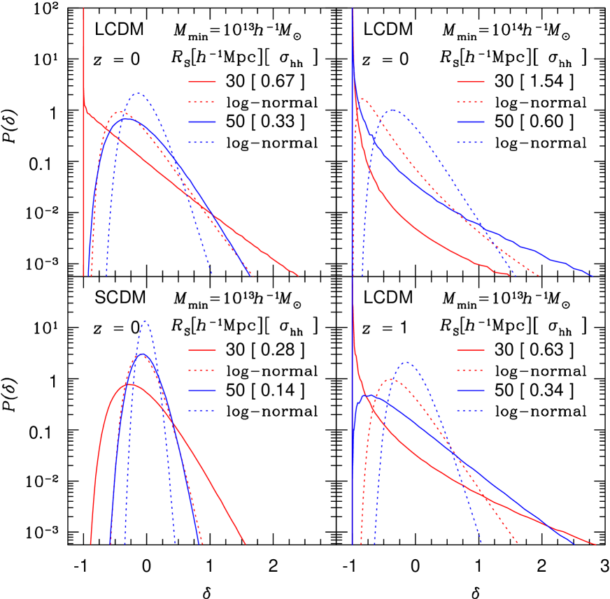
Figure 2: Probability distribution functions for dark halos with ${R_{\rm\scriptscriptstyle S}}=30h^{-1}$Mpc and $50h^{-1}$Mpc. For reference, dotted lines indicate the log-normal distribution with the variance of the corresponding ${\sigma_{\rm hh}}$. Upper-left: LCDM model, $z=0$, and $M_{\rm min}=10^{13}h^{-1}M_{\odot}$ ; Upper-right: LCDM model, $z=0$, and $M_{\rm min}=10^{14}h^{-1}M_{\odot}$ ; Lower-left: SCDM model, $z=0$, and $M_{\rm min}=10^{13}h^{-1}M_{\odot}$ ; Lower-right: LCDM model, $z=1$, and $M_{\rm min}=10^{13}h^{-1}M_{\odot}$. In all panels $M_{\rm max}=10^{16}h^{-1}M_{\odot}$.

Figure 2 plots the PDF for dark halos in solid lines, respectively, employing the same sets of parameters as Figure 1. In order to separate the changes of the PDF due to the nonlinear biasing and the nonlinear gravitational evolution, we compare the dark halo PDF with the log-normal PDF (eq:[10]; dotted lines). Also for that purpose the variance ${\sigma_{\rm mm}}$ of the log-normal in equation (10) is adjusted to the corresponding ${\sigma_{\rm hh}}$ of the halos:

$${\sigma_{\rm hh}}^{2}\equiv\int\int{\delta_{\rm halo}}^{2}P({\delta_{\rm mass}},{\delta_{\rm halo}})d{\delta_{\rm mass}}d{\delta_{\rm halo}},$$ (16)

in plotting the log-normal PDF curves, Note that the quantity $\sigma_{\rm hh}$ is somewhat different from variance of the averaged biasing, $\langle[\overline{\delta_{\rm halo}}({\delta_{\rm mass}})]^{2}\rangle$ and contains the nonlinearity and the stochasticity of biasing.

Figure 2 shows the sensitivity of PDFs for the halo mass $M_{\rm min}$ and the cosmological parameters, especially for the fluctuation amplitude $\sigma_{8}$. The dark halo PDF significantly differs from the log-normal PDF even using the same value of variance, which clearly indicates the importance of the nonlinearity in the halo biasing. In some models, the PDF at ${\delta_{\rm halo}}=-1$ diverges since ${\delta_{\rm halo}}$ in our model reaches $-1$ even though ${\delta_{\rm mass}}$ is greater than $-1$. Then $f_{\rm bias}$ is not a one-to-one mapping between ${\delta_{\rm halo}}$ and ${\delta_{\rm mass}}$ and the expression (2.2) becomes singular there. Of course, this divergence occurs only at ${\delta_{\rm halo}}=-1$, and does not affect our results for ${\delta_{\rm halo}}>-1$.

2.3 Genus Curve For Dark Halos

As we describe in the previous subsection, our halo biasing model results in the one-to-one mapping between ${\delta_{\rm\scriptscriptstyle RG}}$ and ${\delta_{\rm halo}}=f_{\rm bias}({\delta_{\rm mass}})=f_{\rm bias}(f_{\rm ln}({\delta_{\rm\scriptscriptstyle RG}}))$. Then using the prescription of Matsubara & Yokoyama (1996), we can derive the genus density explicitly.

For the nonlinear mass density ${\delta_{\rm mass}}$ with the log-normal PDF (10), the genus density is computed as (Matsubara & Yokoyama 1996):

$$g_{\rm mass}(\nu_{\rm m}) = {g_{\rm\scriptscriptstyle MAX}}~{}\exp\left[-\frac{\{\ln[(1+\nu_{\rm m}{\sigma_{\rm mm}})\sqrt{1+{\sigma_{\rm mm}}^{2}}]\}^{2}}{2\ln(1+{\sigma_{\rm mm}}^{2})}\right]$$ (17)

$$\times \left[1-\frac{\{\ln[(1+\nu_{\rm m}{\sigma_{\rm mm}})\sqrt{1+{\sigma_{\rm mm}}^{2}}]\}^{2}}{\ln(1+{\sigma_{\rm mm}}^{2})}\right],$$

where the level of isodensity contour $\nu_{\rm m}$ is given by $\delta_{\rm mass}/\sigma_{\rm mm}$. The quantity ${g_{\rm\scriptscriptstyle MAX}}$ is the maximum value of the genus:

$${g_{\rm\scriptscriptstyle MAX}}=g_{\rm mass}(\delta_{\rm\scriptscriptstyle MAX}/{\sigma_{\rm mm}})=\frac{1}{(2\pi)^{2}}\frac{\sigma^{3}_{\rm 1,m}}{[3(1+{\sigma_{\rm mm}}^{2})\ln(1+{\sigma_{\rm mm}}^{2})]^{3/2}},$$ (18)

at $\delta_{\rm\scriptscriptstyle MAX}\equiv 1/\sqrt{1+{\sigma_{\rm mm}}^{2}}-1$ with

$$\sigma_{\rm 1,m}^{2}({R_{\rm\scriptscriptstyle S}},z)=\int\frac{dk}{2\pi^{2}}k^{4}P_{\rm nl}(k,z)W^{2}(k{R_{\rm\scriptscriptstyle S}})~{}.$$ (19)

We transform this genus density using the mean biasing relation ${\delta_{\rm halo}}=f_{\rm bias}({\delta_{\rm mass}})$. Then, at a given threshold $\nu_{\rm h}\equiv\delta_{\rm halo}/\sigma_{\rm hh}$, our final expression for the genus density of dark halos becomes as follows:

$$g_{\rm halo}(\nu_{\rm h}) = {g_{\rm\scriptscriptstyle MAX}}~{}\exp\left[-\frac{\{\ln[(1+f_{\rm bias}^{-1}(\nu_{\rm h}{\sigma_{\rm hh}}))\sqrt{1+{\sigma_{\rm mm}}^{2}}]\}^{2}}{2\ln(1+{\sigma_{\rm mm}}^{2})}\right]$$ (20)

$$\times \left[1-\frac{\{\ln[(1+f_{\rm bias}^{-1}(\nu_{\rm h}{\sigma_{\rm hh}}))\sqrt{1+{\sigma_{\rm mm}}^{2}}]\}^{2}}{\ln(1+{\sigma_{\rm mm}}^{2})}\right],$$

with $\sigma_{\rm hh}$ defined by (15). Here, ${g_{\rm\scriptscriptstyle MAX}}=g_{\rm halo}[f_{\rm bias}(\delta_{\rm\scriptscriptstyle MAX})/{\sigma_{\rm hh}}]=g_{\rm mass}(\delta_{\rm\scriptscriptstyle MAX}/{\sigma_{\rm mm}})$ is given also by equation (18) and is listed in Table 2 for some models.

3 PREDICTIONS OF GENUS FOR HALOS IN CDM MODELS

In this section we present several model predictions of the genus density for dark matter halos with particular emphasis on its parameter dependence. Then we examine to which extent our predictions are reproduced with a perturbation model on the nonlinear gravitational growth and the biasing.

3.1 Parameter Dependence of the Halo Genus

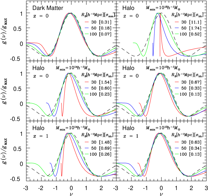
Figure 3: Normalized genus density $g(\nu)/{g_{\rm\scriptscriptstyle MAX}}$ for dark halos in LCDM model with ${R_{\rm\scriptscriptstyle S}}=30h^{-1}$Mpc (red), $50h^{-1}$Mpc (blue), and $100h^{-1}$Mpc (green). For comparison, Upper-left panel plots the normalized genus density for dark matter. The other panels assume ${M_{\rm max}=10^{16}h^{-1}M_{\odot}}$. Upper-right: $z=0$ and ${M_{\rm min}=10^{15}h^{-1}M_{\odot}}$; Middle-left: $z=0$ and ${M_{\rm min}=10^{14}h^{-1}M_{\odot}}$; Middle-right: $z=0$ and ${M_{\rm min}=10^{13}h^{-1}M_{\odot}}$; Lower-left: $z=1$ and ${M_{\rm min}=10^{14}h^{-1}M_{\odot}}$; Lower-right: $z=1$ and ${M_{\rm min}=10^{13}h^{-1}M_{\odot}}$.

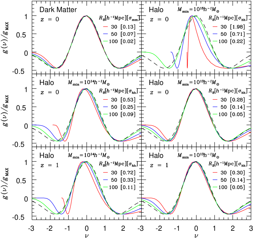
Figure 4: Same as Figure 3 for SCDM model.

Consider the halo mass dependence first. As we argued in §2.1, the maximum mass does not affect the results as long as $M_{\rm max}>10^{16}M_{\odot}$. They are, however, very sensitive to the minimum mass $M_{\rm min}$. This mass dependence is shown in Figures 3 and 4 in LCDM and SCDM models, respectively, where we plot the normalized genus density (i.e., $g(\nu)$ in units of its maximum value ${g_{\rm\scriptscriptstyle MAX}}$). As $M_{\rm min}$ increases, the nonlinearity of both the halo biasing and the mass fluctuation amplitude becomes stronger (see Fig.1 and Table 1) which results in the significant departure from the random-Gaussian prediction (dashed lines).

Also the genus is fairly dependent on the smoothing length ${R_{\rm\scriptscriptstyle S}}$ (Figs 3 and 4, and Table 2). While the genus with ${R_{\rm\scriptscriptstyle S}}\lower 2.15277pt\hbox{$\;\buildrel>\over{\sim}\;$}100{\hbox{$h^{-1}$}{\rm Mpc}}$ approaches the random-Gaussian prediction, the deviation is detectable with smaller ${R_{\rm\scriptscriptstyle S}}$. We discuss the detectability of the signature in the last section.

In contrast, the redshift dependence is rather weak; neither the amplitude and the shape of the genus density evolves much, at least between $z=0$ and $1$ (which is the relevant range of the redshift for galaxy clusters). This is interpreted as a result of the two competing effects; the stronger clustering due to the halo biasing at higher $z$ and the weaker amplitude of the mass fluctuations(see also Taruya & Yamamoto 2001).

The above features apply both to LCDM and SCDM. The comparison of Figures 3 and 4 indicates that the predictions in SCDM model is slightly closer to the random-Gaussian. This is simply because these models are normalized according to the cluster abundance and thus the mass fluctuation amplitude at $z=0$ is smaller in SCDM ($\sigma_{8}=0.6$) than in LCDM ($\sigma_{8}=1.0$).

3.2 Comparison with the Perturbation Analysis

So far we have presented our predictions using the fully nonlinear model of both the halo biasing and the mass fluctuations. As long as galaxy clusters are concerned, however, we are mainly interested in fairly large ${R_{\rm\scriptscriptstyle S}}$. Therefore the perturbation analysis may be a reasonable approximation. This line of studies is pioneered by Matsubara (1994) in the weakly nonlinear evolution of mass density field, and also by Matsubara (2000) including the effect of biasing. We will perform the perturbation analysis of our full model predictions. This attempt is instructive in understanding the origin of the departure from the random-Gaussianity. Also the resulting perturbation formula becomes useful since it is readily applicable to a wide range of the biasing models, in addition to our halo biasing, once their second-order biasing coefficients are given.

Matsubara (1994) derives the analytical formula for the genus of the mass density field up to the lowest-order term in the (linear) mass variance $\sigma$ :

$$g(\nu)\sim-\frac{1}{(2\pi)^{2}}\left(\frac{\sigma_{1}}{\sqrt{3}\sigma}\right)^{3/2}\exp\left(-\frac{\nu^{2}}{2}\right)\left\{H_{2}(\nu)+\left[\frac{S^{(0)}}{6}H_{5}(\nu)+S^{(1)}H_{3}(\nu)+S^{(2)}H_{1}(\nu)\right]\sigma\right\},$$ (21)

where $S^{(a)}$ represents the skewness parameters defined by

$$S^{(0)} = \frac{\langle\nu^{3}\rangle}{\sigma},$$ (22)

$$S^{(1)} = -\frac{3}{4}\frac{\langle\nu^{2}(\nabla^{2}\nu)\rangle\sigma}{\sigma_{1}^{2}},$$ (23)

$$S^{(2)} = -\frac{9}{4}\frac{\langle(\nabla\nu\cdot\nabla\nu)(\nabla^{2}\nu)\rangle\sigma^{3}}{\sigma_{1}^{4}}.$$ (24)

We expand equation (17) with respect to ${\sigma_{\rm mm}}$ and find that it reduces to

$$g_{\rm mass}(\nu_{\rm m})=g_{\rm\scriptscriptstyle RG}(\nu_{\rm m})\left\{1+\frac{1}{2}H_{3}(\nu_{\rm m}){\sigma_{\rm mm}}+{\cal O}({\sigma_{\rm mm}}^{2})\right\},$$ (25)

where

$$g_{\rm\scriptscriptstyle RG}(\nu_{\rm m})=\frac{1}{(2\pi)^{2}}\left(\frac{\sigma^{2}_{\rm 1,m}}{3\sigma^{2}_{\rm m}}\right)^{3/2}\exp\left(-\frac{\nu_{\rm m}^{2}}{2}\right)(1-\nu_{\rm m}^{2}).$$ (26)

This implies that all the above skewness parameters are equal to 3 in the log-normal PDF.

If we further include the halo biasing effect using the second-order fit ${\delta_{\rm halo}}=f_{\rm bias}^{\rm fit(2)}({\delta_{\rm mass}})$ given by equation (9), we obtain the perturbation formula of our halo genus up to ${\sigma_{\rm hh}}$ as

$$g_{\rm halo}(\nu_{\rm h})=g_{\rm halo,0}(\nu_{\rm h})\left\{1+\frac{1}{2}\frac{b_{1}+b_{2}}{b_{1}b_{\rm var}}H_{3}\left(\frac{b_{\rm var}\nu_{\rm h}}{b_{1}}\right){\sigma_{\rm hh}}+{\cal O}({\sigma_{\rm hh}}^{2})\right\},$$ (27)

where

$$g_{\rm halo,0}(\nu_{\rm h})=\frac{1}{(2\pi)^{2}}\left(\frac{\sigma^{2}_{\rm 1,m}}{3\sigma^{2}_{\rm m}}\right)^{3/2}\exp\left\{-\frac{1}{2}\left(\frac{b_{\rm var}\nu_{\rm h}}{b_{1}}\right)^{2}\right\}\left\{1-\left(\frac{b_{\rm var}\nu_{\rm h}}{b_{1}}\right)^{2}\right\},$$ (28)

with $b_{\rm var}={\sigma_{\rm hh}}/{\sigma_{\rm mm}}$ (Table 1).

If the biasing is linear and deterministic, $b_{\rm var}=b_{1}$ and the skewness parameters reduce to

$$S_{\rm h}^{(0)}=S_{\rm h}^{(1)}=S_{\rm h}^{(2)}=\frac{3}{b_{1}}\left(1+\frac{b_{2}}{b_{1}}\right),$$ (29)

which agrees with equation [4.82] of Matsubara (2000).

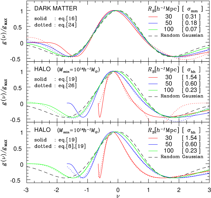
Figure 5: Comparison of $g(\nu)/{g_{\rm\scriptscriptstyle MAX}}$ between the full and perturbation models. The predictions assume $z=0$ in LCDM model, $M_{\rm min}=10^{14}h^{-1}M_{\odot}$, $M_{\rm max}=10^{16}h^{-1}M_{\odot}$, and three different smoothing scales; ${R_{\rm\scriptscriptstyle S}}=30h^{-1}$Mpc (red), $50h^{-1}$Mpc (blue), and $100h^{-1}$Mpc (green). Top: mass in the log-normal model (solid; eq.[17]) and in the perturbation model (dotted; eq.[25]). Middle: dark halos (solid; eq.[20]) and the perturbation formula of our halo genus with the second-order biasing model (dotted; eq.[27]). Bottom: dark halos (solid; eq.[20]) and the results combining the log-normal mass PDF and the second-order biasing model(dotted; eqs.[9], [20]).

Figure 5 compares those perturbation results with our full model predictions; Top panel shows the normalized genus in the log-normal model (solid lines; eq.[17]) and in the perturbation model (dotted lines; eq.[25]). Dotted lines in Middle panel refer to the results combining the weakly nonlinear evolution model (eq.[25]) and the second-order biasing model (eq.[9]), while in Bottom panel they refer to the results combining the log-normal mass PDF (eq.[17]) and the second-order biasing model (eq.[9]). Those are to be compared with our full predictions (solid lines). In the perturbation results (eqs.[25], [27]) we define ${g_{\rm\scriptscriptstyle MAX}}$ respectively as the maximum value in the set of the plotted genus respectively. This comparison indicates that the second-order biasing model provides a very good approximation for the parameters of interest, also that the lowest-order correction to the nonlinear mass evolution dominates for large smoothing lengths ${R_{\rm\scriptscriptstyle S}}\lower 2.15277pt\hbox{$\;\buildrel>\over{\sim}\;$}50{\hbox{$h^{-1}$}{\rm Mpc}}$. Therefore we conclude that our perturbation formula (27) is in practice a useful and reliable approximation to the genus of galaxy halos, which is applicable even beyond our particular biasing model discussed here.

4 SUMMARY AND DISCUSSION

In the present paper, we have presented an analytic model of genus for dark matter halos adopting the stochastic nonlinear halo biasing model by Taruya & Suto (2000), assuming that the primordial mass density field obeys the random-Gaussian statistics. This is the first attempt to predict the genus statistics simultaneously taking account of the nonlinear nature in the biasing and of the nonlinear gravitational evolution of the underlying mass distribution. In the remainder of this section, we discuss several implications of our model predictions.

First of all, we note that our model applies only for dark matter halos identified according to the spherical collapse model strictly speaking. Nevertheless this picture is now widely accepted as an empirical model for galaxy clusters in the universe. In fact, the excellent agreement between the predicted halo abundance and the observed cluster abundance (e.g., Kitayama & Suto 1997; Suto 2000 and references therein) justifies the empirical one-to-one correspondence between the theoretical halo and the observed cluster in a statistical sense. Adopting this conventional view, our predictions for dark matter halos can be readily translated into those for clusters on the basis of the mass–temperature and mass-luminosity relations at the present epoch, for instance, as

$$k_{\rm\scriptscriptstyle B}T=1.3\left(\frac{\Delta_{\rm c}}{18\pi^{2}}\right)^{1/3}\left(\frac{M}{10^{14}h^{-1}M_{\odot}}\right)^{2/3}\Omega_{0}^{1/3}{\rm keV},$$ (30)

and

$$L_{\rm bol}=1.7\left(\frac{\Delta_{\rm c}}{18\pi^{2}}\right)^{1.1}\left(\frac{M}{10^{14}h^{-1}M_{\odot}}\right)^{2.3}\Omega_{0}^{1.1}10^{42}h^{-2}{\rm erg~{}sec^{-1}},$$ (31)

where $k_{\rm\scriptscriptstyle B}$ is Boltzmann constant and $\Delta_{\rm c}$ is the mean density of a virialized cluster (Kitayama & Suto 1996; Suto et al. 2000). Therefore our model predictions can be tested against future cluster observations in various wavebands.

Next it should be stressed that our current model is based on the one-to-one mapping of the primordial density field that obeys the random-Gaussian statistics. In this approximation, if we express our genus predictions as a function of $\overline{\nu}$ defined through the volume fraction $f$:

$$f=\frac{1}{\sqrt{2\pi}}\int^{\infty}_{\overline{\nu}}\exp\left(-\frac{t^{2}}{2}\right)dt,$$ (32)

they simply reduce to the random-Gaussian prediction (eq.[1]). Most previous studies used this $\overline{\nu}$ in order to remove the (unknown) distortion of the PDF due to the gravitational nonlinear evolution. Nevertheless we prefer to adopt the correct definition of $\nu=\delta/\sigma$ because the departure from the Gaussian prediction (eq.[1]) provides also an important measure of the gravitational nonlinear evolution and the nonlinear biasing in more advanced approach than what we took here. For instance, the perturbative results in weakly nonlinear regime (Matsubara 1994) do not reduce to equation (1) even in terms of $\overline{\nu}$, and also the effect of stochasticity in biasing, which is ignored in the present analysis, would add another feature which violates the simple scaling idea behind the use of $\overline{\nu}$. As we have shown in the present paper, the genus as a function $\nu$ can be a useful probe of the nonlinear gravitational evolution and the biasing of objects and mass, as long as the random-Gaussianity of the primordial density field is correct. The comparison between $g(\overline{\nu})$ and $g(\nu)$ is discussed in detail by Colley et al. (2000).

In our genus model, the overall amplitude of genus for dark halos ${g_{\rm\scriptscriptstyle MAX}}$ depends only on mass density spectrum. Therefore the observed amplitude of the cluster genus may provide direct information on the mass fluctuation in principle. However this fact is heavily dependent on our assumption of one-to-one mapping of density fluctuation in equation (8), and needs to be checked with future numerical simulations.

Finally we briefly discuss the future detectability of the departure of the halo genus from the random-Gaussian prediction. We use the top-hat smoothing ${R_{\rm\scriptscriptstyle S}}=50h^{-1}$ Mpc and compute our model predictions for $M_{\rm min}=10^{13}h^{-1}M_{\odot}$ and $10^{14}h^{-1}M_{\odot}$ in SCDM and LCDM models. Figure 6 plots the total number of genus $G(\nu)$; Upper and Lower panels are normalized so as to roughly correspond to the Sloan Digital Sky Survey (SDSS) spectroscopic and photometric cluster samples, respectively. We do not take into account the light cone effect (Yamamoto & Suto 1999; Suto et al. 1999) but rather show the results at the mean redshift $z=0.1$ and $z=0.3$. Taruya & Yamamoto (2001) find that the light-cone effect is not so significant for genus statistics up to $z\sim 1$. The SDSS is expected to detect $N_{\rm spect}\sim 1000$ clusters from spectroscopic data up to $z\sim 0.2$ and $N_{\rm photo}\sim 5000$ from photometric data up to $z\sim 1$. Assuming that errors of genus are dominated by the sampling noise, we assign the error independently of $\nu$ as $\delta G=\sqrt{{g_{\rm\scriptscriptstyle MAX}}V_{\rm eff}}$, where $V_{\rm eff}$ is the effective volume of the sample. We further assume that $V_{\rm eff}$ is proportional to the number of clusters. If we adopt the value for the Abell cluster sample of Rhoads et al.(1994), $\sim 250$ Abell clusters in $V_{\rm eff}=9.5\times 10^{6}\,\,({\hbox{$h^{-1}$}{\rm Mpc}})^{3}$, $V_{\rm eff}$ for SDSS spectroscopic and photometric samples is estimated to be 4 and 20 times larger than that of Rhoads et al.(1994), respectively. The amplitude of the error bars estimated in this way indicates that the departure from the random-Gaussianity should be indeed detectable especially in photometric redshift data and that one can even discriminate among some model predictions with the upcoming data of galaxy clusters.

We plan to improve our model predictions by including the stochasticity in the biasing model, the light-cone effect, and redshift-space distortion. Also we are currently working on evaluating the genus of halos identified from the cosmological N-body simulations. These results and comparison will be reported elsewhere.

Table 1: The linear and second-order biasing coefficients, $b_{1}$ and $b_{2}$(eq.[9]), respectively, and the ratio of the rms fluctuations between dark halos and mass $b_{\rm var}$ ($={\sigma_{\rm hh}}/{\sigma_{\rm mm}}$) for different cosmological models, $z$, $M_{\rm min}$, and ${R_{\rm\scriptscriptstyle S}}$.

Model	$z$	$M_{\rm min}[h^{-1}M_{\rm\odot}]$	${R_{\rm\scriptscriptstyle S}}[h^{-1}{\rm Mpc}]$	$b_{1}$	$b_{2}$	$b_{\rm var}$
LCDM	0	$10^{13}$	30	1.77	0.23	2.12
LCDM	0	$10^{13}$	50	1.76	0.20	1.87
LCDM	0	$10^{13}$	100	1.76	0.14	1.84
LCDM	0	$10^{14}$	30	2.72	3.26	4.90
LCDM	0	$10^{14}$	50	2.92	3.20	3.34
LCDM	0	$10^{14}$	100	3.00	3.70	3.29
SCDM	0	$10^{13}$	30	1.94	0.51	2.07
SCDM	0	$10^{13}$	50	1.94	0.77	2.04
LCDM	1	$10^{13}$	30	2.85	2.78	3.22
LCDM	1	$10^{13}$	50	2.90	2.60	3.08

Table 2: The maximum values of the genus ${g_{\rm\scriptscriptstyle MAX}}$ for different cosmological models, $z$, and ${R_{\rm\scriptscriptstyle S}}$.

Model	$z$	${R_{\rm\scriptscriptstyle S}}[h^{-1}{\rm Mpc}]$	${g_{\rm\scriptscriptstyle MAX}}$[$(100h^{-1}{\rm Mpc})^{-3}$]
LCDM	0	30	4.75
LCDM	0	50	1.49
LCDM	0	100	0.38
LCDM	1	30	3.56
LCDM	1	50	1.13
LCDM	1	100	0.29
SCDM	0	30	9.47
SCDM	0	50	3.83
SCDM	0	100	1.48
SCDM	1	30	7.66
SCDM	1	50	3.12
SCDM	1	100	1.22

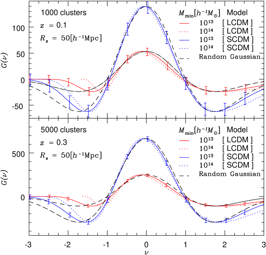
Figure 6: Expected total number of genus for surveys corresponding to $N\simeq 1000$ (Upper panel) and $N\simeq 5000$ (Lower panel); $M_{\rm min}=10^{13}h^{-1}M_{\odot}$ (solid) and $M_{\rm min}=10^{14}h^{-1}M_{\odot}$ (dotted) in LCDM (red) and SCDM (blue) models. All the curves adopt top-hat smoothing of ${R_{\rm\scriptscriptstyle S}}=50{\hbox{$h^{-1}$}{\rm Mpc}}$.

References

- Adler (1981) Adler, R.J. 1981, The Geometry of Random Fields (Chichester: Wiley)
- Bardeen et al. (1986) Bardeen, J.M., Bond, J.R., Kaiser, N., & Szalay, A.S. 1986, ApJ, 304, 15
- Bond et al. (1991) Bond, J.R., Cole, S., Efstathiou, G., & Kaiser, N. 1991, ApJ, 379, 440
- Bower (1991) Bower, R.J. 1991, MNRAS, 248, 332
- Canavezes & Sharpe (2000) Canavezes, A., & Sharpe, J. 2000, MNRAS, submitted (astro-ph/0002405)
- Coles & Jones (1991) Coles, P., & Jones, B. 1991, MNRAS, 248, 1
- Colley et al. (2000) Colley, W.N., Gott III, J.R., Weinberg, D.H., Park, C., & Berlind, A.A. 2000, ApJ, 529, 795
- Dekel & Lahav (1999) Dekel, A., & Lahav, O. 1999, ApJ, 520, 24
- Doroshkevich (1970) Doroshkevich, A.G. 1970, Astrofizika, 6, 581 (English transl. Astrophysics, 6, 320)
- Gott et al. (1986) Gott III, J.R., Mellot, A.L., & Dickinson, M. 1986, ApJ, 306, 341
- Hamilton (1986) Hamilton, A.J.S., Gott III, J.R., & Weinberg, D. 1986, ApJ, 309, 1
- Kayo et al. (2001) Kayo, I., Taruya, A., & Suto, Y. 2001, in preparation
- Kitayama & Suto (1996) Kitayama, T., & Suto, Y. 1996, ApJ, 469, 480
- Kitayama & Suto (1997) Kitayama, T., & Suto, Y. 1997, ApJ, 490, 557
- Kravtsov & Klypin (1999) Kravtsov, A.V., & Klypin, A.A. 1999, ApJ, 520, 437
- Kofman et al. (1994) Kofman, L., Bertschinger, E., Gelb, J.M., Nusser, A., & Dekel, A. 1994, ApJ, 420, 44
- Lacey et al. (1993) Lacey, C., & Coles, S. 1993, MNRAS, 262, 627
- Matsubara (1994) Matsubara, T. 1994, ApJ, 434, L43
- Matsubara (2000) Matsubara, T. 2000, ApJ, submitted (astro-ph/0006269)
- Matsubara & Suto (1996) Matsubara, T., & Suto, Y. 1996, ApJ, 460, 51
- Matsubara & Yokoyama (1996) Matsubara, T., & Yokoyama, J. 1996, ApJ, 463, 409
- Mo et al. (1997) Mo, H., Jing, Y.P., & White, S.D.M. 1997, MNRAS, 284, 189
- Mo & White (1996) Mo, H., & White, S.D.M. 1996, MNRAS, 282, 347
- Park et al. (2000) Park, C., Gott III, J.R., & Choi, Y.J. 2000, ApJ, submitted (astro-ph/0008353)
- Peacock & Dodds (1996) Peacock, J.A., & Dodds, S.J. 1996, MNRAS, 280, L19
- Rhoads et al. (1994) Rhoads, J.E.R., Gott III, J.R., & Postman, M. 1994, ApJ, 421,
- Seto et al. (1997) Seto, N., Yokoyama, J., Matsubara, T., & Siino, M. 1997, ApJ, 110, 177
- Somerville et al. (2001) Somerville, R.S., Lemson, G., Sigad, Y., Dekel, A., Kauffmann, G., & White, S.D.M. 2001, MNRAS, 320, 289
- Suto et al. (1999) Suto, Y., Magira, H., Jing, Y.P., Matsubara, T., & Yamamoto, K. 1999, Prog. Theor. Phys. Suppl., 133, 183
- Suto et al. (2000) Suto, Y., Yamamoto, K., Kitayama, T., & Jing, Y.P. 2000, ApJ, 534, 551
- Suto (2000) Suto, Y. 2000, in Proceedings of the IAP meeting ”Constructing the Universe with Clusters of Galaxies”, edited by Durret, F. & Gerbal, D., in press (astro-ph/0010622)
- Taruya & Suto (2000) Taruya, A., & Suto, Y. 2000, ApJ, 542, 559
- Taruya et al. (2001) Taruya, A., Magira, H., Jing, Y.P., & Suto, Y. 2001, PASJ, 53, in press
- Taruya & Yamamoto (2001) Taruya, A., & Yamamoto, K. 2001, ApJ, 550, April 1 issue, in press
- Vogely et al. (1994) Vogeley, M.S., Park, C., Geller, M.J., Huchra, J.P., & Gott III, J.R. 1994, ApJ, 420, 525
- Yamamoto & Suto (1999) Yamamoto, K., & Suto, Y. 1999, ApJ, 517, 1
- Yoshikawa et al. (2001) Yoshikawa, K., Taruya, A., Jing, Y.P., & Suto. Y. 2001, ApJ, submitted.