Supernovae and the Nature of the Dark Energy

The use of Type Ia supernovae as calibrated standard candles is one of the most powerful tools to study the expansion history of the universe and thereby its energy components. While the analysis of some $\sim$50 supernovae at redshifts around $z\sim$0.5 have provided strong evidence for an energy component with negative pressure, “dark energy”, more data is needed to enable an accurate estimate of the amount and nature of this energy. This might be accomplished by a dedicated space telescope, the SuperNova / Acceleration Probe (snap (2000); SNAP), which aims at collecting a large number of supernovae with $z<2$. In this paper we assess the ability of the SNAP mission to determine various properties of the “dark energy.” To exemplify, we expect SNAP, if operated for three years to study Type Ia supernovae, to be able to determine the parameters in a linear equation of state $w(z)=w_{0}+w_{1}\,z$ to within a statistical uncertainty of $\pm 0.04$ for $w_{0}$ and ${}^{+0.15}_{-0.17}$ for $w_{1}$ assuming that the universe is known to be flat and an independent high precision $(\sigma_{\Omega_{m}}=0.015)$ measurement of the mass density $\Omega_{m}$, is used to constrain the fit. An additional improvement can be obtained if a large number of low-$z$, as well as high-$z$, supernovae are included in the sample.

1 Introduction

The description of the universe lies at the heart of cosmology, and it is not surprising that several methods aiming at the determination of cosmological parameters currently are considered. For example, the power spectrum of the cosmic microwave background radiation provides means to determine the total energy content of the universe, for which recent results of the balloon-based CMB measurements (Jaffe et al. jaffe (2000)) quote the value $\Omega_{\rm tot}=1.05\pm 0.04$. Constraints on the matter energy density of the universe, $\Omega_{m}$, can be derived, e.g., from galaxy cluster abundances (Bahcall & Fan bahcall (1998), Carlberg et al carlberg (1998)), and large-scale structure (Peacock et al 2DF (2001)). These tests are consistent with $\Omega_{m}\sim 0.3$, see however (Blanchard et al. blanchard (2000)). Furthermore, studies of weak lensing effects of background objects in mappings of the sky provides information about the mass distribution in the universe, and thus measures $\Omega_{m}$. See, e.g., van Waerbeke et al. (waerbeke (1999)) for a discussion of the accuracy of this method.

On top of this, measurements of supernovae at various redshifts provide a simple way to estimate cosmological parameters (Goobar & Perlmutter gooperl (1995)). In fact, this is the aim of at least two collaborations (Riess et al. high-z (1998), Perlmutter et al. scp (1999)), both of which recently have published data in favour of a large energy component attributable to a cosmological constant, or an evolving scalar field such as “quintessence” (Ratra & Peebles ratpeeb (1988), Caldwell et al. caldwell (1998)). The feasibility to determine the properties of this “dark energy” component by using supernova data has recently been considered by several authors (see, e.g., Huterer & Turner huturn (1999), Saini et al. saini (2000), Maor et al. maor (2001), Astier astier (2001), Weller & Albrecht welalb (2000) and Barger & Marfatia barmar (2000), just to list a few), and conclusions vary significantly. For instance, Huterer & Turner (huturn (1999)), and Saini et al. (saini (2000)) devise methods for reconstructing the potential of an acceleration-driving scalar field, using supernova measurements. On the other hand, Maor et al. (maor (2001)) assess the possibility to use supernovae to distinguish between various cosmological models, allowing for an evolving equation of state $w(z)$ (which is equivalent to scalar-field models). They conclude that the prospects for determining the equation of state in this way are bleak. Barger & Marfatia (barmar (2000)) support this latter view, exemplifying how particular data realisations may give misleading conclusions regarding the dark energy. Again, Weller & Albrecht (welalb (2000)) are more optimistic regarding a determination of $w(z)$, provided that accurate independent estimates of the matter energy density $\Omega_{m}$ are at hand. As already emphasized by one of us (Astier astier (2001)), much of the discrepancies stem from differences in the initial assumptions, e.g., in the prior knowledge of $\Omega_{m}$.

In this paper we intend to study the extent to which properties of the dark energy can be determined, assuming that observations of a large number of supernovae at high redshifts become available. Such data could be provided by the projected SNAP satellite mission. In section 2 we establish our notation and give the expression for the luminosity distance $d_{L}$. Section 3 contains investigations of different scenarios in line with the SNAP proposal (snap (2000)). Confidence regions for cosmological parameters are obtained for various situations. Section 4 considers the relative importance of events at various redshifts by investigating the effect of adding a small sample at various specific redshifts. In section 5, we analyse the systematic errors in cosmological parameter estimation that are caused by gravitational lensing. We end with a discussion of the main conclusions in section 6. Appendix A outlines the construction of our log-likelihood functions in some detail.

2 Apparent magnitude and luminosity distance

We intend to investigate the feasibility to determine cosmological parameters $\@vec{\theta}=(\Omega_{m},\Omega_{X},w_{0},w_{1})$ by using observational data from supernovae at different redshifts $z$. Here, $\Omega_{m}$ and $\Omega_{X}$ denote the present-day energy density parameters of ordinary matter $\Omega_{m}(z)$ and a “dark energy” component $\Omega_{X}(z)$, respectively. The equation of state $w(z)$ of the dark energy is parametrised by $(w_{0},w_{1})$ to linear order: $w(z)\approx w_{0}+w_{1}\,z$.

The apparent magnitude $m$ of a supernova at redshift $z$, assuming the cosmology $\@vec{\theta}$, is given by

$$m(\@vec{\theta},{\cal M},z) = {\cal M}+5\log_{10}\left[d^{\prime}_{L}(\@vec{\theta},z)\right],$$ (1)

$${\cal M} = 25+M+5\log_{10}(c/H_{0}),$$ (2)

where $M$ is the absolute magnitude of the supernova, and $d^{\prime}_{L}\equiv H_{0}\,d_{L}$ is the $H_{0}$-independent luminosity distance, where $H_{0}$ is the Hubble parameter. Hence, the intercept ${\cal M}$ contains the “unwanted” parameters $M$ and $H_{0}$ that apply equally to all magnitude measurements (we do not consider evolutionary effects $M=M(z)$). The $H_{0}$-independent luminosity distance $d^{\prime}_{L}$ is given by

$$d^{\prime}_{L} = \left\{\begin{array}[]{ll}(1+z)\frac{1}{\sqrt{-\Omega_{k}}}\sin(\sqrt{-\Omega_{k}}\,I),&\Omega_{k}<0\\ (1+z)\,I,&\Omega_{k}=0\\ (1+z)\frac{1}{\sqrt{\Omega_{k}}}\sinh(\sqrt{\Omega_{k}}\,I),&\Omega_{k}>0\\ \end{array}\right.$$ (6)

$$\Omega_{k} = 1-\Omega_{m}-\Omega_{X},$$ (7)

$$I = \int_{0}^{z}\,\frac{dz^{\prime}}{H^{\prime}(z^{\prime})},$$ (8)

$$H^{\prime}(z) = H(z)/H_{0}=$$ (9)

$$\sqrt{(1+z)^{3}\,\Omega_{m}+f(z)\,\Omega_{X}+(1+z)^{2}\,\Omega_{k}},$$

$$f(z) = \exp\left[3\int_{0}^{z}\,dz^{\prime}\,\frac{1+w(z^{\prime})}{1+z^{\prime}}\right],$$ (10)

where we consider an equation of state linear in $z$:

$$w(z)=w_{0}+w_{1}\,z.$$ (11)

3 Statistical uncertainties for one year of SNAP data

The SuperNova/Acceleration Probe (snap (2000); SNAP) is a proposed two-meter satellite telescope specifically designed to discover and follow supernovae over a wide redshift range. In particular, such an instrument would be able to provide photometry and spectra of more than 2000 SN Ia per year (SNAP proposal snap (2000)). We will investigate the accuracy of cosmological parameter estimations based on one year of SNAP data. To this end, we assume that 2000 supernovae are obtained in the redshift interval $z\in[0,1.2]$, and an additional 100 at high redshift $z\in[1.2,1.7]$. The individual measurement precision is assumed to be $\Delta m=0.15$ magnitudes, including the intrinsic spread of supernova brightnesses. We divide the redshift interval into bins of equal size $\Delta z=0.05$. In summary:

$z$ range	# SNe	# bins	# SNe/bin	prec./bin
				[mag.]
$[0.0,1.2]$	2000	24	83.33	0.0164
$[1.2,1.7]$	100	10	10	0.0474

We will use the fiducial cosmology from the SNAP proposal: $\@vec{\theta}_{\rm true}=(0.28,0.72,-1,0)$. These assumptions adhere to the SNAP proposal (snap (2000)), except that we do not include any systematic errors. However, in section 5 we will investigate the effects of gravitational lensing on cosmological parameter estimations.

Below, we consider several different scenarios and present confidence regions for parameter estimates. The methodology that has been employed is outlined in App. A. The one-parameter one-sigma uncertainties for the various cases are summarised in tables 1 – 3.

3.1 Confidence regions for $(\Omega_{m},\Omega_{X})$

First, let us assume that it is known that the dark energy corresponds to a cosmological constant, so that $(w_{0},w_{1})=(-1,0)$. In this particular case, $\Omega_{X}$ is often denoted $\Omega_{\Lambda}$. Figure 1 shows confidence regions for $(\Omega_{m},\Omega_{X})$ for various situations. As regards $\Omega_{m}$, we assume either no prior knowledge, or else prior knowledge with $\Omega_{m}$ Gaussian around the true value with $\sigma_{\Omega_{m}{\rm-prior}}=0.05$. Concerning the intercept ${\cal M}$, we assume either exact knowledge of ${\cal M}$, or no prior knowledge at all. The latter case involves the expression $\chi^{2}_{{\cal M}{\rm-int}}$, given in appendix A.1.

Under the assumption of exact knowledge of ${\cal M}$, we find the uncertainties in $\Omega_{m}$ and $\Omega_{X}$ to be $\sigma_{\Omega_{m}}\approx 0.015$, $\sigma_{\Omega_{X}}\approx 0.027$. However, with no prior knowledge of ${\cal M}$, the uncertainty in $\Omega_{X}$ grows almost by a factor of two. Note that the uncertainty in $\Omega_{m}$ is essentially unaffected. Hence, imposing the prior knowledge of $\Omega_{m}$ as outlined above, does not significantly affect the size of the confidence region. To emphasize the importance of obtaining at least a few supernovae at high redshift, we perform the same calculation including only the events for which $z<1.2$, see figure 2. Even though there were only 100 such supernovae in the original calculation, they result in about 25 % better determination of $\Omega_{X}$. Thus, it seems to be well-worth the effort to devise a scheme for obtaining these high-$z$ events. On the other hand, in order to reduce the sensitivity to uncertainty in the intercept ${\cal M}$, it is important to have supernovae at low redshifts. To illustrate this, we have examined a situation where the redshifts of the 2000 supernovae at $z\in[0,1.2]$ are distributed according to a constant rate per co-moving volume element (as opposed to the uniform distribution used before). The few events for $z\in[1.2,1.7]$ are still considered to be uniformly distributed. As seen in figure 3, this does hardly affect the uncertainties when ${\cal M}$ is exactly known. However, for the worst-case scenario of no prior knowledge of ${\cal M}$, the uncertainty in $\Omega_{X}$ grows almost by a factor of three. The relative importance of events at various redshifts is further discussed in section 4.

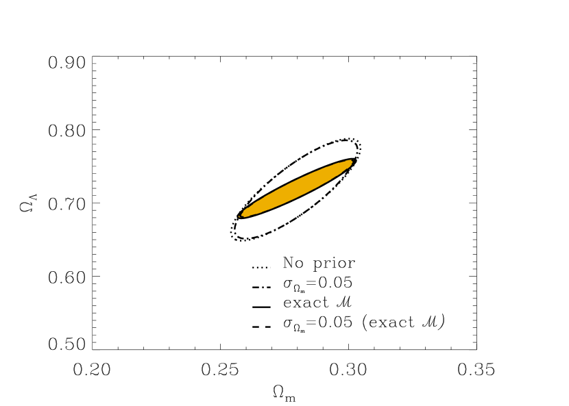
Figure 1: 68.3 % confidence regions for $(\Omega_{m},\Omega_{X})$ in the one-year SNAP scenario. The filled region assumes exact knowledge of ${\cal M}$ (solid and dashed lines approximately coincide). A full three-parameter fit with no prior knowledge of ${\cal M}$ is assumed for the two larger confidence regions: the region with a dotted line assumes no prior knowledge of $\Omega_{m}$, while the dash-dotted line assumes a prior knowledge with $\Omega_{m}$ Gaussian around the true value and $\sigma_{\Omega_{m}{\rm-prior}}=0.05$.

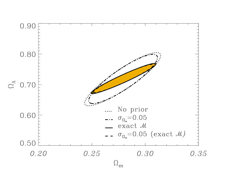
Figure 2: 68.3 % and 95% confidence regions for $(\Omega_{m},\Omega_{X})$ in the one-year SNAP scenario without the 100 events for which $z\in[1.2,1.7]$. The filled region (solid line) assumes exact knowledge of ${\cal M}$, and the dashed line within the filled region assumes also a prior knowledge with $\Omega_{m}$ Gaussian around the true value and $\sigma_{\Omega_{m}{\rm-prior}}=0.05$. A full three-parameter fit with no prior knowledge of ${\cal M}$ is assumed for the two larger confidence regions: the region with a dotted line assumes no prior knowledge of $\Omega_{m}$, while the dash-dotted line assumes a prior knowledge with $\Omega_{m}$ Gaussian around the true value and $\sigma_{\Omega_{m}{\rm-prior}}=0.05$.

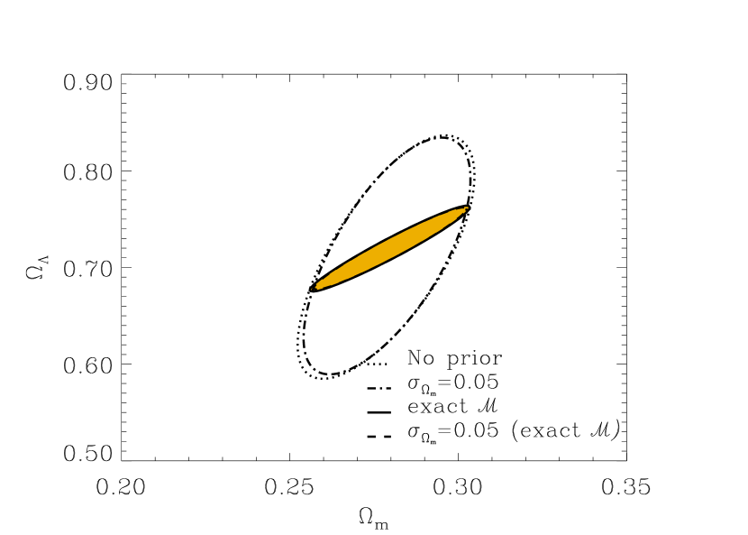
Figure 3: 68.3 % and 95 % confidence regions for $(\Omega_{m},\Omega_{X})$ in the one-year SNAP scenario with a constant rate per co-moving volume for $z\in[0,1.2]$, and the 100 $z\in[1.2,1.7]$ events uniformly distributed. The filled region assumes exact knowledge of ${\cal M}$ (solid and dashed lines approximately coincide). A full three-parameter fit with no prior knowledge of ${\cal M}$ is assumed for the two larger confidence regions: the region with a dotted line assumes no prior knowledge of $\Omega_{m}$, while the dash-dotted line assumes a prior knowledge with $\Omega_{m}$ Gaussian around the true value and $\sigma_{\Omega_{m}{\rm-prior}}=0.05$.

3.2 Confidence regions for $(\Omega_{m},w_{0})$ or $(\Omega_{X},w_{0})$

Next, we assume that the equation of state of the dark energy can be described by a constant $w=w_{0}$, so that $w_{1}=0$. Figures 4 – 6 show confidence regions for $(\Omega_{m},w_{0})$ or $(\Omega_{X},w_{0})$ under different assumptions that fix one parameter in the expression $\Omega_{\rm tot}=\Omega_{m}+\Omega_{X}$: figure 4 fixes the total energy density $\Omega_{\rm tot}=1$, which corresponds to a flat universe; figure 5 assumes that the density of the dark energy is known exactly, $\Omega_{X}=0.72$; figure 6 assumes that the energy density of ordinary matter is exactly known, $\Omega_{m}=0.28$. As before, we consider either exact knowledge of ${\cal M}$, or no prior knowledge. We also consider prior knowledge of either $\Omega_{m}$ or $\Omega_{\rm tot}$, with spread $\sigma_{\rm prior}=0.05$. It turns out that the (unrealistic) case where $\Omega_{X}$ is well-known gives the best determination of the other parameters under consideration, and that a good knowledge of $\Omega_{\rm tot}$ is preferred over a well-determined $\Omega_{m}$.

In figure 7, all three parameters $(\Omega_{m},\Omega_{X},w_{0})$ are allowed to vary, while both $\Omega_{m}$ and $\Omega_{\rm tot}$ are independently subject to Gaussian priors with $\sigma_{\Omega_{m}{\rm-prior}}=0.05$ and $\sigma_{\Omega_{\rm tot}{\rm-prior}}=0.05$. Comparing the case with exact ${\cal M}$ to the situation with no prior knowledge, it can be noted that the uncertainty of the latter mainly grows in $w_{0}$.

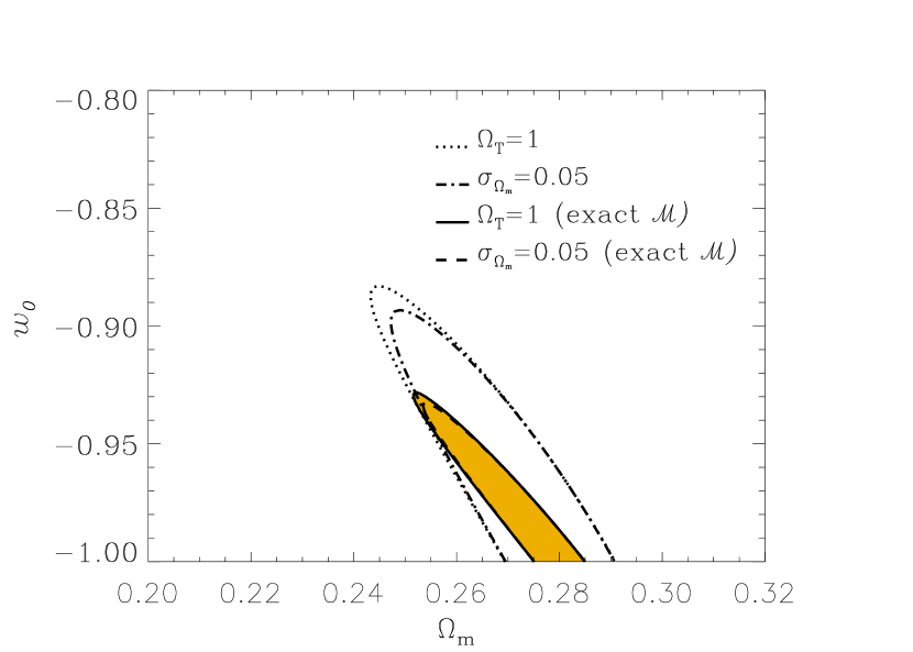
Figure 4: 68.3 % confidence regions for $(\Omega_{m},w_{0})$ in the one-year SNAP scenario with the flatness assumption $\Omega_{\rm tot}=1$. The filled region (solid line) assumes exact knowledge of ${\cal M}$, the dashed line within the filled region assumes also a prior knowledge with $\Omega_{m}$ Gaussian around the true value and $\sigma_{\Omega_{m}{\rm-prior}}=0.05$. The dotted and dash-dotted lines assume no prior knowledge of ${\cal M}$, without and with $\Omega_{m}$ prior, respectively.

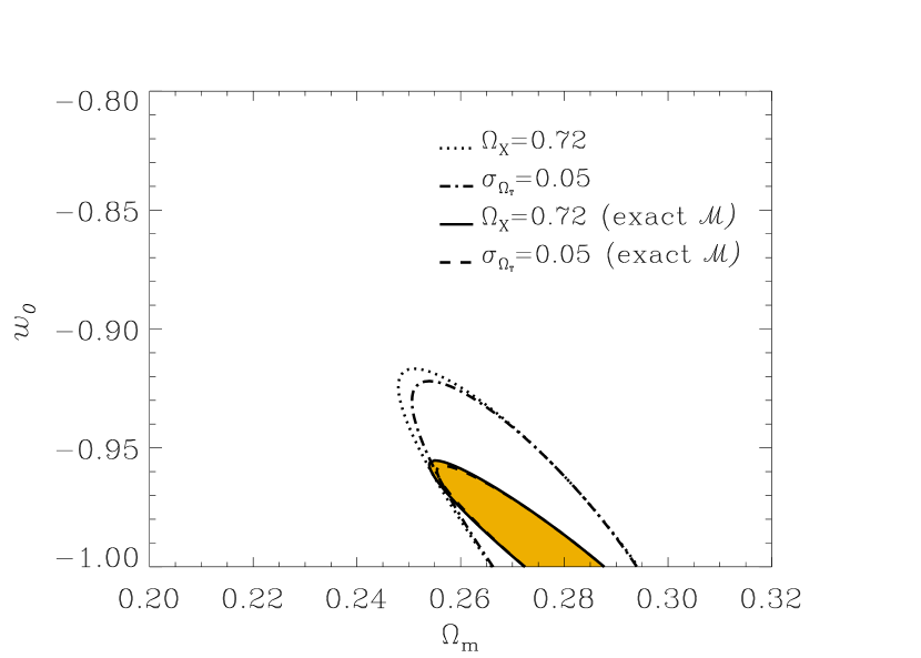
Figure 5: 68.3 % confidence regions for $(\Omega_{m},w_{0})$ in the one-year SNAP scenario assuming exact knowledge of $\Omega_{X}$, i.e., no prior knowledge on the geometry. The filled region (solid line) assumes exact knowledge of ${\cal M}$, the dashed line within the filled region assumes also a prior knowledge with $\Omega_{m}$ Gaussian around the true value and $\sigma_{\Omega_{m}{\rm-prior}}=0.05$. The dotted and dash-dotted lines assume no prior knowledge of ${\cal M}$, without and with $\Omega_{m}$ prior, respectively.

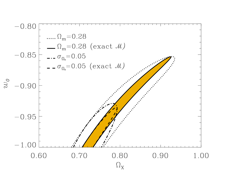
Figure 6: 68.3 % confidence regions for $(\Omega_{X},w_{0})$ in the one-year SNAP scenario assuming exact knowledge of $\Omega_{m}$. The filled region (solid line) assumes exact knowledge of ${\cal M}$, the dashed line within the filled region assumes also a prior knowledge with $\Omega_{\rm tot}$ Gaussian around the true value and $\sigma_{\Omega_{\rm tot}{\rm-prior}}=0.05$. The dotted and dash-dotted lines assume no prior knowledge of ${\cal M}$, without and with $\Omega_{\rm tot}$ prior, respectively.

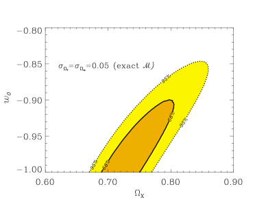
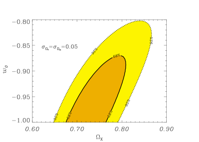
Figure 7: 68.3 % and 95 % confidence regions for $(\Omega_{X},w_{0})$ in the one-year SNAP scenario assuming prior knowledge with $\Omega_{m}$ and $\Omega_{\rm tot}$ independently Gaussian around their true values and $\sigma_{\Omega_{m}{\rm-prior}}=0.05=\sigma_{\Omega_{\rm tot}{\rm-prior}}$. The first figure assumes exact knowledge of ${\cal M}$, while the second assumes no prior knowledge of ${\cal M}$.

3.3 Confidence regions for $(w_{0},w_{1})$

Recently, Maor et al. (maor (2001); MBS) considered the problem of determining the equation of state of the dark energy using supernova measurements. In particular, they investigated an idealised experiment with thousands of supernovae in the redshift range $z\in[0,2]$, divided into 50 bins. The relative precision of the luminosity-distance $d_{L}$ was taken to be 0.6 % per bin, which corresponds to a magnitude precision $\sigma_{i}=0.006\times 5/\ln(10)\approx 0.0130$ for each bin. The equation of state is taken to be linear, $w(z)=w_{0}+w_{1}\,z$. Confidence regions for $(w_{0},w_{1})$ were determined, using the cosmology $\@vec{\theta}_{\rm true}=(0.3,0.7,-0.7,0)$. The log-likelihood was determined both for an exact $\Omega_{m}$, and with $\Omega_{m}$ integrated over $\Omega_{m,{\rm true}}\pm 0.1$.

Figure 8 shows our calculation of the confidence regions for this scenario. This figure should be compared with figure 2 of MBS. (Since MBS present one- and two-sigma contours, rather than the 68.3 % and 95 % confidence regions, we have included both cases to facilitate comparison.) There is a considerable discrepancy between these figures and MBS.

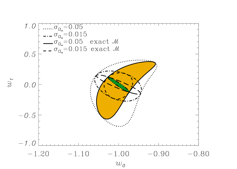
Figure 13: 68.3 % confidence regions for $(w_{0},w_{1})$ in the three-year SNAP scenario. The elongated ellipses correspond to the assumption of exact knowledge of $\Omega_{m}$: the dash-dot-dot-dotted line is with exact ${\cal M}$ and the long-dashed line corresponds to no knowledge of ${\cal M}$. The larger, non-elliptic regions assume Gaussian prior knowledge of $\Omega_{m}$: the dotted line is with $\sigma_{{\Omega_{m}}{\rm-prior}}=0.05$, while the dash-dotted line is with $\sigma_{\Omega_{m}{\rm-prior}}=0.015$. The solid and short-dashed lines assume exact knowledge of ${\cal M}$ with the same $\Omega_{m}$ priors as above.

In conclusion, it seems to us that this scenario enables a better constraining of $(w_{0},w_{1})$ than was previously anticipated by MBS. However, the scenario assumes that more than 6000 supernovae uniformly distributed over a rather optimistic redshift range are observed. Consequently, in this section, we calculate $(w_{0},w_{1})$ confidence regions for the cosmology of MBS, using the weaker precision and a smaller redshift range assumed in the SNAP proposal (snap (2000)), see figure 12 below. However, we focus our attention on the fiducial cosmology of SNAP: $\@vec{\theta}_{\rm true}=(0.28,0.72,-1,0)$ (see figures 9 – 11 and 13).

We consider the ability to determine the equation of state of the dark energy to linear order, $w(z)=w_{0}+w_{1}\,z$. We will assume flatness, $\Omega_{\rm tot}=1$, and impose some prior knowledge of $\Omega_{m}$. Figure 9 shows confidence regions for various assumptions regarding ${\cal M}$ and $\Omega_{m}$. We mainly consider a Gaussian prior with $\sigma_{\Omega_{m}{\rm-prior}}=0.05$. The uniform prior with $\Omega_{m}\in\Omega_{m,{\rm true}}\pm 0.1$ is considered in the case of exact knowledge of ${\cal M}$, since this is the situation considered by MBS. In figure 10, the few high-$z$ supernovae have been excluded. When ${\cal M}$ is exactly known, these are not so important in determining $(w_{0},w_{1})$ as they are for $(\Omega_{m},\Omega_{X})$, basically because $\Omega_{X}$ becomes less significant with increasing redshift. However, note that the high-$z$ events make some difference when ${\cal M}$ is poorly known. Figure 11 shows the situation when the supernovae at $z\in[0,1.2]$ are distributed according to a constant rate per co-moving volume element. As can be expected, uncertainties are not affected when ${\cal M}$ is considered to be exactly known, but degrade considerably with no prior information of ${\cal M}$. Figure 12 considers the same scenario as in figure 9 as regards precision and priors for $\Omega_{m}$, but uses the fiducial cosmology of MBS.

With the priors for $\Omega_{m}$ assumed in figures 9 – 12, the equation-of-state parameters are rather poorly constrained by one year of SNAP data, especially when ${\cal M}$ is left unspecified. In order to see what SNAP can achieve over its expected three years of operation, we calculate the confidence regions for thrice as many supernovae. Priors for $\Omega_{m}$ are Gaussian with $\sigma_{\Omega_{m}{\rm-prior}}=0.05$ as before, and we also consider $\sigma_{\Omega_{m}{\rm-prior}}=0.015$. The latter is consistent with the estimated precision of a hypothetical ground-based $10^{\circ}\times 10^{\circ}$ weak-lensing survey (van Waerbeke et al. waerbeke (1999)). (As discussed in this reference there is a weak dependence of $\Omega_{X}$ in these estimates of $\Omega_{m}$. We will not pursue this further here.) Uncertainties when $\Omega_{m}$ is exactly known (elliptic contours) improve the expected factor $1/\sqrt{3}$ as compared with the one-year scenario (compare with figure 9). For an $\Omega_{m}$ prior with $\sigma_{\Omega_{m}{\rm-prior}}=0.05$, confidence regions still span considerable parts of the parameter space. However, with the sharper prior, uncertainties in $w_{0}$ and $w_{1}$ go down to $w_{0}=-1\pm 0.02$, $w_{1}=0^{+0.13}_{-0.15}$ with an exact ${\cal M}$, and are still reasonable when imposing no prior knowledge of ${\cal M}$: $w_{0}=-1\pm 0.04$, $w_{1}=0^{+0.15}_{-0.17}$. Thus, it seems to us that three years of SNAP data backed up with independent high-precision observations of $\Omega_{m}$ can constrain the nature of the dark energy quite well. Note that in the above calculations we implicitly assume that the universe is known to be flat with high accuracy, since we have imposed $\Omega_{\rm tot}=1$.

Next, we turn our attention to the impact of different redshift distributions of supernovae on the confidence region in the ($w_{0},w_{1}$) parameter space. The interval $z\in[0,2]$ is divided into 8 subsets containing 500 supernovae each uniformly distributed in redshift as: $z_{1}=[0,0.25]$, $z_{2}=[0.25,0.5]$, $z_{3}=[0.5,0.75]$,.., $z_{8}=[1.75,2.0]$. We then compose 4 different experimental situations where in each case 2000 supernovae are measured ($\Delta m$ = 0.16 mag /SN) sampling events from $[z_{1},z_{2},z_{3},z_{4}]$, $[z_{1},z_{2},z_{7},z_{8}]$, $[z_{2},z_{4},z_{6},z_{8}]$ and $[z_{5},z_{6},z_{7},z_{8}]$, as shown in figure 14 for the case $\@vec{\theta}=(0.3,0.7,-1,0)$ where the mass energy density is given a uniform prior with $\Delta\Omega_{m}=0.1$. Clearly, a wide range of supernova redshifts is more advantageous than only data above or below $z=1$.

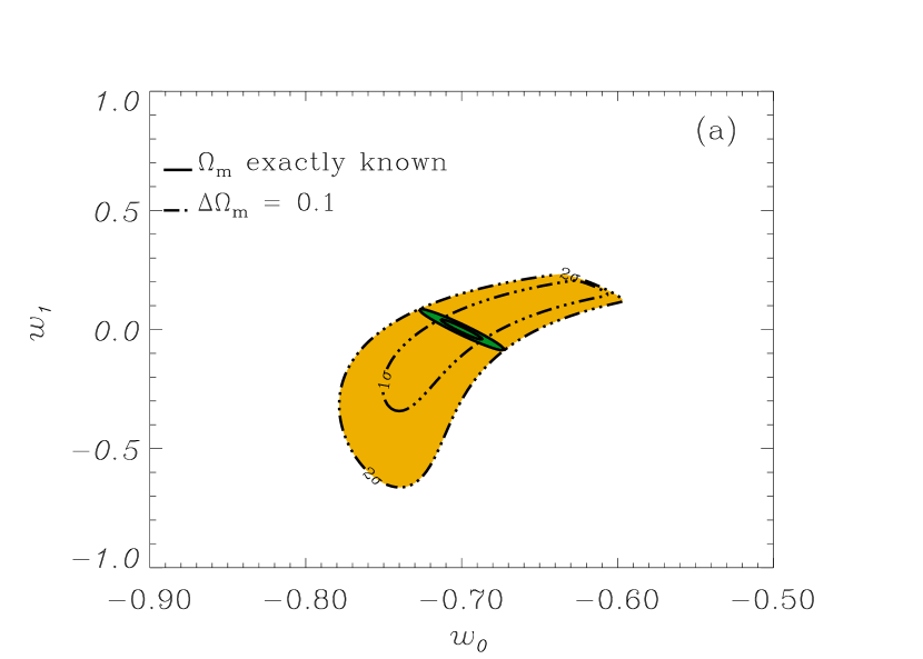
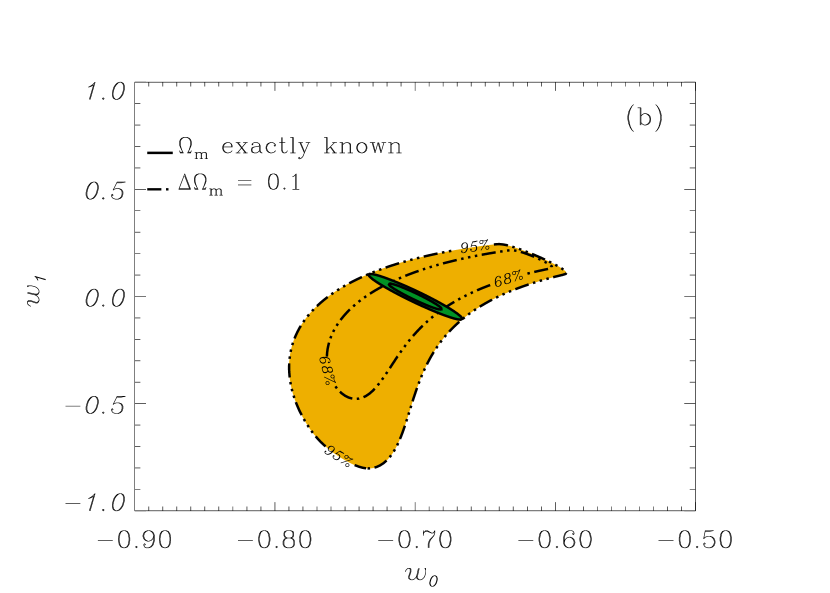
Figure 8: (a) 1$\sigma$ and 2$\sigma$ confidence regions for $(w_{0},w_{1})$ using the scenario of Maor et al. (maor (2001)). The elongated ellipses correspond to the assumption of exact knowledge of $\Omega_{m}$, while the larger, non-elliptic regions assume the prior knowledge that $\Omega_{m}$ is confined to the interval $\Omega_{m,{\rm true}}\pm 0.1$. Exact knowledge of ${\cal M}$ is assumed. (b) 68.3 % and 95 % confidence regions for the same cosmology.

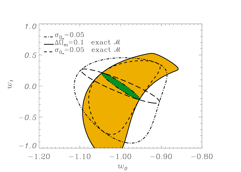
Figure 9: 68.3 % confidence regions for $(w_{0},w_{1})$ in the one-year SNAP scenario. The elongated ellipses correspond to the assumption of exact knowledge of $\Omega_{m}$: the dash-dot-dot-dotted line is with exact ${\cal M}$ and the long-dashed line corresponds to no knowledge of ${\cal M}$. The larger, non-elliptic regions assume prior knowledge of $\Omega_{m}$: the dash-dotted line assumes that $\Omega_{m}$ is known with a Gaussian prior for which $\sigma_{\Omega_{m}{\rm-prior}}=0.05$; the short-dashed line assumes the same prior and exact knowledge of ${\cal M}$; finally, the solid line is with $\Omega_{m}$ confined to the interval $\Omega_{m}\pm 0.1$ and exact knowledge of ${\cal M}$.

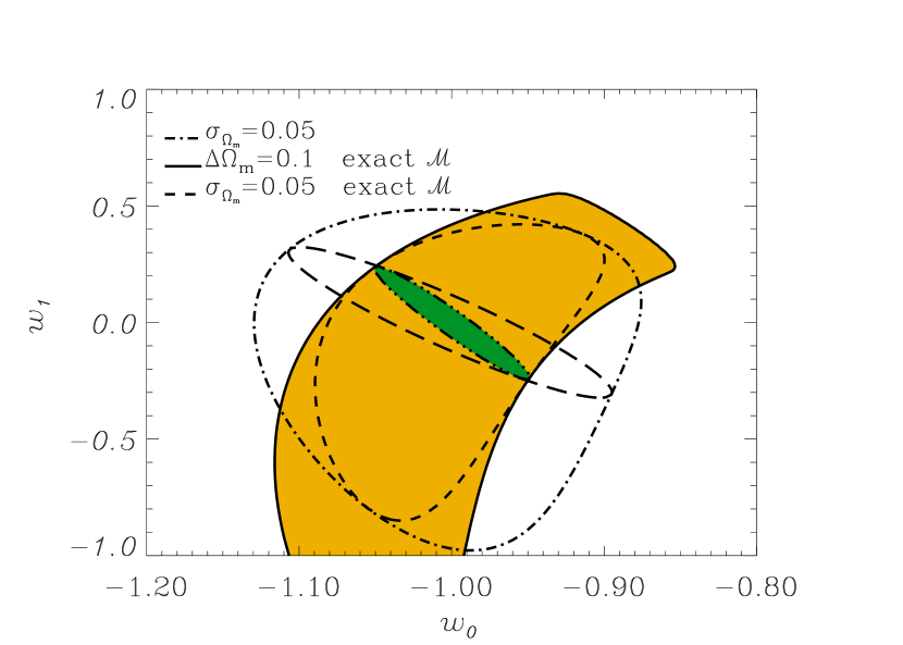
Figure 10: 68.3 % confidence regions for $(w_{0},w_{1})$ in the one-year SNAP scenario without the 100 events for which $z\in[1.2,1.7]$. The elongated ellipses correspond to the assumption of exact knowledge of $\Omega_{m}$: the dash-dot-dot-dotted line is with exact ${\cal M}$ and the long-dashed line corresponds to no knowledge of ${\cal M}$. The larger, non-elliptic regions assume prior knowledge of $\Omega_{m}$: the dash-dotted line assumes that $\Omega_{m}$ is known with a Gaussian prior for which $\sigma_{\Omega_{m}{\rm-prior}}=0.05$; the short-dashed line assumes the same prior and exact knowledge of ${\cal M}$; finally, the solid line is with $\Omega_{m}$ confined to the interval $\Omega_{m}\pm 0.1$ and exact knowledge of ${\cal M}$.

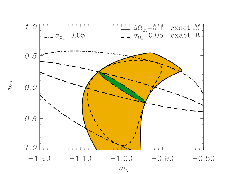
Figure 11: 68.3 % confidence regions for $(w_{0},w_{1})$ in the one-year SNAP scenario with a constant rate per co-moving volume for $z\in[0,1.2]$, and the 100 $z\in[1.2,1.7]$ events uniformly distributed. The elongated ellipses correspond to the assumption of exact knowledge of $\Omega_{m}$: the dash-dot-dot-dotted line is with exact ${\cal M}$ and the long-dashed line corresponds to no knowledge of ${\cal M}$. The larger, non-elliptic regions assume prior knowledge of $\Omega_{m}$: the dash-dotted line assumes that $\Omega_{m}$ is known with a Gaussian prior for which $\sigma_{\Omega_{m}{\rm-prior}}=0.05$; the short-dashed line assumes the same prior and exact knowledge of ${\cal M}$; finally, the solid line is with $\Omega_{m}$ confined to the interval $\Omega_{m}\pm 0.1$ and exact knowledge of ${\cal M}$.

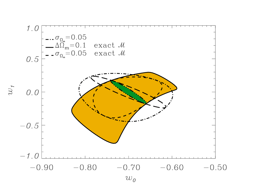
Figure 12: 68.3 % confidence regions for $(w_{0},w_{1})$ assuming the precision of the one-year SNAP scenario, but the cosmology of Maor et al. (maor (2001)). The elongated ellipses correspond to the assumption of exact knowledge of $\Omega_{m}$: the dash-dot-dot-dotted line is with exact ${\cal M}$ and the long-dashed line corresponds to no knowledge of ${\cal M}$. The larger, non-elliptic regions assume prior knowledge of $\Omega_{m}$: the dash-dotted line assumes that $\Omega_{m}$ is known with a Gaussian prior for which $\sigma_{\Omega_{m}{\rm-prior}}=0.05$; the short-dashed line assumes the same prior and exact knowledge of ${\cal M}$; finally, the solid line is with $\Omega_{m}$ confined to the interval $\Omega_{m}\pm 0.1$ and exact knowledge of ${\cal M}$.

Figure 14: 68.3 % confidence regions for $(w_{0},w_{1})$ with 2000 supernovae. The importance of wide redshift coverage is demonstrated by simulating four different synthetic experiments, all consisting of 2000 SNe: 1234 includes SNe uniformly distributed in $z\in[0,1]$, experiment 5678 has only SNe uniformly distributed in $z\in[1,2]$, experiment 1278 has supernovae in uniformly distributed in two bins, $z\in[0,0.5]$ and $z\in[1.5,2]$. Finally, experiment 2468 includes four bins: $z\in[0.25,0.5]$, $z\in[0.75,1]$, $z\in[1.25,1.5]$ and $z\in[1.75,2]$. Clearly, the two experiments with the widest redshift coverage provide the best constraints.

4 Effect of adding a small sample of supernovae

To further illustrate the importance of a small number of high-redshift events, we have performed Fisher analyses (see appendix A.2 and (Astier astier (2001))) to investigate the effect of adding 100 supernovae to a large initial sample at lower redshift. We do this for initially 2000 supernovae uniformly distributed at $z\in[0,1.2]$. To emphasize the importance of events at very low redshift, we do the same exercise for initially 2000 supernovae uniformly distributed at $z\in[0.2,1.2]$. Since the effects depend significantly on the underlying cosmological model, we investigate three models: the fiducial model of the SNAP proposal (snap (2000)): $\@vec{\theta}_{\rm true}=(0.28,0.72,-1,0)$, a quintessence model derived from supergravity considerations (Brax & Martin brax (1999)) $\@vec{\theta}_{\rm true}=(0.28,0.72,-0.8,0.3)$, and the model used by Maor et al. (maor (2001)) $\@vec{\theta}_{\rm true}=(0.3,0.7,-0.7,0)$.

Figures 15 and 16 show the effect on the errors of $\Omega_{m}$ and $\Omega_{X}$ when adding 100 supernovae to the samples outlined above. As expected, high redshifts pay off when determining $\Omega_{m}$ and $\Omega_{X}$, but in case the knowledge of ${\cal M}$ is poor, it is also important to fill the low-redshift region. Note that the curves for exact ${\cal M}$ have two minima ($z_{\rm max}$ and one intermediate redshift), while those where ${\cal M}$ is unknown have three ($z_{\rm min}$, $z_{\rm max}$ and one intermediate redshift). This is only a manifestation of the fact that the optimum redshift distribution with $n$ parameters consists of $n$ $\delta$ functions (Astier astier (2001)). (When priors are imposed this may no longer be the case.) Furthermore, for each curve there are two values of the redshift where it is totally ineffectual to add more events.

Figures 17 – 20 assume a flat universe, and consider $(w_{0},w_{1})$ for the same initial distributions. In figures 17 and 18 $\Omega_{m}$ is exactly known, while in figures 19 and 20 a Gaussian prior with $\sigma_{\Omega_{m}{\rm-prior}}=0.05$ is imposed. The pay-off with high-redshift events is not as great as when determining $(\Omega_{m},\Omega_{X})$. In particular, note that the cosmological-constant model is the worst case of the scenarios we have considered.

\psfrag{labellabellabel1}{\tiny{$\cal{M}$ unknown}}\psfrag{labellabellabel2}{\tiny{$\cal{M}$ unknown}}\psfrag{labellabellabel3}{\tiny{$\cal{M}$ unknown}}\psfrag{labellabellabel4}{\tiny{$\cal{M}$ unknown}}\psfrag{wzeroMscriptunknown}{\tiny{$\cal{M}$ unknown}}\psfrag{woneMscriptunknown}{\tiny{$\cal{M}$ unknown}}\psfrag{wzeroomegamGaussian}{\tiny{$\Omega_{m}$ Gaussian}}\psfrag{woneomegamGaussian}{\tiny{$\Omega_{m}$ Gaussian}}\psfrag{wzeroomegamGaussianMscript unknown}{\tiny{$\Omega_{m}$ Gaussian, $\cal{M}$ unk.}}\psfrag{wzeroomegamGaussianMscriptunknown}{\tiny{$\Omega_{m}$ Gaussian, $\cal{M}$ unk.}}\psfrag{woneomegamGaussianMscriptunknown}{\tiny{$\Omega_{m}$ Gaussian, $\cal{M}$ unk.}}\psfrag{omegam}{\tiny{}}\psfrag{omegax}{\tiny{}}\psfrag{wzero}{\tiny{}}\psfrag{wone}{\tiny{}}\includegraphics[width=433.62pt]{add01-06_ag.eps}

Figure 15: The effect on $\sigma_{\Omega_{m}}$ and $\sigma_{\Omega_{X}}$ when 100 supernovae are added at a specific redshift $z\in[0,2]$. The original sample consists of 2000 supernovae uniformly distributed over $z\in[0,1.2]$. Solid lines correspond to the SNAP fiducial model $(\Omega_{m},\Omega_{X},w_{0},w_{1})=(0.28,0.72,-1,0)$, dashed lines correspond to $(\Omega_{m},\Omega_{X},w_{0},w_{1})=(0.28,0.72,-0.8,0.3)$, and dotted lines correspond to $(\Omega_{m},\Omega_{X},w_{0},w_{1})=(0.3,0.7,-0.7,0)$.

\psfrag{labellabellabel1}{\tiny{$\cal{M}$ unknown}}\psfrag{labellabellabel2}{\tiny{$\cal{M}$ unknown}}\psfrag{labellabellabel3}{\tiny{$\cal{M}$ unknown}}\psfrag{labellabellabel4}{\tiny{$\cal{M}$ unknown}}\psfrag{wzeroMscriptunknown}{\tiny{$\cal{M}$ unknown}}\psfrag{woneMscriptunknown}{\tiny{$\cal{M}$ unknown}}\psfrag{wzeroomegamGaussian}{\tiny{$\Omega_{m}$ Gaussian}}\psfrag{woneomegamGaussian}{\tiny{$\Omega_{m}$ Gaussian}}\psfrag{wzeroomegamGaussianMscript unknown}{\tiny{$\Omega_{m}$ Gaussian, $\cal{M}$ unk.}}\psfrag{wzeroomegamGaussianMscriptunknown}{\tiny{$\Omega_{m}$ Gaussian, $\cal{M}$ unk.}}\psfrag{woneomegamGaussianMscriptunknown}{\tiny{$\Omega_{m}$ Gaussian, $\cal{M}$ unk.}}\psfrag{omegam}{\tiny{}}\psfrag{omegax}{\tiny{}}\psfrag{wzero}{\tiny{}}\psfrag{wone}{\tiny{}}\includegraphics[width=433.62pt]{add07-12_ag}

Figure 16: The effect on $\sigma_{\Omega_{m}}$ and $\sigma_{\Omega_{X}}$ when 100 supernovae are added at a specific redshift $z\in[0,2]$. The original sample consists of 2000 supernovae uniformly distributed over $z\in[0.2,1.2]$. Solid lines correspond to the SNAP fiducial model $(\Omega_{m},\Omega_{X},w_{0},w_{1})=(0.28,0.72,-1,0)$, dashed lines correspond to $(\Omega_{m},\Omega_{X},w_{0},w_{1})=(0.28,0.72,-0.8,0.3)$, and dotted lines correspond to $(\Omega_{m},\Omega_{X},w_{0},w_{1})=(0.3,0.7,-0.7,0)$.

\psfrag{labellabellabel1}{\tiny{$\cal{M}$ unknown}}\psfrag{labellabellabel2}{\tiny{$\cal{M}$ unknown}}\psfrag{labellabellabel3}{\tiny{$\cal{M}$ unknown}}\psfrag{labellabellabel4}{\tiny{$\cal{M}$ unknown}}\psfrag{wzeroMscriptunknown}{\tiny{$\cal{M}$ unknown}}\psfrag{woneMscriptunknown}{\tiny{$\cal{M}$ unknown}}\psfrag{wzeroomegamGaussian}{\tiny{$\Omega_{m}$ Gaussian}}\psfrag{woneomegamGaussian}{\tiny{$\Omega_{m}$ Gaussian}}\psfrag{wzeroomegamGaussianMscript unknown}{\tiny{$\Omega_{m}$ Gaussian, $\cal{M}$ unk.}}\psfrag{wzeroomegamGaussianMscriptunknown}{\tiny{$\Omega_{m}$ Gaussian, $\cal{M}$ unk.}}\psfrag{woneomegamGaussianMscriptunknown}{\tiny{$\Omega_{m}$ Gaussian, $\cal{M}$ unk.}}\psfrag{omegam}{\tiny{}}\psfrag{omegax}{\tiny{}}\psfrag{wzero}{\tiny{}}\psfrag{wone}{\tiny{}}\includegraphics[width=433.62pt]{add13-18_ag}

Figure 17: The effect on $\sigma_{w_{0}}$ and $\sigma_{w_{1}}$ when 100 supernovae are added at a specific redshift $z\in[0,2]$. The original sample consists of 2000 supernovae uniformly distributed over $z\in[0,1.2]$. $\Omega_{m}$ and $\Omega_{X}$ are assumed to be exactly known. Solid lines correspond to the SNAP fiducial model $(\Omega_{m},\Omega_{X},w_{0},w_{1})=(0.28,0.72,-1,0)$, dashed lines correspond to $(\Omega_{m},\Omega_{X},w_{0},w_{1})=(0.28,0.72,-0.8,0.3)$, and dotted lines correspond to $(\Omega_{m},\Omega_{X},w_{0},w_{1})=(0.3,0.7,-0.7,0)$.

\psfrag{labellabellabel1}{\tiny{$\cal{M}$ unknown}}\psfrag{labellabellabel2}{\tiny{$\cal{M}$ unknown}}\psfrag{labellabellabel3}{\tiny{$\cal{M}$ unknown}}\psfrag{labellabellabel4}{\tiny{$\cal{M}$ unknown}}\psfrag{wzeroMscriptunknown}{\tiny{$\cal{M}$ unknown}}\psfrag{woneMscriptunknown}{\tiny{$\cal{M}$ unknown}}\psfrag{wzeroomegamGaussian}{\tiny{$\Omega_{m}$ Gaussian}}\psfrag{woneomegamGaussian}{\tiny{$\Omega_{m}$ Gaussian}}\psfrag{wzeroomegamGaussianMscript unknown}{\tiny{$\Omega_{m}$ Gaussian, $\cal{M}$ unk.}}\psfrag{wzeroomegamGaussianMscriptunknown}{\tiny{$\Omega_{m}$ Gaussian, $\cal{M}$ unk.}}\psfrag{woneomegamGaussianMscriptunknown}{\tiny{$\Omega_{m}$ Gaussian, $\cal{M}$ unk.}}\psfrag{omegam}{\tiny{}}\psfrag{omegax}{\tiny{}}\psfrag{wzero}{\tiny{}}\psfrag{wone}{\tiny{}}\includegraphics[width=433.62pt]{add19-24_ag}

Figure 18: The effect on $\sigma_{w_{0}}$ and $\sigma_{w_{1}}$ when 100 supernovae are added at a specific redshift $z\in[0,2]$. The original sample consists of 2000 supernovae uniformly distributed over $z\in[0.2,1.2]$. $\Omega_{m}$ and $\Omega_{X}$ are assumed to be exactly known. Solid lines correspond to the SNAP fiducial model $(\Omega_{m},\Omega_{X},w_{0},w_{1})=(0.28,0.72,-1,0)$, dashed lines correspond to $(\Omega_{m},\Omega_{X},w_{0},w_{1})=(0.28,0.72,-0.8,0.3)$, and dotted lines correspond to $(\Omega_{m},\Omega_{X},w_{0},w_{1})=(0.3,0.7,-0.7,0)$.

\psfrag{labellabellabel1}{\tiny{$\cal{M}$ unknown}}\psfrag{labellabellabel2}{\tiny{$\cal{M}$ unknown}}\psfrag{labellabellabel3}{\tiny{$\cal{M}$ unknown}}\psfrag{labellabellabel4}{\tiny{$\cal{M}$ unknown}}\psfrag{wzeroMscriptunknown}{\tiny{$\cal{M}$ unknown}}\psfrag{woneMscriptunknown}{\tiny{$\cal{M}$ unknown}}\psfrag{wzeroomegamGaussian}{\tiny{$\Omega_{m}$ Gaussian}}\psfrag{woneomegamGaussian}{\tiny{$\Omega_{m}$ Gaussian}}\psfrag{wzeroomegamGaussianMscript unknown}{\tiny{$\Omega_{m}$ Gaussian, $\cal{M}$ unk.}}\psfrag{wzeroomegamGaussianMscriptunknown}{\tiny{$\Omega_{m}$ Gaussian, $\cal{M}$ unk.}}\psfrag{woneomegamGaussianMscriptunknown}{\tiny{$\Omega_{m}$ Gaussian, $\cal{M}$ unk.}}\psfrag{omegam}{\tiny{}}\psfrag{omegax}{\tiny{}}\psfrag{wzero}{\tiny{}}\psfrag{wone}{\tiny{}}\includegraphics[width=433.62pt]{add25-30_ag}

Figure 19: The effect on $\sigma_{w_{0}}$ and $\sigma_{w_{1}}$ when 100 supernovae are added at a specific redshift $z\in[0,2]$. The original sample consists of 2000 supernovae uniformly distributed over $z\in[0,1.2]$. $\Omega_{X}$ is assumed to be exactly known, while $\Omega_{m}$ is known within $\sigma_{\Omega_{m}{\rm-prior}}=0.05$. Solid lines correspond to the SNAP fiducial model $(\Omega_{m},\Omega_{X},w_{0},w_{1})=(0.28,0.72,-1,0)$, dashed lines correspond to $(\Omega_{m},\Omega_{X},w_{0},w_{1})=(0.28,0.72,-0.8,0.3)$, and dotted lines correspond to $(\Omega_{m},\Omega_{X},w_{0},w_{1})=(0.3,0.7,-0.7,0)$.

\psfrag{labellabellabel1}{\tiny{$\cal{M}$ unknown}}\psfrag{labellabellabel2}{\tiny{$\cal{M}$ unknown}}\psfrag{labellabellabel3}{\tiny{$\cal{M}$ unknown}}\psfrag{labellabellabel4}{\tiny{$\cal{M}$ unknown}}\psfrag{wzeroMscriptunknown}{\tiny{$\cal{M}$ unknown}}\psfrag{woneMscriptunknown}{\tiny{$\cal{M}$ unknown}}\psfrag{wzeroomegamGaussian}{\tiny{$\Omega_{m}$ Gaussian}}\psfrag{woneomegamGaussian}{\tiny{$\Omega_{m}$ Gaussian}}\psfrag{wzeroomegamGaussianMscript unknown}{\tiny{$\Omega_{m}$ Gaussian, $\cal{M}$ unk.}}\psfrag{wzeroomegamGaussianMscriptunknown}{\tiny{$\Omega_{m}$ Gaussian, $\cal{M}$ unk.}}\psfrag{woneomegamGaussianMscriptunknown}{\tiny{$\Omega_{m}$ Gaussian, $\cal{M}$ unk.}}\psfrag{omegam}{\tiny{}}\psfrag{omegax}{\tiny{}}\psfrag{wzero}{\tiny{}}\psfrag{wone}{\tiny{}}\includegraphics[width=433.62pt]{add31-36_ag}

Figure 20: Effect on $\sigma_{w_{0}}$ and $\sigma_{w_{1}}$ when 100 supernovae are added at a specific redshift $z\in[0,2]$. The original sample consists of 2000 supernovae uniformly distributed over $z\in[0.2,1.2]$. $\Omega_{X}$ is assumed to be exactly known, while $\Omega_{m}$ is known within $\sigma_{\Omega_{m}{\rm-prior}}=0.05$. Solid lines correspond to the SNAP fiducial model $(\Omega_{m},\Omega_{X},w_{0},w_{1})=(0.28,0.72,-1,0)$, dashed lines correspond to $(\Omega_{m},\Omega_{X},w_{0},w_{1})=(0.28,0.72,-0.8,0.3)$, and dotted lines correspond to $(\Omega_{m},\Omega_{X},w_{0},w_{1})=(0.3,0.7,-0.7,0)$.

5 Lensing bias

So far, the analysis has not taken into account any systematic errors in the magnitude measurements. However, there are several possible mechanisms that can give rise to redshift-dependent systematics: attenuation by “gray dust” in the intergalactic medium would cause distant sources to look fainter than they really are, and evolutionary effects $M=M(z)$ of the absolute magnitude of supernovae Ia are currently not well-known. Furthermore, the effects of gravitational lensing increase with redshift, and the corresponding magnitude distributions become markedly non-Gaussian for sources at high redshift.

We have investigated the effects from gravitational lensing by using the method of Holz & Wald (hw (1998)), see further (Bergström et al. lens (2000)). The inhomogeneities are modelled as halos with the density profile as proposed by Navarro et al. (nfw (1997)). We consider the cosmology examined by Maor et al. (maor (2001)), $\@vec{\theta}=(0.3,0.7,-0.7,0)$, and use the redshift distribution given by table 7.2 in the SNAP proposal (snap (2000)). Note that this distribution is different from the ones used previously. Figure 21 shows the lensing effects in the $(w_{0},w_{1})$ space. In this particular parameter space the lensing effects are negligible compared with the intrinsic uncertainty in the $(w_{0},w_{1})$ measurements. However, sizable effects have to be considered for the $(\Omega_{m},\Omega_{X})$ parameter space, especially if $\Omega_{m}$ contains a significant fraction of point-like objects, such as MACHOs (Amanullah et al. ramme (2001)).

\psfrag{labellabellabel1}{\tiny{$\cal{M}$ unknown}}\psfrag{labellabellabel2}{\tiny{$\cal{M}$ unknown}}\psfrag{labellabellabel3}{\tiny{$\cal{M}$ unknown}}\psfrag{labellabellabel4}{\tiny{$\cal{M}$ unknown}}\psfrag{wzeroMscriptunknown}{\tiny{$\cal{M}$ unknown}}\psfrag{woneMscriptunknown}{\tiny{$\cal{M}$ unknown}}\psfrag{wzeroomegamGaussian}{\tiny{$\Omega_{m}$ Gaussian}}\psfrag{woneomegamGaussian}{\tiny{$\Omega_{m}$ Gaussian}}\psfrag{wzeroomegamGaussianMscript unknown}{\tiny{$\Omega_{m}$ Gaussian, $\cal{M}$ unk.}}\psfrag{wzeroomegamGaussianMscriptunknown}{\tiny{$\Omega_{m}$ Gaussian, $\cal{M}$ unk.}}\psfrag{woneomegamGaussianMscriptunknown}{\tiny{$\Omega_{m}$ Gaussian, $\cal{M}$ unk.}}\psfrag{omegam}{\tiny{}}\psfrag{omegax}{\tiny{}}\psfrag{wzero}{\tiny{}}\psfrag{wone}{\tiny{}}\includegraphics[width=433.62pt]{maor-lins_idl}

Figure 21: 68.3 % confidence region for $(w_{0},w_{1})$ for one year of SNAP for the cosmology in maor (2001), central values at $w_{0}=-0.7$ and $w_{1}=0$ (solid line). The dashed curve incorporates the bias effects form gravitational lensing magnification.

6 Discussion

This analysis stresses the importance of combining independent estimations of the cosmological parameters in order to probe the nature of the dark energy as accurately as possible. For instance, we conclude that a mission for observing supernovae over a large redshift range, such as the SuperNova/Acceleration Probe (SNAP), can give reasonable constraints on the equation of state of the dark energy, provided three years of observational data and good prior knowledge of the geometry and matter density of the universe. To exemplify, we expect SNAP to be able to determine the parameters in a linear equation of state $w(z)=w_{0}+w_{1}\,z$ to within $\pm 0.04$ for $w_{0}$ and ${}^{+0.15}_{-0.17}$ for $w_{1}$ (one-parameter one-sigma levels), assuming a flat universe, the matter energy density known with $\sigma_{\Omega_{m}{\rm-prior}}\pm 0.015$, but no prior knowledge imposed on the intercept ${\cal M}$. These estimates assume that the overall error budget is not dominated by systematic uncertainties. With one year of SNAP data, $w_{0}$ could be within 10 % provided that the equation of state is assumed to be constant, $w=w_{0}$.

It is important to realise that data at low as well as high redshift is required for an optimal parameter estimation. Events at very low redshift help to fix the intercept ${\cal M}$, while a wide range of redshifts is needed to break the degeneracy in the luminosity distance between different cosmologies.

Appendix A Methodology

We determine two-dimensional confidence regions for subsets $(\theta_{1},\theta_{2})\in\@vec{\theta}$ of the parameters $\@vec{\theta}=(\Omega_{m},\Omega_{X},w_{0},w_{1})$, while imposing various conditions on the remaining parameters. To this end, we construct log-likelihood functions $\chi^{2}$ based on hypothetical magnitude measurements at various redshifts:

$$\chi^{2}=\sum_{i=1}^{n}\frac{\left[m(\@vec{\theta},{\cal M},z_{i})-m(\@vec{\theta}_{\rm true},{\cal M}_{\rm true},z_{i})\right]^{2}}{\sigma_{i}^{2}},$$ (12)

where $m(\@vec{\theta},{\cal M},z)$ is the apparent magnitude of a supernova at redshift $z$ in the cosmology $\@vec{\theta}$ (see section 2 above), and the sum is over bins at different redshifts. The subscript _true denotes actual cosmological parameter values. The precision $\sigma_{i}$ of each bin is given by the individual measurement precision $\Delta m$ and the number of supernovae $n_{i}$ in the bin by $\sigma_{i}=\Delta m/\sqrt{n_{i}}$.

Often, we will impose prior knowledge of $\Omega_{m}$ and/or $\Omega_{\rm tot}=\Omega_{m}+\Omega_{X}$. When the parameter $\theta$ of which we have prior knowledge is one of the two we are interested in, $\theta\in(\theta_{1},\theta_{2})$, a Gaussian prior knowledge of $\theta$ with spread $\sigma_{\theta{\rm-prior}}$ is easily added:

$$\chi^{2}=\chi^{2}_{0}+\frac{(\theta-\theta_{\rm true})^{2}}{\sigma_{\theta{\rm-prior}}^{2}},$$ (13)

where $\chi^{2}_{0}$ denotes the $\chi^{2}$ obtained without imposing the prior knowledge of $\theta$. In case $\theta\notin(\theta_{1},\theta_{2})$, we have to integrate out $\theta$ from the likelihood $L=\exp(-\frac{1}{2}\chi^{2})$ with some prior $\pi(\theta)$ to obtain $\chi^{2}_{\theta{\rm-int}}$:

$$\chi^{2}_{\theta{\rm-int}}=-2\ln\left[\int_{-\infty}^{\infty}\,d\theta\exp\left(-\frac{1}{2}\chi^{2}\right)\,\pi(\theta)\right].$$ (14)

Note that the form of (14) implies that a constant additive to $\chi^{2}$ simply adds to the integrated log-likelihood $\chi^{2}_{\theta{\rm-int}}$:

$$-2\ln\left[\int\,d\theta\exp\left(-\frac{1}{2}(\chi^{2}+A)\right)\pi(\theta)\right]=\chi^{2}_{\theta{\rm-int}}+A,$$ (15)

and that $\chi^{2}_{\theta{\rm-int}}-\chi^{2}_{\theta{\rm-int,min}}$ is unaffected by any such constant. Consequently, we can equally well define

$$\chi^{2}_{\theta{\rm-int}}\equiv-2\ln\left[\int\,d\theta\exp\left(-\frac{1}{2}(\chi^{2}-\chi^{2}_{\rm min})\right)\,\pi(\theta)\right].$$ (16)

We will use Gaussian priors

$$\pi(\theta)=\frac{1}{\sqrt{2\pi\sigma_{\theta{\rm-prior}}^{2}}}\exp\left[-\frac{1}{2\sigma_{\theta{\rm-prior}}^{2}}(\theta-\theta_{\rm true})^{2}\right],$$ (17)

but also uniform priors $\pi(\theta)=1$ with $\theta$ confined to an interval $\theta\in\theta_{\rm true}\pm\Delta\theta$. A special case is the treatment of the intercept ${\cal M}$, for which we assume both exact knowledge, but also no prior knowledge at all. Hence, integrating ${\cal M}$ over all possible values ${\cal M}\in(-\infty,\infty)$, we obtain an analytic expression for $\chi^{2}_{{\cal M}{\rm-int}}$, see appendix A.1.

Given the appropriate $\chi^{2}$ function, 68.3 % and 95 % confidence regions are defined by the conventional two-parameter $\chi^{2}$ levels 2.30 and 5.99, respectively. Similarly, one-parameter one- and two-sigma levels correspond to $\chi^{2}=$ 1 and 4, respectively. In some cases we need to calculate $\chi^{2}$ for three parameters, and subsequently project onto the $(\theta_{1},\theta_{2})$ plane of interest. This can be done by setting $\chi^{2}={\rm min}\,[\chi^{2}(\cdots,\theta_{3})]$, where the minimisation of $\chi^{2}$ is performed with respect to variation of $\theta_{3}$. Confidence regions for $(\theta_{1},\theta_{2})$ can then be determined using the usual two-parameter $\chi^{2}$ levels.

A.1 Integration over the intercept ${\cal M}$

When the intercept is assumed to be exactly known ${\cal M}={\cal M}_{\rm true}$, it will cancel in the expression for $\chi^{2}$, so that we obtain the log-likelihood $\hat{\chi}^{2}$ as

$$\hat{\chi}^{2} \equiv \sum_{i=1}^{n}\frac{\Delta^{2}}{\sigma_{i}^{2}},$$ (18)

$$\Delta = 5\log_{10}\left[d^{\prime}_{L}(\@vec{\theta},z_{i})\right]-5\log_{10}\left[d^{\prime}_{L}(\@vec{\theta}_{\rm true},z_{i})\right].$$ (19)

Note that $\hat{\chi}^{2}_{\rm min}=\hat{\chi}^{2}(\@vec{\theta}_{\rm true})=0$ by construction.

If no prior knowledge of ${\cal M}$ at all is assumed, we can integrate the general $\chi^{2}$ function (12) over ${\cal M}\in(-\infty,\infty)$ to obtain an analytic expression for $\tilde{\chi}^{2}\equiv\chi^{2}_{{\cal M}{\rm-int}}$:

$$\tilde{\chi}^{2} = -2\ln\left[\int_{-\infty}^{\infty}\,d{\cal M}\exp\left(-\frac{1}{2}\chi^{2}\right)\right]$$ (20)

$$= \hat{\chi}^{2}-\frac{B^{2}}{C}+\ln\left(\frac{C}{2\pi}\right),$$ (21)

$$B = \sum_{i=1}^{n}\frac{\Delta}{\sigma_{i}^{2}},$$ (22)

$$C = \sum_{i=1}^{n}\frac{1}{\sigma_{i}^{2}}.$$ (23)

Note that this expression is independent of ${\cal M}_{\rm true}$, and that we imposed a uniform prior $\pi({\cal M})=1$ in the integration. It is also worth pointing out that

$$\tilde{\chi}^{2}_{\rm min}=\tilde{\chi}^{2}(\@vec{\theta}_{\rm true})=\ln\left(\frac{C}{2\pi}\right).$$ (24)

More importantly,

$$\tilde{\chi}^{2}-\tilde{\chi}^{2}_{\rm min}=\hat{\chi}^{2}-\frac{B^{2}}{C}\leq\hat{\chi}^{2}=\hat{\chi}^{2}-\hat{\chi}^{2}_{\rm min},$$ (25)

where the equality holds when $B=0$. Note that this is the case not only when $\@vec{\theta}=\@vec{\theta}_{\rm true}$, but in general also on a hypersurface in parameter space. The inequality (25) ensures the intuitive notion that $\tilde{\chi}^{2}-\tilde{\chi}^{2}_{\rm min}$ contours always should lie outside corresponding $\hat{\chi}^{2}-\hat{\chi}^{2}_{\rm min}$ contours.

A.2 Fisher matrix analysis

For efficient estimators (i.e., in the large sample limit), we can obtain the Fisher matrix by finite-difference evaluation of the expression

$$F_{jk}=-\left.\frac{\partial^{2}\log(L)}{\partial\theta_{j}\partial\theta_{k}}\right|_{\@vec{\theta}=\hat{\@vec{\theta}}}=\frac{1}{2}\left.\frac{\partial^{2}\chi^{2}}{\partial\theta_{j}\partial\theta_{k}}\right|_{\@vec{\theta}=\hat{\@vec{\theta}}},$$ (26)

where, with negligible bias, we can take $\hat{\@vec{\theta}}=\@vec{\theta}_{\rm true}$. The covariance matrix is now given by the inverse of $F$.

In the quadratic approximation of $\chi^{2}$ (with $\chi^{2}$ based on the luminosity distance $d_{L}$, rather than the apparent magnitude $m$), the Fisher matrix is obtained as

$$F_{jk} = \sum_{i}h_{j}(z_{i})\,h^{\rm T}_{k}(z_{i}),$$ (27)

$$h_{j}(z_{i}) = \frac{1}{\sigma_{i}}\left.\frac{\partial d_{L}}{\partial\theta_{j}}\right|_{\@vec{\theta}=\hat{\@vec{\theta}};z=z_{i}},$$ (28)

where the precision can be expressed in terms of the relative precision $p$ as $\sigma_{i}=p\,d_{L}(z_{i})$. It is straight-forward to add prior knowledge of any combination of the parameters $\@vec{\theta}$. Imposing no prior knowledge of ${\cal M}$ corresponds to letting the scale of $d_{L}$ be unknown: $d_{L}=Q\,d_{L}^{\prime}$.

It should be noted that, even though equation (27) is an approximation, it gives uncertainties in accordance with the analysis in section 3 (compare, for instance, maximum values in figures 15 – 20 with relevant cases in tables 1 and 3). In addition, for inefficient estimators (i.e., non-ellipsoidal confidence regions), the approximate Fisher analysis roughly gives the mean errors of parameters.

		$\sigma_{\Omega_{m}}$	$\sigma_{\Omega_{X}}$
$(\Omega_{m},\Omega_{X})$	exact ${\cal M}$, no prior $\Omega_{m}$	$\pm 0.015$	$\pm 0.027$
	exact ${\cal M}$, Gaussian $\Omega_{m}$, $\sigma_{\Omega_{m}{\rm-prior}}=0.05$	$\pm 0.015$	$\pm 0.026$
	no prior ${\cal M}$, no prior $\Omega_{m}$	$\pm 0.017$	$\pm 0.047$
	no prior ${\cal M}$, Gaussian $\Omega_{m}$, $\sigma_{\Omega_{m}{\rm-prior}}=0.05$	$\pm 0.016$	$\pm 0.045$
$(\Omega_{m},\Omega_{X})$ (no $z\in[1.2,1.7]$ events)	exact ${\cal M}$, no prior $\Omega_{m}$	$\pm 0.020$	$\pm 0.033$
	exact ${\cal M}$, Gaussian $\Omega_{m}$, $\sigma_{\Omega_{m}{\rm-prior}}=0.05$	$\pm 0.019$	$\pm 0.031$
	no prior ${\cal M}$, no prior $\Omega_{m}$	$\pm 0.024$	$\pm 0.058$
	no prior ${\cal M}$, Gaussian $\Omega_{m}$, $\sigma_{\Omega_{m}{\rm-prior}}=0.05$	$\pm 0.021$	$\pm 0.053$
$(\Omega_{m},\Omega_{X})$ (constant rate/volume at $z\in[0,1.2]$)	exact ${\cal M}$, no prior $\Omega_{m}$	$\pm 0.016$	$\pm 0.030$
	exact ${\cal M}$, Gaussian $\Omega_{m}$, $\sigma_{\Omega_{m}{\rm-prior}}=0.05$	$\pm 0.015$	$\pm 0.028$
	no prior ${\cal M}$, no prior $\Omega_{m}$	$\pm 0.017$	${}^{+0.079}_{-0.087}$
	no prior ${\cal M}$, Gaussian $\Omega_{m}$, $\sigma_{\Omega_{m}{\rm-prior}}=0.05$	$\pm 0.016$	${}^{+0.077}_{-0.084}$

Table 1: One-parameter one-sigma ranges for $(\Omega_{m},\Omega_{X})$ in the one-year SNAP scenario. The quoted parameter ranges for a parameter $\theta$ are obtained by finding the extremal values of $\theta$ for which $\chi^{2}=1$.

		$\sigma_{\Omega_{m}}$	$\sigma_{\Omega_{X}}$	$\sigma_{w_{0}}$
$(\Omega_{m},w_{0})$, fixed $\Omega_{\rm tot}=1$	exact ${\cal M}$, no prior $\Omega_{m}$	${}^{+0.003}_{-0.019}$	–	$+0.048$
	exact ${\cal M}$, Gaussian $\Omega_{m}$, $\sigma_{\Omega_{m}{\rm-prior}}=0.05$	${}^{+0.003}_{-0.017}$	–	$+0.045$
	no prior ${\cal M}$, no prior $\Omega_{m}$	${}^{+0.007}_{-0.023}$	–	$+0.078$
	no prior ${\cal M}$, Gaussian $\Omega_{m}$, $\sigma_{\Omega_{m}{\rm-prior}}=0.05$	${}^{+0.007}_{-0.021}$	–	$+0.071$
$(\Omega_{m},w_{0})$, fixed $\Omega_{X}=0.72$	exact ${\cal M}$, no prior $\Omega_{m}$	${}^{+0.006}_{-0.017}$	–	$+0.030$
	exact ${\cal M}$, Gaussian $\Omega_{m}$, $\sigma_{\Omega_{m}{\rm-prior}}=0.05$	${}^{+0.006}_{-0.016}$	–	$+0.028$
	no prior ${\cal M}$, no prior $\Omega_{m}$	${}^{+0.010}_{-0.021}$	–	$+0.055$
	no prior ${\cal M}$, Gaussian $\Omega_{m}$, $\sigma_{\Omega_{m}{\rm-prior}}=0.05$	${}^{+0.010}_{-0.019}$	–	$+0.052$
$(\Omega_{X},w_{0})$, fixed $\Omega_{m}=0.28$	exact ${\cal M}$, no prior $\Omega_{X}$	–	${}^{+0.15}_{-0.010}$	$+0.12$
	exact ${\cal M}$, Gaussian $\Omega_{X}$, $\sigma_{\Omega_{X}{\rm-prior}}=0.05$	–	${}^{+0.048}_{-0.010}$	$+0.045$
	no prior ${\cal M}$, no prior $\Omega_{X}$	–	${}^{+0.15}_{-0.026}$	$+0.12$
	no prior ${\cal M}$, Gaussian $\Omega_{X}$, $\sigma_{\Omega_{X}{\rm-prior}}=0.05$	–	${}^{+0.048}_{-0.024}$	$+0.049$
$(\Omega_{X},w_{0})$, Gaussian $\Omega_{m}$, $\sigma_{\Omega_{m}{\rm-prior}}=0.05$ and Gaussian $\Omega_{\rm tot}$, $\sigma_{\Omega_{\rm tot}{\rm-prior}}=0.05$, exact ${\cal M}$		–	${}^{+0.06}_{-0.02}$	$+0.07$
$(\Omega_{X},w_{0})$, Gaussian $\Omega_{m}$, $\sigma_{\Omega_{m}{\rm-prior}}=0.05$ and Gaussian $\Omega_{\rm tot}$, $\sigma_{\Omega_{\rm tot}{\rm-prior}}=0.05$, no prior ${\cal M}$		–	${}^{+0.06}_{-0.03}$	$+0.09$

Table 2: One-parameter one-sigma ranges for $(\Omega_{m},w_{0})$ or $(\Omega_{X},w_{0})$ in the one-year SNAP scenario. The quoted parameter ranges for a parameter $\theta$ are obtained by finding the extremal values of $\theta$ for which $\chi^{2}=1$, with the additional requirement $w_{0}\geq-1$.

		$\sigma_{w_{0}}$	$\sigma_{w_{1}}$
$(w_{0},w_{1})$, $\Omega_{\rm tot}=1$	exact ${\cal M}$, exact $\Omega_{m}$	$\pm 0.031$	$\pm 0.14$
	exact ${\cal M}$, $\Omega_{m}\in\Omega_{m,{\rm true}}\pm 0.1$	${}^{+0.13}_{-0.066}$	${}^{+0.48}_{-0.76}$
	exact ${\cal M}$, Gaussian $\Omega_{m}$, $\sigma_{\Omega_{m}{\rm-prior}}=0.05$	${}^{+0.065}_{-0.052}$	${}^{+0.31}_{-0.46}$
	no prior ${\cal M}$, exact $\Omega_{m}$	$\pm 0.064$	$\pm 0.18$
	no prior ${\cal M}$, Gaussian $\Omega_{m}$, $\sigma_{\Omega_{m}{\rm-prior}}=0.05$	${}^{+0.077}_{-0.074}$	${}^{+0.35}_{-0.53}$
$(w_{0},w_{1})$, (no $z\in[1.2,1.7]$ events)	exact ${\cal M}$, exact $\Omega_{m}$	$\pm 0.034$	$\pm 0.16$
	exact ${\cal M}$, $\Omega_{m}\in\Omega_{m,{\rm true}}\pm 0.1$	${}^{+0.13}_{-0.085}$	${}^{+0.50}_{-1.03}$
	exact ${\cal M}$, Gaussian $\Omega_{m}$, $\sigma_{\Omega_{m}{\rm-prior}}=0.05$	${}^{+0.068}_{-0.059}$	${}^{+0.32}_{-0.48}$
	no prior ${\cal M}$, exact $\Omega_{m}$	$\pm 0.070$	$\pm 0.21$
	no prior ${\cal M}$, Gaussian $\Omega_{m}$, $\sigma_{\Omega_{m}{\rm-prior}}=0.05$	${}^{+0.085}_{-0.083}$	${}^{+0.36}_{-0.54}$
$(w_{0},w_{1})$, (constant rate/volume at $z\in[0,1.2]$)	exact ${\cal M}$, exact $\Omega_{m}$	$\pm 0.038$	$\pm 0.16$
	exact ${\cal M}$, $\Omega_{m}\in\Omega_{m,{\rm true}}\pm 0.1$	${}^{+0.13}_{-0.066}$	${}^{+0.50}_{-0.96}$
	exact ${\cal M}$, Gaussian $\Omega_{m}$, $\sigma_{\Omega_{m}{\rm-prior}}=0.05$	${}^{+0.065}_{-0.054}$	${}^{+0.33}_{-0.53}$
	no prior ${\cal M}$, exact $\Omega_{m}$	${}^{+0.14}_{-0.15}$	${}^{+0.27}_{-0.26}$
	no prior ${\cal M}$, Gaussian $\Omega_{m}$, $\sigma_{\Omega_{m}{\rm-prior}}=0.05$	${}^{+0.14}_{-0.15}$	${}^{+0.42}_{-0.66}$
$(w_{0},w_{1})$ (Maor et al. cosmology)	exact ${\cal M}$, exact $\Omega_{m}$	$\pm 0.028$	$\pm 0.11$
	exact ${\cal M}$, $\Omega_{m}\in\Omega_{m,{\rm true}}\pm 0.1$	${}^{+0.10}_{-0.10}$	${}^{+0.26}_{-0.63}$
	exact ${\cal M}$, Gaussian $\Omega_{m}$, $\sigma_{\Omega_{m}{\rm-prior}}=0.05$	${}^{+0.054}_{-0.052}$	${}^{+0.16}_{-0.22}$
	no prior ${\cal M}$, exact $\Omega_{m}$	$\pm 0.057$	$\pm 0.16$
	no prior ${\cal M}$, Gaussian $\Omega_{m}$, $\sigma_{\Omega_{m}{\rm-prior}}=0.05$	${}^{+0.070}_{-0.072}$	${}^{+0.20}_{-0.25}$
$(w_{0},w_{1})$, $\Omega_{\rm tot}=1$, (three-year SNAP)	exact ${\cal M}$, exact $\Omega_{m}$	$\pm 0.018$	$\pm 0.081$
	exact ${\cal M}$, Gaussian $\Omega_{m}$, $\sigma_{\Omega_{m}{\rm-prior}}=0.05$	${}^{+0.060}_{-0.038}$	${}^{+0.29}_{-0.36}$
	exact ${\cal M}$, Gaussian $\Omega_{m}$, $\sigma_{\Omega_{m}{\rm-prior}}=0.015$	${}^{+0.023}_{-0.024}$	${}^{+0.13}_{-0.15}$
	no prior ${\cal M}$, exact $\Omega_{m}$	$\pm 0.036$	$\pm 0.11$
	no prior ${\cal M}$, Gaussian $\Omega_{m}$, $\sigma_{\Omega_{m}{\rm-prior}}=0.05$	${}^{+0.062}_{-0.047}$	${}^{+0.31}_{-0.42}$
	no prior ${\cal M}$, Gaussian $\Omega_{m}$, $\sigma_{\Omega_{m}{\rm-prior}}=0.015$	${}^{+0.038}_{-0.039}$	${}^{+0.15}_{-0.17}$
$(w_{0},w_{1})$ (Maor et al. scenario)	exact ${\cal M}$, exact $\Omega_{m}$	$\pm 0.014$	$\pm 0.044$
	exact ${\cal M}$, $\Omega_{m}\in\Omega_{m,{\rm true}}\pm 0.1$	${}^{+0.094}_{-0.051}$	${}^{+0.21}_{-0.34}$

Table 3: One-parameter one-sigma ranges for $(w_{0},w_{1})$ in the one-year SNAP scenario. Note that the two last sections instead refer to the three-year SNAP scenario and the scenario of Maor et al. (maor (2001)), respectively, also discussed in section 3.3. The quoted parameter ranges for a parameter $\theta$ are obtained by finding the extremal values of $\theta$ for which $\chi^{2}=1$.

References

- (1) Amanullah, R., et al. 2001, in preparation
- (2) Astier, P. 2001, to appear in Phys. Lett. B, astro-ph/0008306
- (3) Bahcall, N. A. & Fan, X. 1998, ApJ, 504, 1
- (4) Barger, V. & Marfatia, D. 2000, to appear in Phys. Lett. B, astro-ph/0009256
- (5) Bergström, L., Goliath, M., Goobar, A., et al. 2000, A&A, 358, 13
- (6) Blanchard, A., Sadat, R., Bartlett, J. G., et al. 2000, A&A, 362, 809
- (7) Brax, Ph. & Martin, J. 1999, Phys. Lett. B 468, 40
- (8) Caldwell, R., Dave, R. & Steinhart, P. J. 1998, Phys. Rev. Lett., 80, 1582
- (9) Carlberg, R. G., et al. 1998, ApJ, 516, 552
- (10) Goobar, A. & Perlmutter, S. 1995, ApJ, 450, 14
- (11) Holz, D. & Wald, R. M. 1998, Phys. Rev. D, 58, 063501
- (12) Huterer, D. & Turner, M. S. 1999, Phys. Rev. D, 60, 081301
- (13) Jaffe, A. H., Ade, P. A. R., Balbi, A., et al. 2000, submitted to Phys. Rev. Lett., astro-ph/0007333
- (14) Maor, I., Brustein, R. & Steinhart, P. J. 2001, Phys. Rev. Lett., 86, 6
- (15) Navarro, J. F., Frenk, C. S. & White, S. D. M. 1997, ApJ, 490, 493
- (16) Peacock, J. A., et al. 2001, Nature, 410, 169
- (17) Perlmutter, S., Aldering, G., Goldhaber, G., et al. 1999, ApJ, 417, 565
- (18) Ratra, B. & Peebles, P. 1988, Phys. Rev. D, 37, 3406
- (19) Riess, A. G., Filippenko, A. V., Challis, P., et al. 1998, AJ, 116, 1009
- (20) Saini, T. D., Raychaudhuri, S., Sahni, V., et al. 2000, Phys. Rev. Lett., 85, 1162
-
(21)
Supernova / Acceleration Probe (SNAP) 2000,
http://snap.lbl.gov/ - (22) van Waerbeke, L., Bernardeau, F. & Mellier, Y. 1999, A&A, 342, 15
- (23) Weller, J. & Albrecht, A. 2000, preprint, astro-ph/0008314