Molecular Excitation and Differential Gas-Phase Depletions in the IC 5146 Dark Cloud

Abstract

We present a combined near-infrared and molecular-line study of 25${}^{\prime}\times 8^{\prime}$ area in the Northern streamer of the IC 5146 cloud. Using the technique pioneered by Lada et al. (1994), we construct a Gaussian smoothed map of the infrared extinction with the same resolution as the molecular line observations in order to examine correlations of integrated intensities and molecular abundances with extinction for C¹⁷O, C³⁴S, and N₂H⁺. We find that over a visual extinction range of 0 to 40 magnitudes, there is good evidence for the presence of differential gas-phase depletions in the densest portions of IC 5146. Both CO and CS exhibit a statistically significant (factor of $\sim 3$) abundance reduction near $A_{V}$ $\sim 12$ magnitudes while, in direct contrast, at the highest extinctions, $A_{V}$$>10$ magnitudes, N₂H⁺appears relatively undepleted. Moreover, for $A_{V}$ $<4$ magnitudes there exists little or no N₂H⁺. This pattern of depletions is consistent with the predictions of chemical theory. Through the use of a time and depth dependent chemical model we show that the near-uniform or rising N₂H⁺ abundance with extinction is a direct result of a reduction in its destruction rate at high extinction due to the predicted and observed depletion of CO molecules. The observed abundance threshold for N₂H⁺, $A_{V}^{th}\sim 4$ mag, is examined in the context of this same model and we demonstrate how this technique can be used to test the predictions of depth-dependent chemical models. Finally, we find that cloud density gradients can have a significant effect on the excitation and detectability of high dipole moment molecules, which are typically far from local thermodynamic equilibrium. Density gradients also cause chemical changes as reaction rates and depletion timescales are density dependent. Accounting for such density/excitation gradients is crucial to a correct determination and proper interpretation of molecular abundances.

1 Introduction

The determination of masses, densities, energetics, and chemistry for cold molecular cores is of fundamental importance for our understanding of how and why stars form. Unfortunately, the dominant molecule in interstellar molecular clouds, H₂, is generally unobservable at the low temperatures associated with star forming cores. Consequently, the most fundamental properties of molecular clouds (and the embedded star-forming cores) have been determined almost exclusively from observations of rarer trace molecules (and their isotopes) such as CO, CS, and NH₃. However, these secondary molecular tracers have been calibrated only in a handful of sources, and because of variations in chemical abundances, chemical evolution, and excitation conditions, application to other sources is inherently uncertain, making accurate determination of important physical properties (e.g., sizes, masses, and energetics) of molecular clouds not always easy or possible.

Because of the apparent constancy of the gas-to-dust ratio in molecular clouds (Jenkins & Savage, 1974; Bohlin, Savage, & Drake, 1978), the most direct method to trace the hydrogen content of a molecular cloud is to determine the distribution of dust throughout the cloud. In principle, the distribution of the dust can be derived from far-infrared and millimeter wavelength dust emission, but the grain opacity at high densities is poorly constrained, limiting the accuracy of the dust (and hence, H₂) column density determination (Kramer et al., 1998). Recently, Lada et al. (1994) developed a powerful technique for mapping the large scale distribution of dust using multi–wavelength near-infrared imaging. By measuring the near-infrared color excess of stars behind a cloud the line of sight dust extinction (and hence, total column density) can be directly determined. The technique enables measurements of the dust distribution over a significant of range of angular scales and extinction (Ciardi et al., 1998; Lada, Alves, & Lada, 1999). Because the near-infrared extinction law does not vary significantly with grain growth in cold cores (Mathis, 1990), high extinction observed towards cloud cores can be anchored to the well-calibrated H₂-to-dust ratio at lower extinction.

When the near-infrared excess data is combined with molecular gas emission-line observations, direct determination of the molecular abundances relative to H₂ can be obtained; thus, allowing a more accurate determination of the physical and chemical properties of molecular clouds and their embedded cores (Alves, Lada, & Lada, 1999). Indeed, ¹²C¹⁸O, a molecule often assumed to trace accurately the distribution of material in cold cores, has been found to show evidence for a reduction in abundance at high extinction which has been attributed to the freezing of gas-phase CO onto the surfaces of cold dust grains (i.e., depletion) in the cores of IC 5146 (Kramer et al., 1999) and L 977 (Alves, Lada, & Lada, 1999).

Kramer et al. (1999) found compelling evidence for depletion of CO on to dust grains in a cold core located in the IC 5146 dark cloud. The finding was based primarily upon the relationship between the integrated intensity of C¹⁸O and visual extinction derived from near-infrared color excess measurements. The C¹⁸O integrated intensity was found to be well-correlated with $A_{V}$ for $A_{V}\lesssim 10$ mag. For $A_{V}\gtrsim 10$ mag, the relationship flattens out, and the C¹⁸O integrated intensity is nearly constant out to a visual extinction of $A_{V}\sim 30$ mag. C¹⁷O was used to check for opacity effects, and the C¹⁸O was found to be optically thin throughout the region. Kramer et al. (1999) concluded that the most likely explanation was the depletion of CO on to the surface of dust grains. Thus, masses, and densities of cold dark cores in IC5146 derived from ¹²C¹⁸O may underestimate the true mass and densities by as much as 30%.

However, the study by Kramer et al. (1999) covered a very small region ($3\farcm 3\times 3\farcm 3$) and was limited to a single core in the IC 5146 dark cloud. In this paper, we present a more detailed study of the molecular gas abundances over a much larger region in the IC 5146 dark cloud ($25\arcmin\times 8\arcmin$) at moderate resolution (50″). Our primary goal is to perform, for a variety of molecular species, a direct comparison of the molecular emission and the line of sight dust column density in the dark cloud associated with the young cluster IC 5146. By using the line of sight dust extinction to trace the H₂ column density and comparing that to the measured molecular emission, a better understanding of the chemical abundances and evolution within dark molecular cores can be achieved. As rarer trace-molecules are routinely used to discern the distribution of molecular material in star forming clouds, understanding the abundance and chemistry of these molecules is vital to our understanding of star formation.

We have obtained new radio observations of the rotational transitions of ¹²C¹⁸O, ¹²C¹⁷O, ¹²C³²S, ¹²C³⁴S, ¹³C³²S, and N₂H⁺ towards the Northern Streamer in the dark cloud (B168) associated with IC 5146. Using the near-infrared extinction data of the same region published by Lada, Alves, & Lada (1999), we present a detailed analysis of the correlation between the molecular gas and the dust column density in the IC 5146 dark cloud. In §2 of this paper, we describe the near-infrared data utilized in this study. In §3, we describe the acquisition and reduction of the radio molecular line observations. In §4 we examine the excitation and present molecular abundance profiles against extinction. In §5 we discuss the implications of these observations and in §6, we detail our conclusions.

2 Observations and Data Reduction

2.1 Near-Infrared Extinction

The near-infrared data used in this paper are taken from Lada, Alves, & Lada (1999), where a detailed description of the data acquisition, reduction, and source extractions may be found. The area surveyed is approximately $27\arcmin\times 8\arcmin$, and the photometry is complete (at the 10$\sigma$ level) to a depth of $H\approx 17$ mag and $K\approx 16$ mag. The infrared color excess for each star was determined via $E(H-K)=(H-K)_{obs}-(H-K)_{intr}$, where $(H-K)_{intr}\equiv\langle(H-K)\rangle_{control}=0.13\pm 0.01$ magnitudes, the mean color of field stars observed in a nearby, unextincted control field (Lada et al., 1994; Lada, Alves, & Lada, 1999). The color excess for each star was converted to an extinction, using the reddening law of Reike & Lebofsky (1985): $A_{K}=1.78E(H-K)$ & $A_{V}=15.9E(H-K)$.

The extinction derived in this manner is directly proportional to the true dust column density along that line-of-sight, under the assumption that the H₂-to-dust ratio remains constant. The conversion of the measured near-infrared color excess to the conventional visual extinction may not truly represent the actual visual reddening of a background star, because grain growth in cold clouds alters the extinction law at $\lambda~{}\ll~{}1$ µm. However, at near-infrared wavelengths, the reddening law is not known to vary significantly with grain growth (e.g., Mathis, 1990), and the derived near-infrared extinctions remain proportional to the line-of-sight column density. Moreover, the conversion of the measured infrared extinction to the conventional visual extinction maintains the proportionality. Use of $A_{K}$ instead of $A_{V}$ would avoid this confusion, but to facilitate comparison to other work (e.g., Lada et al., 1994; Ciardi et al., 1998; Alves et al., 1998; Kramer et al., 1999; Lada, Alves, & Lada, 1999), we report visual extinction throughout this paper.

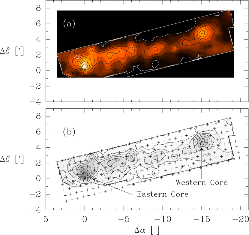
Figure 1: (a) Gaussian convolved map of visual extinction toward the northern streamer of IC 5146. Contours start at 4 mag of $A_{V}$ and increase in steps of 4 mag. The stars show the positions of IRAS point sources. (b) Points delineating the radio grid overlayed on the region surveyed in the infrared (as shown by the map of visual extinction). The near infrared survey region is outlined in each. The central reference position is listed in Table 1.

To enable a direct comparison between the near-infrared observations and the radio molecular-line observations (obtained with the FCRAO telescope and described in the next section), the mean near-infrared extinction along each line-of-sight associated with a molecular-line observation is calculated by convolving the individual infrared excess measurements with a two-dimensional Gaussian filter. The gaussian filter has a FWHM of 50″ to match the approximate beamsize of the FCRAO telescope, and is truncated at $r=3\sigma$. The uncertainty on the mean extinction is estimated from the Gaussian weighted rms dispersion of extinction measurements falling within each “beam.” The gaussian convolved map of visual extinction is shown in Figure 1a. This map is quite similar to the larger extinction map of IC 5146 presented by Lada, Alves, & Lada (1999).

2.2 Molecular-Line Observations

Over two separate observing periods (1999 March 23–25 and 2000 Jan 31 – Feb 01), the 14 m telescope of the Five College Radio Astronomy Observatory (FCRAO) in New Salem, MA was used to observe a $25\arcmin\times 8\arcmin$ region covering the Northern Streamer of the IC 5146 dark cloud. The rotational transitions of the following molecules were observed: ¹²C¹⁸O (109.782182 GHz, $J=1\rightarrow$ 0; hereafter, C¹⁸O), the hyperfine triplet of ¹²C¹⁷O (112.359277 GHz, $J=1\rightarrow 0$; hereafter, C¹⁷O – note that the two reddest components are blended and unresolved at our spectral resolution of 78 kHz; see below), ¹²C³²S (97.981011 GHz, $J=2\rightarrow$1; hereafter, CS), ¹²C³⁴S (96.412962 GHz, $J=2\rightarrow$1; hereafter, C³⁴S), ¹³C³²S (92.4979 GHz $J=2\rightarrow$1; hereafter, ¹³CS), and N₂H⁺ (93.173777 GHz, $J=1\rightarrow 0$). The N₂H⁺ transition consists of seven hyperfine components spanning 4.7 MHz; however, at our spectral resolution (78 kHz, see below) only the three main groups of lines centered at rest frequencies of 93.1719 GHz (a blend of three lines), 93.1738 GHz (a blend of three lines), and 93.1763 (a single line) are resolved (e.g., Caselli, Myers, & Thaddeus, 1995).

The observations reported in this paper were obtained with the newly commissioned SEQUOIA 16-element focal plane array receiver. The sixteen elements of the SEQUOIA array are aligned in a square $4\times 4$ pattern; each element is separated from its neighbor by 88″ in both the X and Y directions. A full beam sampled map requires 4 pointings of the array on the sky and is referred to as a “footprint”. All maps were centered with respect to $\alpha(J2000)=$ 21^h47^m27^s and $\delta(J2000)=$ 47${}^{\circ}31^{\prime}00^{\prime\prime}$.

The FAAS autocorrelator spectrometer was utilized in the 512-channel, 40 MHz bandwidth mode, yielding a channel spacing of 78 kHz ($\Delta v\sim 0.21$ km s^-1 at 112 GHz and $\Delta v\sim 0.25$ km s^-1 at 93 GHz) The 1999 data were taken in position switching mode, while the 2000 data were taken in frequency switching mode. For the frequency switched data, the signal frequency was shifted by 4 MHz. Typical system temperatures ranged from $140-300$ K. The integrations times for each molecule varied (see Table 1), but typical $T_{A}^{*}$ rms noise temperatures per channel were $\lesssim 0.02$ K. Internal calibration was done via a chopper wheel which allows switching between the sky and an ambient temperature load. Focusing and pointing were checked by observing periodically the SiO masers T Ceph (1999) and R Cas (2000). Typical, rms pointing uncertainties were 5″.

The Northern Streamer was mapped at full beam sampling in C¹⁸O, CS, and N₂H⁺. The $25\arcmin\times 8\arcmin$ map was rotated by 14^∘ North of East with respect to equatorial coordinates to follow the long axis of the cloud and the near-infrared survey data (e.g., Lada et al., 1994; Lada, Alves, & Lada, 1999). The full map required four “footprints” for a total of 256 grid points. The streamer contains two dense cores which are readily detectable in a 50^′′ beam and were mapped at full beam sampling in C³⁴S. The positions of the grid points in these two individual “footprints” are no different than the positions found in the the full map. A single additional “footprint” (64 grid points) was observed towards the eastern core in C¹⁸O. This “footprint” was offset from the regular map grid by $-0\farcm 369$ ($\sim 0.5$ beamsize) in both right ascension and declination. The purpose of this “footprint” was to increase the sampling of the C¹⁸O in the eastern core. Additional single array placements (16 grid points) on the eastern core were observed in C¹⁸O, C¹⁷O, and ¹³CS. These single array observations were used to investigate the C¹⁸O and CS optical depth of the core (see §3.1 and §3.2 below).

A summary of the map grid points is shown in Figure 1, and details of the observing parameters for each molecular observation can be found in Table 1. Several points on the southeastern edge of the radio grid fall outside of the infrared survey region and these data points are not included in this study.

For the remainder of the paper, the “Eastern Core” refers to the eastern-most “footprint” (i.e., the eastern-most $8\times 8$ grid), the “Western Core” refers to the western-most “footprint” (i.e., the western-most $8\times 8$ grid), and the “Mid-Streamer” refers to the two “footprints” ($16\times 8$ grid) lying between the “Eastern” and “Western” Cores (see Fig. 1).

All data were reduced using SPA and CLASS spectral line reduction packages in conjunction with custom-made analysis routines. A second order polynomial baseline was subtracted from the position-switch spectra; the frequency-switched spectra were folded and a second-order polynomial baseline was subtracted. Main beam efficiencies of $\eta_{MB}\approx 0.50-0.55$ were adopted from the SEQUOIA documentation. Final $T_{R}$ rms noise temperatures were generally $\lesssim 0.04$ K. All data presented in the paper are corrected using the main beam efficiency and are on the $T_{R}$ scale.

3 Results: Comparison of the Dust and Gas

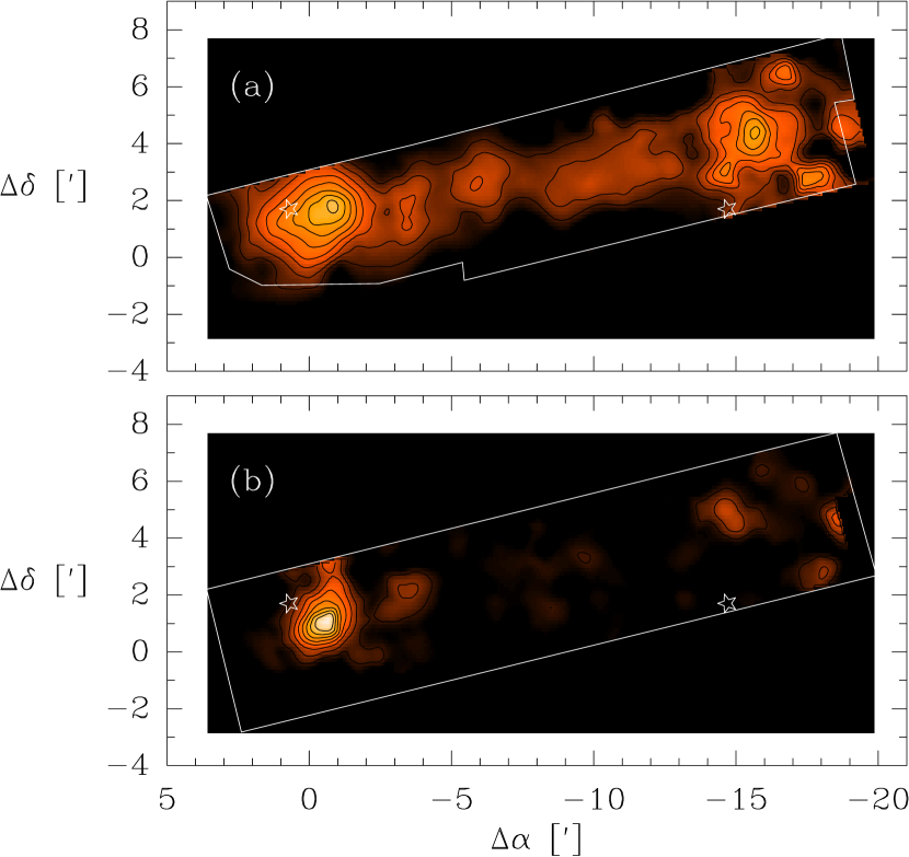
Figure 2: (a) Map of C¹⁸O J = 1 $\rightarrow$ 0 integrated intensity in IC 5146. Contour levels begin with 0.3 K-km/s and are spaced by 0.2 K-km/s. (b) Map of integrated N₂H⁺ J = 2 $\rightarrow$ 1 emission. Contour levels begin at 0.6 K-km/s and increase in steps of 0.6 K-km/s. The stars show the positions of IRAS point sources.

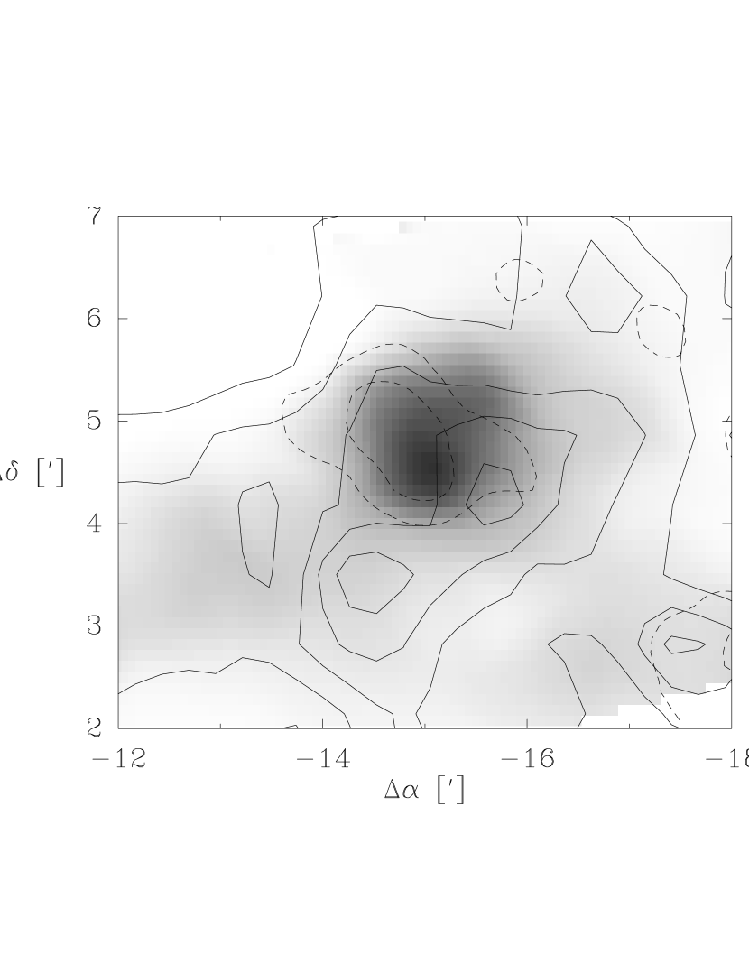
Figure 3: Comparison of C¹⁸O J = 1 $\rightarrow$ 0 integrated emission distribution (solid contours), N₂H⁺ J = 1 $\rightarrow$ 0 (dashed contours), with visual extinction (grey scale) towards the western core of the IC 5146 northern streamer. Note how the N₂H⁺ emission maximum corresponds with the peak of visual extinction. For C¹⁸O the contour levels begin with and are spaced by 0.3 K-km/s, while for N₂H⁺ contour levels begin with and are spaced by 0.6 K-km/s.

Figures 2a and b present maps of the integrated emission of C¹⁸O and N₂H⁺ in IC 5146. The map of C¹⁸O J $=1\rightarrow 0$ integrated intensity appears broadly similar in distribution to the visual extinction map shown in Figure 1. Both extinction and C¹⁸O trace column density enhancements, or cores, at the eastern and western edges of the mapped region, although the C¹⁸O emission peaks are slightly offset from those of $A_{V}$. The integrated emission of N₂H⁺ shows strong emission toward the eastern core, and only weak and somewhat clumpy distribution throughout the rest of the streamer. Curiously, the N₂H⁺ intensity appears to correlate reasonably well with the regions of highest extinction. This is more clearly demonstrated in Figure 3 where the integrated intensity distribution of N₂H⁺ and C¹⁸O are compared with visual extinction in the western core. Here the strongest N₂H⁺ emission appears directly on the peak of extinction, while the C¹⁸O emission maxima are offset by nearly 1^′. This is unlikely to be the result of differences in excitation requirements between these two transitions. The upper state energy of each transition is $\sim 5$ K and, while N₂H⁺ has a large critical density ($\sim 10^{5}$ cm^-3) and preferentially samples only the highest densities, the C¹⁸O emission should also trace the same density regimes. Instead these morphological differences are likely due to differences in the chemistry as will be discussed later in this paper.

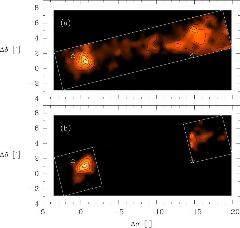
Figure 4: (a) Map of CS J = 1 $\rightarrow$ 0 integrated intensity in IC 5146. Contour levels begin with 0.5 K-km/s and are spaced by 0.5 K-km/s. (b) Smaller maps of the integrated C³⁴S J = 2 $\rightarrow$ 1 emission. Contour levels begin at 0.2 K-km/s and increase in steps of 0.1 K-km/s. The stars show the positions of IRAS point sources.

Figure 4 presents the total integrated emission for the J $=2\rightarrow 1$ transitions of CS and C³⁴S. The CS emission morphology is similar to that of C¹⁸O as CS strongly peaks on both cores and shows weak, but detectable, emission from the gas between the cores. Because of its weaker intensity, the J $=2\rightarrow 1$ transition of C³⁴S was only observed in the two cores. Within these smaller regions the C³⁴S emission is roughly similar to that of its more abundant isotope, CS.

In Figure 5 selected spectra at two different positions are presented. The two chosen positions are ($\Delta\alpha=+0\farcm 2$, $\Delta\delta=+0\farcm 7$) and ($\Delta\alpha=-0\farcm 9$, $\Delta\delta=+2\farcm 5$) are both associated with the Eastern core and sample extinctions that differ by a factor of two. Here we see that the intensity of C¹⁷O is significantly lower at the highest extinction (for $A_{V}$ = 36 mag the detection is 16$\sigma$ on the integrated intensity, while at $A_{V}$ = 19 mag the detection is 4$\sigma$). In contrast the emission of C³⁴S and N₂H⁺ appears to be stronger at the position with higher extinction. These differences, shown at only two positions, will be examined in greater detail with higher sampling in the following sections.

3.1 C¹⁸O

The direct comparison between the C¹⁸O integrated intensity and visual extinction at each point in the mapping grid is presented in Figure 6. The behavior of these two tracers is very similar to what was found previously for the IC 5146 region (Lada et al., 1994; Kramer et al., 1999). The integrated intensity and the extinction appear well-correlated for $A_{V}\lesssim 10-15$ mag. For $A_{V}\gtrsim 10-15$ mag, the relationship shows a high degree of scatter, and appears to flatten out.

A bivariate linear fit was performed for the data located at $A_{V}<10$ mag, with the following result:

$$I(C^{18}O)=\left(-0.4\pm 0.1\ K\ km\ s^{-1}\right)+\left(0.20\pm 0.01\ \frac{K\ km\ s^{-1}}{mag}\right)\cdot[A_{V}].$$ (1)

The above fit is in excellent agreement with the fit presented by Lada, Alves, & Lada (1999), for a similar region but at lower angular resolution (102″) than the observations presented here. The fit is also in agreement with the C¹⁸O-$A_{V}$ relationship found for the smaller region (and finer beamsize – 30″) studied by (Kramer et al., 1999). However, if the entire extinction range is used in the fit, the resulting slope is 15% shallower, consistent with earlier findings for both IC5146 (Lada et al., 1994) and also in L 977 (Alves, Lada, & Lada, 1999).

The two most likely effects which could explain the change in slope at high extinction are: (1) high C¹⁸O optical depth for $A_{V}\gtrsim 10$ mag, and (2) depletion of CO onto the surface of dust grains. A third possibility is a decrease of the CO excitation temperature to $T_{ex}<5$ K for $A_{V}\gtrsim 10$ mag. However, Alves, Lada, & Lada (1999), for a similar result in L 977, make a convincing argument that this is not a likely possibility. They argue that heating mechanisms (cosmic ray rates, ambipolar diffusion, and natural radioactivity) are sufficient to prevent the gas in cloud cores to cool below 5 K. Although we cannot completely rule out this possibility, we regard the cooling of the gas to such extreme temperature as unlikely, and proceed with a discussion of the optical depth and depletion.

The paired C¹⁸O–C¹⁷O single pointing observations provide information regarding the optical depth of the C¹⁸O in the densest portions of the eastern core (see Table 1). C¹⁸O and C¹⁷O should be collisionally excited under the same physical conditions deep inside cold cores where the molecules are well-shielded from external ultraviolet radiation (Ladd, Fuller, & Deane, 1998; van Dishoeck & Black, 1988). Additionally, the ratio [¹⁸O]/[¹⁷O]$=3.65\pm 0.15$ appears to be relatively constant throughout the interstellar medium (Penzias, 1981). Thus, the only difference in the emission between C¹⁸O and C¹⁷O should arise from the oxygen relative abundance; i.e., completely optically thin emission of C¹⁸O and C¹⁷O should have an integrated intensity ratio of 3.65.

A comparison of the integrated intensities of C¹⁷O vs C¹⁸O is shown in Figure 7 (top). The solid line represents the expected ratio of 3.65 for optically thin emission and does not represent a best fit to the data. The dashed lines represent the $1\sigma=\pm 0.15$ uncertainty of the [¹⁸O]/[¹⁷O] ratio. The excellent agreement of the data distribution with the predicted ratio indicates that the C¹⁸O emission is indeed optically thin.

To test directly for optical depth effects as a function of total column density, the C¹⁸O/C¹⁷O ratio has been plotted as a function of extinction (bottom, Fig. 7). The extinction provides an independent assessment of the total column density along each line of sight. If the C¹⁸O was optically thick at high column density (high extinction), the C¹⁸O/C¹⁷O ratio should systematically decrease as a function of increasing extinction. The ratio is remarkably constant over a range of 40 magnitudes of visual extinction. Figure 7 implies that (1) the [¹⁸O]/[¹⁷O] ratio in IC 5146 is very near the previously determined interstellar value of $3.65\pm 0.15$, and (2) the C¹⁸O emission is not highly optically thick. However, due to the errors on the ratios we cannot rule out the C¹⁸O emission being thin, but with moderate optical depth ($\tau\lesssim$ 0.5 ).

The ratio of the three hyperfine components of C¹⁷O can be used to determine whether or not C¹⁷O is thin. The relative intensities of the three components (central:blue:red) are 4:3:2 for optically thin emission (Ladd, Fuller, & Deane, 1998). At the spectral resolution of our data (78 kHz), the central and red components are blended; thus, the measured relative intensity of the two components (central-red blend:blue) should be 2:1, for optically thin emission and indeed the measured median relative intensity is $2\pm 0.5$. If this is the case then the difference in the two C¹⁷O spectra presented in Figure 5, with the highest extinction having lower emission, is suggestive of a drop in abundance.

3.2 CS

The depletion of sulfur bearing molecules (e.g., CS and SO) is predicted to be a sharp function of the density, and these species should be robust tracers of gas phase molecular depletion on to the surface of dust grains in cloud cores (Bergin & Langer, 1997). As there was already evidence to suggest that CO may be depleted in the cores of IC 5146 (§3.1), CS should also show evidence for gas-phase depletion.

To explore this hypothesis, the C³⁴S optical depth was computed for both the eastern and western cores at positions where we have observations of both CS and C³⁴S, using the following relationship:

$$\frac{\rm T(C^{34}S)}{\rm T(CS)}=\frac{1-\exp{[-\tau]}}{1-\exp{[-a\tau]}},$$ (2)

where $\tau$ is the C³⁴S optical depth and $a$ is the abundance ratio of $[^{32}\rm{S}]/[^{34}\rm{S}]=14$ (Pratap et al., 1997). Using the ratio of the integrated intensities, we iteratively solved Equation 2 for $\tau$, until the calculated intensity ratio matched the measured intensity ratio to within $\sim$5%. In Figure 8, the C³⁴S optical depth is shown as a function of visual extinction $A_{V}$. The uncertainties shown in Fig. 8 are a result of the uncertainties in the integrated intensity measurements; the uncertainties associated with the convergence of the numerical calculations are significantly smaller. The derived opacities clearly indicate that the emission from C³⁴S is optically thin in both cores for all A_V. However, the emission from CS ($\tau_{\rm CS}=\tau_{\rm C^{34}S}*14$) must be optically thick throughout the cloud. Surprisingly, despite being thin, the C³⁴S optical depth is nearly constant for $A_{V}\gtrsim 10$ mag.

As a check of the derived optical depths, the optical depth of ¹³CS was calculated in a similar manner to the C³⁴S optical depth. Only the position ($-0\farcm 54,0\farcm 89$) was sufficiently strong to permit such a calculation ($\int T(^{13}{\rm CS})dv=0.089\pm 0.02$ K km s^-1). An optical depth of $\tau=0.033\pm 0.008$ was found, implying that the C³⁴S optical depth (assuming an abundance ratio of $[\rm{C}^{34}S]/[^{13}\rm{CS}]=4.29$) is $\tau=0.14\pm 0.03$ (see Fig. 5). The C³⁴S optical depth measured using the T(C³⁴S)/T(CS) ratio is $\tau=0.14\pm 0.04$, at the same position, confirming the small opacities of C³⁴S in this cloud.

Examining the dependence of C³⁴S opacity with extinction in Figure 8 we find that while the extinction rises by a factor of 2.5 ($15-40$ mag), the C³⁴S optical depth remains nearly constant at $\tau\approx 0.15-0.25$. Indeed, there is even a small hint that the optical depth of the C³⁴S in the eastern core is decreasing as a function of increasing extinction. The eastern core also appears to have an opacity that is, on average, slightly higher than the western core. As optical depth is a direct tracer of column density in either the upper or lower state, this difference suggests that the abundance of CS could be different between the two cores. Moreover, the constant opacity with extinction for both cores would then be indicative of a C³⁴S(and CS) abundance decrease with increasing extinction. However, CS and C³⁴S have high dipole moments and their emission is sensitive to gas density, as opposed to C¹⁸O emission which is fairly insensitive to the density (provided n${}_{H_{2}}$ $>1000$ cm^-3). Thus, for CS and its isotopic variants, changes in the excitation conditions can play an important, and with regards to depletion analyses, potentially confusing role. These effects are examined in §4.

3.3 N₂H+

Unlike CS, or even CO, N₂H⁺ is predicted by evolutionary chemical models to have a low depletion rate, due to the relatively low binding energy of its precursor molecule, N₂ (Bergin & Langer, 1997). Thus, we might expect that N₂H⁺ would exhibit a different behavior as a function of extinction when compared to CS or CO.

In Figure 9, the the N₂H+ integrated intensity, summed over all hyperfine transitions, is compared to the visual extinction. This figure clearly shows quite a different relationship between N₂H⁺ integrated emission and visual extinction when compared to the other species included in our study. For $A_{V}\lesssim 15$ mag, the N₂H+ integrated intensity vs $A_{V}$ is nearly flat and follows the following relationship:

$$I(N_{2}H+)=\left(-0.03\pm 0.04\ K\ km\ s^{-1}\right)+\left(0.017\pm 0.006\ \frac{K\ km\ s^{-1}}{mag}\right)\cdot[A_{V}]\ (A_{V}<15\ {\rm mag}).$$ (3)

Note that the slope of the linear fit is non-zero at the 3$\sigma$ level, indicating that the N₂H+ intensity gradually increases with extinction. At $A_{V}\gtrsim 15$ mag, the intensity displays a sharp increase and the N₂H+$-A_{V}$ relationship steepens by nearly a factor of 15:

$$I(N_{2}H+)=\left(-4.3\pm 0.6\ K\ km\ s^{-1}\right)+\left(0.26\pm 0.03\ \frac{K\ km\ s^{-1}}{mag}\right)\cdot[A_{V}]\ (A_{V}>15\ {\rm mag}).$$ (4)

Curiously, the increase in N₂H⁺ intensity occurs at a similar visual extinction to where the CO-$A_{V}$ relationship begins to show evidence of potential depletion. The derivation of N₂H⁺ abundances and the physical cause for the sharp increase at $A_{V}$ $\gtrsim 15$ will be discussed in the following section.

4 Analysis: Molecular Excitation and Abundances

In the previous section we searched for correlations between integrated emission and visual extinction for each of the surveyed molecules. Here we examine whether any departures from the correlation are the result of excitation and/or abundance gradients. In this section we concentrate on trends in relative or normalized abundances (i.e. abundances normalized using the abundance derived at the lowest extinction with reliable data points). In this fashion, in the determination of molecular abundance for a given species, we eliminate common uncertainties (such as collision rates).

To calculate total column densities from the molecular data we account for the radiation transfer through the use of the large-velocity gradient approximation. To reduce the effects of opacity we use here only the C¹⁷O, C³⁴S, and N₂H⁺ data. Since the emission of C¹⁷O and C³⁴S (§3.1 and 3.2) is optically thin, and, based upon ratios of hyperfine components, much of the N₂H⁺ emission is also thin, this reduces the LVG approximation to simply solving the equations of statistical equilibrium. The results are therefore less dependent on the details of the radiative transfer solution. To improve the statistics of our results we average abundances in bins of 5 magnitudes starting with $A_{V}$ = 5 mag. Below this value there are little or no significant ($>3\sigma$) data points (for N₂H⁺, C¹⁷O, and C³⁴S).

In this study we observe only a single transition of a given molecular species. However, in each case we have information on the optical depth, using CS for C³⁴S, and the hyperfine ratios for C¹⁷O and N₂H⁺. This provides an additional and limiting constraint on the column density determination. With the observed intensity and opacity from a single transition the total column density can be derived with knowledge of the collision rates, density, temperature, and line width. The collision rates are available from the literature and the line width or velocity dispersion is an observed quantity. However, to derive a map of the total column density from the molecular line maps requires a priori knowledge of the density and temperature structure of the IC 5146 cloud.

For the density structure we use the analysis in (Lada, Alves, & Lada 1999; hereafter LAL99) who show that the extinction (or column density) gradient in the same region of IC 5146 is nicely reproduced by a cylindrical geometry (for the entire streamer) with $\rho\propto r^{-2}$. The procedure LAL99 use to determine the density structure is identical to the commonly used method of deriving the volume density structure from mm and sub-mm dust continuum emission (see Shirley et al 2000 and references therein). To be consistent with the results in LAL99, which show a large systematic increase in volume density from low to high extinction, we adopt the following density profile (n${}_{H_{2}}$ $=$ n${}_{H_{2}}$(r = r₀) $\times$ (r₀/r)² $=10^{5}$(0.047 pc/r)² cm^-3). The density profile is shown in Figure 10 and is in reasonable agreement with the radial profile of total column density (Figure 8 in LAL99). In our calculations we use average densities in bins of 5 mag (shown as horizontal hash marks in Figure 10). For example, if a given data point has an extinction between 5 and 10 mag then we use the average density of n${}_{H_{2}}$ $=1.4\times 10^{4}$ cm^-3 within that bin.

There exists some information on the temperature structure from observations of CO and NH₃. CO observations generally show gas temperatures ranging from 10 to 13 K (Dobashi et al., 1992). However, these estimates are likely reflective of the temperature at the cloud surface and not the denser interior (Bergin et al, 1994). In the eastern core NH₃ observations provide some information on the dense gas temperature with T = 13 K (Jijina, Myers & Adams, 1999). We also have a single detection of the J = 6 $\rightarrow$ 5 (K = 0 and 1) transition of CH₃C₂H, which can be used to estimate the temperature (Bergin et al, 1994). Since this detection is at a single position ($\Delta\alpha=-0\farcm 5$, $\Delta\delta=+0\farcm 9$) we have not shown the spectra; however, the K = 0 integrated intensity is $\int T\delta v=$ 0.11$\pm 0.02$ K km s^-1 and K = 1 is $\int T\delta v=$ 0.13$\pm 0.02$ K km s^-1. Using the method described in Pratap et al. (1997) the ratio of these two is consistent, within the errors, with a gas temperature $<13$ K. Given this information, it is unlikely that there are strong temperature gradients throughout most of the IC5146 molecular streamer with the probable range between (perhaps) 5 and the CO temperature of 13 K. In the following we present abundances calculated with a constant temperature of 10 K and discuss the results of additional analysis assuming constant temperatures of 5 and 13 K (and combinations thereof).

4.1 C¹⁷O Abundance

Because of concerns that moderate opacities in C¹⁸O emission could potentially mask small abundance changes in order to search for relative abundance differences we predominantly use the more limited C¹⁷O observations. For the C¹⁷O column density derivation, we use the collision rates of CO with para-H₂ (Flower, 1988). We adopt the density determined as a function of extinction as described above and the temperature is assumed to be constant at 10 K for each position (changes in the temperature will be discussed below). The line width is determined via gaussian fits to each spectrum. Because the C¹⁷O J $=1\rightarrow 0$ transition has hyperfine structure we use this additional information in our derivation of column density. We therefore simultaneously fitted the two resolved hyperfine components (as discussed in §3.1 the F $=7/2\rightarrow 5/2$ and F = $=3/2\rightarrow 5/2$ are blended), assuming that the hyperfine levels are populated according to LTE. The two constraints on the on the $\chi^{2}$ search for the best fit column density are: (1) the intensity of the lines and (2) the relative intensities of the hyperfine ratios which limits the opacity of the solution. In general the reduced $\chi^{2}$ of most solutions are $<1$ and in all cases the C¹⁷O emission is found to be optically thin. For each position we derive column densities if the observed integrated intensity is $>3\sigma$. The abundance relative to H₂ is derived using N${}_{H_{2}}=10^{21}$$A_{V}$.

Table 3 presents the weighted average abundance of C¹⁷O (within 5 mag bins of extinction) and in Figure 11 the relative abundance of C¹⁷O is given as a function of visual extinction. In this figure we normalize the abundance to the lowest extinction bin with a statistically significant abundance determination (between 5 and 10 mag). Excluding the point at $A_{V}$ = 27.5 mag with large errors, we see that the relative C¹⁷O abundance shows a steady and significant decrease, by a factor of 3, from the lowest to highest visual extinction. This result is found assuming a constant temperature of 10 K. To investigate whether a systematic temperature gradient can change the result we repreated the same procedure assuming constant temperatures of 5 and 13 K. To mimic temperature gradients we examined combinations of these results. In the absence of a significant population of luminous embedded stars (the case here) the most likely systematic temperature gradient is the temperature decreasing with increasing extinction. In this case we find that the C¹⁷O abundance at high $A_{V}$ (with T = 5 K) does increase due to higher opacity in the J = 1 state, allowing for greater column density, but by only 15%. At the cloud edges (provided T = 13 K) the abundance also shows a slight increase, primarily due to the lower population in the J = 1 state. If the temperature were even greater then the abundance continues to rise. In all, this examination still provides a factor of 3 decrease in the C¹⁷O abundance from $A_{V}$ = 5 to 40 mag. It is worth emphasizing that even if CO and its isotopic variants are completely depleted in the dense core center the molecular observations will detect emission from the relatively undepleted gas residing in the low density regions along the line of sight through the core. Thus, if CO shows evidence for depletions at 10 mag in a cloud with a total extinction (from Fig 5 for example) of 40 mag, then the measured abundance will drop by at most a factor of four.

A similar analysis was performed using the entire C¹⁸O data set and we find that the relative abundance is essentially constant until the highest extinction bin, whereupon the abundance decreases by a factor of 1.5. This confirms our suspicion that the C¹⁸O emission is likely to have moderate optical depth ($\tau\sim 0.5$) which masks the larger abundance difference (factor of 3) seen in C¹⁷O. We note that one core in our data set ($\Delta\alpha=-9\farcm 2$, $\Delta\delta=2\farcm 9$) has been examined with the IRAM 30m antenna at higher ($\sim 30^{\prime\prime}$) resolution by Kramer et al. (1999). They find a clear decrease in the CO abundance near 12 mag. Our results are not as dramatic as found in the higher resolution study, which allowed for more data points to be placed at higher extinctions. For instance, the Kramer et al. (1999) core shows a peak extinction in a 30^′′ beam of $\sim 28$ mag, at a resolution of 50^′′ this reduces to a peak extinction of 16 mag. Thus, our sampling is lower in the exact regions where gas-phase depletions are most likely.

4.2 C³⁴S (and CS) Abundance

To derive the total column density of C³⁴S we use a similar method described for C¹⁷O in the previous section. That is, with a density and temperature assumed (and constant) for each grid position we perform a $\chi^{2}$ search for the best fit total column density. For collision rates we use the rates given by Green & Chapman (1978), and the line width is determined via gaussian fits to the spectrum. C³⁴S does not have hyperfine structure, but we have additional information in that the C³⁴S opacity has been determined for all positions with $>3\sigma$ integrated intensities (§3.2). Thus, for each data point we again two constraints for the radiative transfer model: (1) the integrated intensity and (2) the opacity of the J $=2\rightarrow 1$ transition. The majority of column density solutions have reduced $\chi^{2}<1$.

The C³⁴S integrated intensity as a function of visual extinction is presented in Figure 12. This Figure is notable in that the C³⁴S integrated intensity appears to be reasonably well correlated with $A_{V}$. This result is somewhat surprising given the near constant opacity as a function of extinction shown in Figure 8. The near uniform opacity would suggest that the C³⁴S (and therefore CS) abundance is sharply decreasing with extinction. However the dependence in Figure 12 is at odds with that conclusion, as it requires a constant abundance. This difference, an integrated intensity correlated with $A_{V}$, combined with a constant optical depth, can be reproduced, provided that there was a change in excitation from low to high extinctions. Indeed we can expect such a increase in the C³⁴S excitation temperature proceeding from lower to higher $A_{V}$, as a direct result of the known density gradient. Even a small change in the excitation temperature could replicate the observed dependence.

The results of the C³⁴S excitation analysis are presented in Table 3 in the form of abundances and in Figure 11 as normalized abundance plotted against visual extinction. Examining the data points we find a steady statistically significant abundance ($>3\sigma$) decrease by an overall factor of 3 from low to high extinction. Thus, by accounting for the rise in density as required by the NIR observations, and the observed constant opacity, along with an integrated intensity that increases with extinction, we find that the CS abundance decreases with $A_{V}$. If we assume that the most likely temperature gradient is with warm gas at core edges (T = 13 K) and cold gas (T = 5 K) in the center then the abundance still systematically declines by a factor of 2. In all, these results suggest that CS, like CO, shows an abundance decrease in the dense gas likely due to depletion onto grains.

4.3 N₂H⁺ Abundance

To derive the abundance of N₂H⁺ we use the total intensity of the lines along with the hyperfine ratios as described earlier for C¹⁷O. We use the collisional rates for HCO⁺ excited by para-H₂ (Flower, 1999), which has comparable collisional rates to N₂H⁺ (Monteiro, 1984). The results of the excitation calculations are given in Table 3 and shown in Figure 11.

First, there are only 3 N₂H⁺ detections between 0 and 5 mag of extinction, and of these, two have $A_{V}$ $>$ 4.5 mag (these data are not provided due to high errors). Although C³⁴S and C¹⁷O also have little emission in this regime, the more abundant isotopes, C¹⁸O and CS, both are detected at low extinction. Thus, unlike for other species, there appears to be little N₂H⁺ below $A_{V}$ $\lesssim$ 4 mag. Beyond the lowest extinctions, for T = 10 K the N₂H⁺  normalized abundance in Figure 11 shows a high abundance for low $A_{V}$ ($\sim 7.5$ mag) then decreases by a factor of 3 for $A_{V}$ = 17.5 mag, whereupon the abundance increases by a similar factor at high $A_{V}$. In our solutions with different temperatures (T = 5, 10, and 13 K) we find that the initial abundance decrease for $A_{V}$ $<17.5$ mag is lessened, provided that the cloud is warmer in these regions. If the gas is cooler in the core center then we find an even greater increase in relative abundance for $A_{V}$ $>17.5$ mag.

In summary we find, at least, two regimes for the N₂H⁺ abundance: (1) there is a threshold of extinction, $A_{V}^{th}\lesssim 4$ mag below which we find little or no N₂H⁺ in the gas-phase and (2) for higher extinctions the abundance shows a complicated structure that initially declines in value until $A_{V}$ = 15 mag whereupon it the relative abundance increases with extinction. Consideration of potential temperature changes reduces the initial decline, but would increase the rise in relative abundance towards to the core center. However, there is no evidence for a systematic decrease in the N₂H⁺ abundance at large $A_{V}$. In the following section we examine the physical and chemical causes that give rise to this dependence.

5 Discussion

5.1 Differential Molecular Depletions in IC 5146

In the preceding section we examined the excitation of the three molecules included in our survey. The results of this analysis is that we find good evidence for the presence of differential molecular depletions in IC 5146. That is, C¹⁸O and CS (and C³⁴S) are depleting from the gas phase at high extinctions and N₂H⁺ is not (at least at a resolution of 50^′′). Similar evidence of differential depletions are found in the literature, for a summary see Bergin (2000). The depletion of CCS relative to both ammonia and N₂H⁺ (with the latter two tracers typically coincident with the dust continuum emission peak) found in isolated low-mass cores is quite similar to the results found in our work (Kuiper, Langer, & Velusamy, 1996; Ohashi et al., 1999). Recently, Caselli et al. (1999) found evidence of CO depletion in the starless L1544 cloud core in a region traced by both N₂H⁺ and dust continuum. The detection of gas phase molecular depletions should not be considered as unexpected, given that molecular ice features have been observed along numerous lines of sight in the ISM (Whittet, 1993; Tielens et al., 1991).

In general, previous searches for chemical differences related to molecular depletion relied on finding morphological dissimilarities between the emission of two or more species with each other or with dust continuum (similar to that shown in Figure 3) and then performing an excitation analysis to prove or disprove that such differences are the result of chemical abundance variations. Our study has found comparable results, but has placed the evidence for molecular abundance changes, which are attributed to depletion, on firmer statistical grounds and removes any ambiguity in terms of the total hydrogen column density, such as those associated with using dust continuum emission (Kramer et al., 1998).

5.2 Comparison with Chemical Theory

This depletion pattern with sulfur bearing molecules (e.g. CS, CCS), along with CO, showing depletions onto grains and N₂H⁺  remaining in the gas-phase is in good agreement with the theoretical models presented by Bergin & Langer (1997). In these models, the gas-phase chemistry includes the effects of molecules both depleting onto and evaporatoring from grain surfaces. N₂H⁺ remains in the gas-phase longer at higher densities than other molecules because the high volatility of its pre-cursor molecule, N₂, allows for various desorption mechanisms (such as thermal evaporation or cosmic-ray spot heating of grain surfaces) to keep a significant N₂ abundance, and therefore N₂H⁺, in the gas phase at high densities.

To compare our results with the gas-grain chemical model of Bergin & Langer (1997), we use the density profile given in Figure 10. This profile matches the one derived for IC 5146 from the NIR extinction measurements (LAL99). We adopt the notation $\tau_{V}$ with regards to cloud depth because the model is computed using cloud radius, thus $A_{V}$ $=2\tau_{V}$. With extinction and density (we also assume a constant dust and gas temperature of 10 K and a UV enhancement factor of $G_{0}=2.2$; Kramer et al 1999) predetermined as a function of radius, we use the chemical model of Bergin & Langer (1997) to predict abundances as a function of both time and visual extinction and then directly compare these to the observational results. This model is slightly different from Bergin & Langer (1997) in that we do not allow for the density to evolve with time, but rather hold the density constant for each radius (and therefore extinction). However, the density does increase with increasing extinction, properly matching the observed structure.

Figure 13 presents two different chemical models. The top two panels show a pure gas-phase chemical model sampled at two different times ($10^{5}$ and 10⁷ yr). This model includes the effects of grain absorbing UV radiation (thereby allowing for molecular formation) but does not include any gas-grain interactions. We note that to match the models to observations $\tau_{V}$ must be multiplied by a factor of two to account for both sides of the cloud (i.e. the model was done using radius and not diameter). In Figure 13, we see that the abundances of most species rise as the UV radiation field is attenuated with increasing extinction and then remain constant. This behavior exists despite the nearly two order of magnitude rise in density from edge to center. However, for N₂H⁺ there is a slow steady decrease in abundance towards greater extinction. This behavior is readily understood by examining the primary formation and destruction processes for N₂H⁺. Using the pathways outlined in Appendix A, we see that the formation rate of N₂H⁺ (via cosmic ray ionization) should be essentially constant with density, with the assumption that cores are threaded by cosmic rays. However, due to the higher probability for collisions with higher density, the destruction rate via dissociative recombination and reactions with CO is raised. Thus, for pure gas-phase models the prediction is that the abundance of N₂H⁺ decreases with extinction.

The second model shown in the bottom two panels of Figure 13 is a gas-grain chemical model where molecules are allowed to collide and stick to the surfaces of dust grains. The primary desorption mechanism is cosmic-ray spot heating. For the binding energy of molecules to the grain surfaces we assume that the grains are coated by a layer of CO molecules. For more details of the model see Bergin & Langer (1997). Comparing the pure gas-phase model with the gas-grain model at t = 10⁵ yr the abundance profiles are similar. At this early time depletion has yet to play a role. For later times, we see demonstrative effects due to grain depletion: (1) for $\tau_{V}>6$ mag ($A_{V}$ $>12$ mag) the abundance of CS is dramatically reduced (2) the abundance of CO shows a small, factor of $\sim$3, decrease between $\tau_{V}$ $=0$ to 16 mag and (3) the abundance of N₂H⁺ is constant with $A_{V}$. For N₂H⁺ this behavior is in direct contrast to that seen in the pure gas-phase case. This indicates that the N₂H⁺ destruction rate must be progressively lower with higher extinction and density in the gas-grain model than for pure gas-phase chemistry. From Appendix A the major destroyers of N₂H⁺ are CO and electrons. In Figure 13 there is increasing CO depletion with higher density and extinction which results in a progressively lower N₂H⁺ destruction rate. Thus, the observed uniform abundance of N₂H⁺ at high extinctions is also a direct consequence of CO depletion and is not solely the result of the high volatility of the N₂ molecule. It is worth noting that if more CO molecules freeze onto grains, as would occur when time progresses, then N₂H⁺ abundance rises accordingly.

Finally, we note that at low $A_{V}$, for CS and CO (x(C¹⁸O) $\times$ 500), the models can be directly compared to the observed abundances and predicted values are in reasonable agreement with observations (compare Figures 11 and 13). For high $A_{V}$, the models, as presented here as abundance profiles with extinction, cannot be directly compared to the observations. This is because the observations are averages over the entire line of sight, including both depletion zones and undepleted gas. For a direct comparison, the chemical model would have to be averaged over the line of sight, stepping through $A_{V}$, in similar fashion to the observations. However, this is not the case for undepleted species (e.g. N₂H⁺), which can be directly compared to observations. If the relative abundance profile in Figure 11 is correct then the observations would suggest a combination of undepleted models (to account for the low $A_{V}$ decline in abundance) and the depleted models (accounting for the rise in abundance at high extinction) would be required. In each case the models are in reasonable agreement with the overall value of abundance.

5.3 Testing Interstellar Photodissociation Rates

In §4.3 we found two regimes for the N₂H⁺ abundance: (1) there is a threshold extinction, $A_{V}^{th}\lesssim 4$ mag, below which there is little or no N₂H⁺, and (2) for higher extinctions the abundance is roughly constant. In the previous section we discussed how the structure in latter regime can be reproduced. However, in Figure 13 the dependence found in the former regime is also addressed. In the chemical model the lack of N₂H⁺ for $A_{V}$ $\lesssim 4$ mag is the result of the photodissociation of its parent molecule (N₂), combined with a higher electron abundance at cloud edges due to photoionization. In Figure 13, N₂H⁺ shows a sharp rise in abundance for $\tau_{V}\sim 3$ mag, corresponding to $A_{V}$ $\sim 6$ mag. This is quite close to the observed threshold. The N₂ photorate is taken from van Dishoeck (1988), where the depth dependence of the photodissociation rate depends on its absorption cross section, the assumed radiation field, the continuum attenuation, and on the albedo and scattering phase function of the grains (van Dishoeck, 1988). Despite the complications involved in this computation, given the match between the observed and predicted threshold, the depth dependence of the rate and the ionization structure, appears to be reasonably taken into account.

We note that the chemical model in Figure 13 does not properly account for the self-shielding of CO molecules, as C¹⁸O is emission is observed for $A_{V}$ $<4$ mag (Figure 6). However, the effect of increased CO shielding in the model would be to lower the electron abundance at the cloud edge and increase the importance of N₂ photodestruction as the method for lowering the N₂H⁺ abundance. Our assertion that N₂ photodissociation is contributing to the observed N₂H⁺ abundance threshold would then be strengthened.

van Dishoeck (1988) present a different photorate computed using a different grain model than used in our model, one with the grains more forward scattering (their grain model 3). If we use the depth dependent photorates from that model (for all steps in N₂ and N₂H⁺ production) we find that the N₂ photodissociation rate is larger deeper into the cloud and the N₂H⁺ threshold shifts to beyond $A_{V}$ = 10 mag. This is in disagreement with the observations and points to an important use of the technique outlined in this paper. In the future, by observing and modeling clouds with simple and well-characterized structure, the depth dependent photorates (along with the gas-grain interaction) can be tested. Indeed, most of the depth dependent photorates for many molecules are highly uncertain (van Dishoeck, 1988). In some cases this is due to a lack of viable cross-sections, but also because the detailed rate calculations could not be observationally verified. Although, there certainly are complications in application; this technique offers a viable opportunity to provide observational tests of these rates, which can help in constraining not only the depth dependence of the photorates but also the grain physics.

6 Summary

We have examined the correlation of the emission of three molecules: C¹⁸O, CS, and N₂H⁺ with visual extinction in the northern streamer of the IC 5146 cloud. We use the molecular data, along with a model of the excitation, to determine molecular abundances and examine the abundance profile with $A_{V}$. The principle results are:

(1) We find good evidence for a reduction in the abundance of CO and CS (using C³⁴S) for $A_{V}$ $\gtrsim 10-15$ mag. This reduction is attributed to the depletion of these molecules onto the surfaces of cold dust grains in the densest portions of the IC 5146 cloud.

(2) For N₂H⁺, we find two separate regimes for its abundances: (a) for low extinction there is a threshold extinction, $A_{V}^{th}\lesssim 4$ mag, below which little N₂H⁺ is found and (b) for $A_{V}$ $\gtrsim 4$ mag the N₂H⁺ abundance is either constant or declining until $A_{V}$ = 15 mag whereupon the abundance rises as a function of extinction in the visual.

(3) We find that density gradients in cloud cores can have a profound effect on the derivations of the spatial distributions of total column densities and molecular abundances for species with high dipole moments. Chemical interactions, such as reaction rates and depletion timescales, are also strongly density dependent. Thus the interpretation and determination of accurate abundances in dense cloud cores requires both knowledge of the density and temperature structure in the cloudy material and a proper accounting for such structure in abundance determinations and chemical models.

(4) The observed patterns of differential depletion shows CS and CO exhibiting molecular depletions while N₂H⁺ remains in the gas phase. This is in good agreement with the predictions of chemical theory by Bergin & Langer (1997).

(5) By combining the observationally derived density profile for IC 5146 from Lada, Alves, & Lada (1999) with the gas-grain chemical model of Bergin & Langer (1997), we show that the observed constant N₂H⁺ abundance with extinction can be reproduced provided that CO, which is a major destroyer of N₂H⁺, is depleting in the dense cores. Since CO depletion is observed this result is an important clue to the physical and chemical reason that allows N₂H⁺ molecules to trace the densest regions of molecular cores.

(6) We also demonstrate that the observed N₂H⁺ abundance threshold ($A_{V}^{th}\lesssim 4$ mag) is partially due to the photodissociation of N₂. This highlights an important application of this technique, which is the ability to test not only the chemical models of dense regions, and thereby directly probe the gas-grain interaction, but also to provide a viable and completely new method for observationally testing models of depth-dependent photodissociation rates.

Appendix A Formation of N₂H⁺ Abundance

The primary route to form N₂H⁺ is through the following reaction:

$$\rm{H_{3}^{+}+N_{2}\rightarrow N_{2}H^{+}+H_{2}}.$$ ()

H${}_{3}^{+}$ is the produced via cosmic ray ionization of H₂. The main destruction pathways are dissociative electron recombination and a reaction with CO (reactions with O and C are of lesser import). In equilibrium, the following expression can be derived for the concentration of N₂H⁺,

$$\rm{n(N_{2}H^{+})=\frac{n(H_{3}^{+})n(N_{2})k_{H_{3}^{+},N_{2}}}{n(e^{-})\alpha(N_{2}H^{+})+n(CO)k_{CO,N_{2}H^{+}}}}.$$ ()

Where $\alpha(\rm{N_{2}H^{+}})$ is the dissociative recombination coefficient and k${}_{\rm{x,N_{2}H^{+}}}$ are the various reaction rates given by Millar, Farquhar, & Willacy (1997). See also Womack, Ziurys, & Wyckoff (1992).

Figure 5: Plot showing selected spectra at two different positions in the Eastern core: ($\Delta\alpha=+0\farcm 2$, $\Delta\delta=+0\farcm 7$) with $A_{V}$ = 36 mag and ($\Delta\alpha=-0\farcm 9$, $\Delta\delta=+2\farcm 5$) with $A_{V}$ = 19 mag.

Figure 6: C¹⁸O integrated intensity vs. visual extinction for the entire Northern Streamer. The best fit linear relationship for $A_{V}\leq 10$ mag is given as the solid line, and is extrapolated as the dash-dot line for $A_{V}>10$ mag. The median uncertainties in the measurements are shown in the lower-right corner. The eastern core, western core, and mid-streamer are plotted as different symbols as indicated by the legend.

Figure 7: Comparison of the C¹⁷O and C¹⁸O integrated intensities in the eastern core. The solid line represents the expected trend ($\pm 1\sigma$ – dashed lines) for optically thin emission. (b) C¹⁸O–C¹⁷O ratio of integrated intensities vs. visual extinction. The solid line represents the expected ratio for optically thin emission. The dashed lines represent the median $1\sigma$ uncertainty of the measured ratios.

Figure 8: C³⁴S optical depth vs. visual extinction for the eastern and western cores. The eastern core and western core are plotted as different symbols as indicated by the legend. The circle ($\circ$) at $A_{V}\approx 27$ mag represents the optical depth as derived from the ¹³CS data. The C³⁴S optical depth measured for that same line of sight overlaps the ¹³CS derived optical depth.

Figure 9: N₂H+ integrated intensity vs. visual extinction for the entire Northern Streamer. The best fit linear relationship for $A_{V}<15$ mag is plotted as the dashed line, and the best fit linear relationship for $A_{V}>15$ mag is plotted as the solid line. The median uncertainties in the measurements are shown in the lower-right corner. The eastern core, western core, and mid-streamer are plotted as different symbols as indicated by the legend.

Figure 10: Volume density of molecular hydrogen as a function of visual extinction and radius. This profile is in good agreement with the profile of extinction with cloud radius determined in Lada, Alves, & Lada (1999). The horizontal hash marks found along the line representing the density profile are the average densities used in the molecular abundance analysis for respective bins of 5 mag starting with $A_{V}$ = 5 – 10 mag.

Figure 11: Normalized molecular abundances derived from combined molecular column densities and NIR extinction measurements of C¹⁷O (circles and solid line), C³⁴S (squares and dashed line), and N₂H⁺ (triangles and dotted line) relative to H₂ shown as a function of extinction in the visual. The data are weighted averages within bins of 5 mag, thus the errors are reflective of the total number of data points included in the average and of the percentage error of the individual data points. The abundances are normalized using the data in the first bin (A_V = 5 – 10 mag) in order to see the trend in relative abundances as a function of extinction.

Figure 12: C³⁴S integrated intensity vs. visual extinction for the eastern and western cores. The best fit linear relationship for $A_{V}\leq 15$ mag is overplotted as a solid line, and is extrapolated as the dash-dot line for $A_{V}>15$ mag. The eastern core, western core, and mid-streamer are plotted as different symbols as indicated by the legend. The circle ($\circ$) at $A_{V}\approx 27$ mag represents the C³⁴S integrated intensity inferred from the measured ¹³CS integrated intensity. The C³⁴S integrated intensity measured for that same line of sight overlaps the ¹³CS derived integrated intensity.

Figure 13: Profile of gas-phase abundances (abundances are relative to H₂) against optical depth for surveyed species and N₂. The top panels are a pure gas-phase chemical model, while the lower panels are a gas-grain chemical model. Similarly the left panels are for time (t) $=10^{5}$ yr and the right panels t $=10^{7}$ yr. The physical conditions of the model are given in §5.2.

Table 1: Summary of Molecular Line Observations

		Observation	Mapping	Total $T_{int}$	$T_{sys}$
Map Region	Molecule	Date	Mode	[sec]	[K]
Full Map	C18O	1999 Mar 23	PS	450	300
	CS	1999 Mar 23	PS	300	140
	N2H+	1999 Mar 23, 25	PS	900	170
East Core
Full-Beam Footprint	C34S	1999 Mar 25	PS	1800	145
Single Array Pt.	13CS	1999 Mar 25	PS	2700	170
2 Single Array Pt.	C18O	2000 Jan 30	FS	600	180
2 Single Array Pt.	C17O	2000 Jan 30	FS	3600	300
Full-Beam Footprint	C18O	2000 Feb 01	FS	1200	180
West Core
Full-Beam Footprint	C34S	2000 Jan 30	FS	2400	160

Table 2: Average Molecular Abundances Relative to H₂

AV	C17O	n${}_{\rm C^{17}O}$	C34S	n${}_{\rm C^{34}S}$	N2H+	n${}_{\rm N_{2}H^{+}}$
(mag)	($\times 10^{-7}$)		($\times 10^{-11}$)		($\times 10^{-11}$)
7.5	0.29$\pm$0.08	3	17.0$\pm$1.7	12	12.8$\pm$ 1.8	8
12.5	0.27$\pm$0.04	5	9.8$\pm$0.6	17	6.7$\pm$0.6	18
17.5	0.26$\pm$0.03	4	7.9$\pm$1.0	3	4.5$\pm$0.4	9
22.5	0.20$\pm$0.05	3	6.6$\pm$0.9	6	6.4$\pm$0.7	8
27.5	0.34$\pm$0.11	1	6.8$\pm$0.9	3	11.3$\pm$1.7	3
37.5	0.09$\pm$0.02	1	5.8$\pm$0.7	1	8.8$\pm$0.9	1

References

- Alves, Lada, & Lada (1999) Alves, J., Lada, C. J., & Lada, E. A. 1999, ApJ, 515, 265
- Alves et al. (1998) Alves, J., Lada, C. J., Lada, E. A., Kenyon, S. J., & Phelps, R. 1998, ApJ, 506, 292
- Bergin (2000) Bergin, E.A. 2000, in Astrochemistry: From Molecular Clouds to Planetary Systems, eds. Y.C. Minh & E.F. van Dishoeck, IAU Symposium, 197, in press
- Bergin & Langer (1997) Bergin, E. A. & Langer, W. D. 1997, ApJ, 486, 316
- Bergin et al (1994) Bergin, E. A., Goldsmith, P. F., Snell, R. L. & Ungerechts, H. 1994, ApJ, 431, 674
- Bohlin, Savage, & Drake (1978) Bohlin, R. C., Savage, B. D., & Drake, J. F. 1978, ApJ, 224, 132
- Carter (1972) Carter, V. 1972, J. Chem. Phys., 56, 4195
- Caselli et al. (1999) Caselli, P., Walmsley, C. M., Tafalla, M., Dore, L. & Myers, P. C. 1999, ApJ, 523, L165
- Caselli, Myers, & Thaddeus (1995) Caselli, P., Myers, P. C., & Thaddeus, P. 1995, ApJ, 455, L77
- Ciardi et al. (1998) Ciardi, D. R., Woodward, C. E., Clemens, D. P., Harker, D. E., & Rudy, R. J. 1998, AJ, 116, 349
- Dobashi et al. (1992) Dobashi, K., Yonekura, Y., Mizuno, A. & Fukui, Y. 1992, AJ, 104, 1525
- Flower (1988) Flower, D.R. 1988, Molecular Collisions in the Interstellar Medium, (Cambridge: Cambridge University Press)
- Flower (1999) Flower, D.R. 1999, MNRAS, 305, 651
- Green & Chapman (1978) Green, S., & Chapman, S. 1978, ApJS, 37, 169
- Jenkins & Savage (1974) Jenkins, E. B. & Savage, B. D. 1974, ApJ, 187, 243
- Jijina, Myers & Adams (1999) Jijina, J., Myers, P. C. & Adams, F. C. 1999, ApJS, 125, 161
- Kramer et al. (1998) Kramer, C. Alves, J., Lada, C., Lada, E., Sievers, A., Ungerechts, H., & Walmsley, M. 1998, A&A, 329, L33
- Kramer et al. (1999) Kramer, C. Alves, J., Lada, C., Lada, E., Sievers, A., Ungerechts, H., & Walmsley, M. 1999, A&A, 342, 257
- Kuiper, Langer, & Velusamy (1996) Kuiper, T. B. H., Langer, W. D. & Velusamy, T. 1996, ApJ, 468, 761
- Lada et al. (1994) Lada, C. J., Lada, E. A., Clemens, D. P., & Bally, J. 1994, ApJ, 429, 694
- Lada, Alves, & Lada (1999) Lada, C. J., Alves, J., & Lada, E. A. 1999, ApJ, 512, 250
- Ladd, Fuller, & Deane (1998) Ladd, E. F., Fuller, G. A., & Deane, J. R. 1998, ApJ, 495, 871
- Mathis (1990) Mathis, J. S. 1990, ARA&A, 28, 37
- Millar, Farquhar, & Willacy (1997) Millar, T. J., Farquhar, P. R. A. & Willacy, K. 1997, A&AS, 121, 139
- Monteiro (1984) Monteiro, T. 1984, MNRAS, 210, 1
- Ohashi et al. (1999) Ohashi, N., Lee, S. W., Wilner, D. J. & Hayashi, M. 1999, ApJ, 518, L41
- Penzias (1981) Penzias, A. A. 1981, ApJ, 249, 518
- Pratap et al. (1997) Pratap, P., Dickens, J. E., Snell, R. L., Miralles, M. P., Bergin, E. A., Irvine, W. M. & Schloerb, F. P. 1997, ApJ, 486, 862
- Reike & Lebofsky (1985) Reike, G. H. & Lebofsky, M. J. 1985, ApJ, 288, 618
- Richards, Torr, & Torr (1981) Richards, P.G., Torr, D.G., & Torr, M.R. 1981, J. Geophys. Res., 86, 1495
- Shirley et al. (2000) Shirley, Y.L., Evans, N.J. II, Rawlings, J.M.C., & Gregerson, E.M. 2000, ApJ, in press
- Tielens et al. (1991) Tielens, A.G.G.M., Tokunaga, A.T., Geballe, T.R., & Baas, F. 1991, ApJ, 381, 181
- van Dishoeck & Black (1988) van Dishoeck, E. F. & Black, J. H. 1988, ApJ, 334, 771
- van Dishoeck (1988) van Dishoeck, E. F. 1988, in Rate Coefficients in Astrochemistry, eds. T.J. Millar & D.A. Williams, (Kluwer: Dordrecht), 49
- Whittet (1993) Whittet, D. C. B. 1993, in Dust and Chemistry in Astronomy, eds. T. J. Millar & D. A. Williams (Bristol: Institute of Physics Publishing), p9
- Womack, Ziurys, & Wyckoff (1992) Womack, M., Ziurys, L. M. & Wyckoff, S. 1992, ApJ, 387, 417