Can Jupiters be found by monitoring Galactic Bulge microlensing events from northern sites?

Abstract

In 1998 the EXPORT team monitored microlensing event lightcurves using a CCD camera on the IAC 0.8m telescope on Tenerife to evaluate the prospect of using northern telescopes to find microlens anomalies that reveal planets orbiting the lens stars. The high airmass and more limited time available for observations of Galactic Bulge sources makes a northern site less favourable for microlensing planet searches. However, there are potentially a large number of northern 1m class telescopes that could devote a few hours per night to monitor ongoing microlensing events. Our IAC observations indicate that accuracies sufficient to detect planets can be achieved despite the higher airmass.

1 INTRODUCTION

In 1995, Mayor and Queloz reported the detection of a planet orbiting the star 51 Peg. This was the first report of a planetary companion to a normal star outside the solar system, and was quickly followed by other discoveries [Marcy & Butler1996]. Even prior to that, wolsz reported the discovery of three planet-mass objects orbiting the pulsar PSR1257+12, revealing their presence through perdiodic variations in the arrival times of radio pulses from the star. Since then, reports of new objects orbiting distant stars have been steadily increasing (http://www.obspm.fr/encycl/encycl.html).

In these last few years, several search groups have been formed utilising a variety of observing techniques to increase the number of detections and place meaningful statistics on the type and number of planets orbiting normal stars. One such technique is microlensing [Paczynski1996, Albrow et al.1998], which probes the ‘lensing zone’, $\sim 1-4$ AU for a typical $0.3~{}M_{\odot}$ lens star. Microlensing is unique among ground-based techniques in its sensitivity to low-mass planets down to the mass of Earth [Bennet & Rhie1996].

1.1 MICROLENSING BASICS

Microlensing involves the gravitational deflection of light from a background star (source) as a massive stellar object (lens) passes in front of it. This results in two images of the background source, on opposite sides of the lens position. For sources in the Galactic Bulge, the image separation is $\sim 10^{-3}$ arcsec and thus unresolvable. What is actually observed in microlensing events is a variation of the brightness of the source star as the lens moves in front of it. Since more light is bent towards the observer, the combined brightness of the two lensed images is greater than that of the unlensed source. The total amplification is given by:

$$A=\frac{u^{2}+2}{u(u^{2}+4)^{1/2}},$$ (1)

where ${u=R_{S}/R_{E}=\left(u_{\rm min}^{2}+\left(\frac{2(t-t_{0})}{t_{E}}\right)\right)^{1/2}}$, ${R_{S}}$ is the separation on the lens plane between the source and the lens, and ${R_{E}}$ is the Einstein ring radius of the lens, given by

$$R_{E}=\sqrt{\frac{4GM_{L}D_{L}D_{LS}}{c^{2}D_{S}}}.$$ (2)

${D_{LS},D_{S},D_{L}}$ are the lens-source, observer-source and observer-lens distances respectively [Paczynski1986]. Also, $t_{0}$ is the time of maximum amplification and ${t_{E}}$ the event timescale.

Galactic Bulge lensing events have typical timescales ${t_{E}=\frac{2R_{E}}{v_{\perp}}=}$ 10-100 days, where ${v_{\perp}\sim 200}$ km s^-1 is the transverse velocity between the source and lens and ${t_{E}}$ is the time to cross the diameter of the Einstein ring [Bennet & Rhie1996]. If a planet orbits the lens star within the ‘lensing zone’, ${0.6\leq a/R_{E}\leq 1.6}$ (a being the transverse component of the planetary orbital radius), then binary lensing may produce a light-curve that deviates by a detectable amount from the single-lens case [Gould & Loeb1992]. By correctly assessing such light-curve deviations (or anomalies), the presence of planetary bodies can be deduced [Bennet & Rhie1996, Paczynski1996].

The Einstein ring radius for a solar mass lens half-way to the galactic centre is about 4 AU. This is close to the orbital radius of Jupiter from the Sun. The event duration scales with the size of the Einstein ring, and hence as ${\sqrt{m_{p}}}$. Lensing by a Jupiter-mass planet with $q=m_{p}/M_{L}\sim 3\times 10^{-3}$ will therefore be some 20 times briefer than the associated stellar lensing event, hence typically 0.5 - 5 days.

We can crudely estimate the planet detection probability assuming that the planet is detected when one of the two images of the source falls inside the planet’s Einstein ring. This turns out to be ${\sim 20\%}$ for a Jupiter and ${\sim 2\%}$ for Earths.

The fitting of theoretical models to the lightcurve yields the mass ratio and normalised projected orbital radius for the binary lens [Gould & Loeb1992]. A number of collaborations have formed to perform yearly systematic searches for microlensing events, by repeatedly imaging starfields towards the Galactic Centre [Alcock et al1997, Udalski et al1994]. This offers both rich background starfields and lensing objects at intermediate distances. Microlensing events are being reported regularly via internet alerts issued by a number of collaborations (MACHO - now terminated, OGLE, EROS).

2 A STRATEGY FOR FINDING JUPITERS

To discover and quantify planetary anomalies in a light curve, events in progress must be imaged very frequently. To correctly estimate the duration and structure of the anomalous peak, and thus measure the planetary mass and position relative to the lens, we require many photometric measurements during the anomalous deviation. Ideally, a search for Jupiters would employ hourly imaging, which also increases the possibility of detecting deviations caused by Earth-mass planetary companions, whose deviations last only for a few hours. However, daily sampling from a northern site might already suffice to detect Jupiters, if not to characterize them.

In 1998, over one hundred alerts were issued by the MACHO and OGLE teams. Let us assume that 15% of solar type stars have Jupiters within the lensing zone. Only 20% of those will produce detectable deviations [Gould & Loeb1992], since most of the time the planet will not be near the image trajectories. We then expect that ${\sim 3}$ of the 100 events reported in 1998 had Jupiter deviations. The question that arises is whether and how accurately would we be able to detect them with observations from northern sites ?

Let us adopt the aforementioned assumption and assume additionally that we have access to a 1m class telescope at ${+30^{\circ}}$ latitude. Then we have a 3 hour observing window for the Bulge for a period of 4 months. If the mean exposure time is 600 s and the CCD readout time is 180 s, then we should be able to make 14 exposures per night, and thus follow a maximum of 14 events with one image per night. Since on the important events we would require more than 1 data point per night we can cut the number of events followed down to 9 events per night.

Observations should intensify, by re-allocating the nightly imaging of different targets, at times around the time of maximum amplification and events should be followed in order of importance, i.e. an event is given higher priority if it is close to maximum amplification.

There were over 100 alerts issued in 1998, so the average number of microlesing events in the 4 months that the Bulge could be observed from the North would be ${\sim 35}$. If each event was imaged for ${\sim 30}$ days then these events could have been covered intensively enough to detect any giant planet deviations that might have occured close to the time of maximum amplification when such deviations are more pronounced.

Deviations due to giant planets last for a few days [Gould & Loeb1992], so with daily monitoring we should get one or two data points deviating from the unperturbed light-curve. Therefore if any of the 35 events observed had a giant planet in the lensing zone (under our previous assumption, one event should) it ought to be detectable. Furthermore, if a series of telescopes were dedicated to this task in coordinated operation, the temporal coverage of the events and/or the number of events observed would be increased.

If daily sampling suffices to detect most of the short lived lensing anomalies due to Jupiters, more intensive monitoring is necessary if the planetary characteristics are also to be determined. The planet/star mass ratio is the square of the event durations and the shape of the anomaly identifies which image of the star is being lensed by the planet. Characterization requires perhaps 5-10 points/night spanning the duration of the anomaly. For this reason current lensing searches with Southern telescopes have aimed for hourly sampling of the most favourable events. Prompt automatic data reduction and internet alerts would be an alternative method of triggering continuous monitoring within minutes after an anomaly is found. This 2-level strategy would allow more events to be monitored for Jupiters.

3 OBSERVATIONS SUMMARY

It remains to be demonstrated whether useful photometric measurements can be achieved at northern sites. At ${+30^{\circ}}$ latitude, airmass is below 2 for only 3 hours per night. As atmospheric transmission and seeing are poorer at large airmasses, it is not obvious that sufficient accuracy to characterize the microlensing lightcurves for Galactic Bulge sources can be achieved from a northern site.

We gathered data in 1998 looking at microlensing events in the Galactic Bulge. The IAC 0.8m telescope on Tenerife (Longitude: ${16^{\circ}30^{\prime}35"}$ West, Latitude: ${28^{\circ}18^{\prime}00"}$ North) in the Canary Islands was used for one hour per night for a period of 4.5 months (15 May-30 Sept). Several ongoing microlensing events were monitored with 1 or 2 being observed each night.

In the observing run, the number of nights per event ranged from 3 to 15, with a maximum of 3 images per night taken at 10 min intervals. Exposure times were 600 s for each image and all were obtained in the R-band. The CCD size was 1024 ${\times}$ 1024, covering a sky area of 7.3 ${\times}$ 7.3 arcminutes and the typical seeing ranged between 1.5 and 2 arcsec. The microlensing events were recorded with a photometric accuracy that reached ${\sim 1-2}$% (see Fig. 1) for the brighter part of the light-curve (${R\sim 16}$ mag) but no planetary deviations from the event light curves were found. This was not unexpected since the gaps in temporal sampling were of appreciable size. The two best sampled events are discussed in section 5.

Figure 1: Magnitude values versus the corresponding rms values of 15 measurements of the magnitude values for 390 stars. The plot looks more noisy than expected which is due to the overcrowding of some stars.

4 CROWDED FIELD PHOTOMETRY

We performed crowded field photometry on the CCD data using the starman stellar photometry package [Penny1995] in a semi-automated data reduction pipeline. Further processing of these results and lightcurve analysis was performed by means of programs developed by the authors.

The CCD frames were de-biased and flat-fielded and the target was identified from finder charts. A coordinate list of stars selected for photometry was compiled manually. This list included the target star, ${\sim 20}$ bright, unsaturated stars which were used to calibrate the point spread function (henceforth called the PSF stars) and a selection of stars of constant brightness comparable to that of the target at each stage of the lensing event (henceforth called the error stars). The latter were used to calculate the RMS scatter on the measured target magnitude for the full range of its brightness variation. The list also included any close companions to the aforementioned stars, which might otherwise distort the PSF fitting photometry if ignored.

Figure 2: Progress of microlensing event 98BLG35. The box sizes are 40 ${\times}$ 40 pixels. North is right, East is down.

The images were registered using figaro to determine relative pixel shifts in the ${x}$ and ${y}$ axes for each frame. Automated cropping was performed on each image, creating a sub-frame, such that the star list was correctly aligned for each sub-frame. A PSF profile was then derived from fitting to the the PSF stars.

Crowded field PSF-fitting photometry was performed on the stars in the main list. Stars with poor PSF fits were rejected. The magnitudes of the PSF stars were measured separately. These stars were used to set the zero point of the instrumental magnitudes, since these bright, isolated stars are less affected by photon noise or close companions. Differential magnitudes for the stars in each field were measured relative to the average flux of the PSF stars. Although no standard stars were observed, we have added a constant to the starman instrumental magnitudes to make them match the baseline $R$ magnitudes reported by the MACHO team (http://darkstar.astro.washington.edu/) to an accuracy of 0.1 mag.

To quantify the accuracy of our differential photometry we calculated for 390 stars in the field of 98BLG35 the RMS scatter about the weighted mean of 15 measured magnitudes. Fig. 1 shows the resulting estimate of the rms magnitude error as a function of the star’s $R$ magnitude. The vertical scatter of the points at a given $R$ magnitude in Fig. 1 is consistent with the uncertainty ($\sqrt{2/(N-1)}\sim 0.4$) given that our estimate of the rms magnitude error is based on $N=15$ measurements of each star. The achieved accuracy is some 3 times worse than expected based on our CCD noise model (curves in Fig. 1), which is dominated by sky noise for stars fainter than $R\sim 16$ mag. We attribute the degradation of accuracy to the effects of crowding, where the PSF-fit has difficulty separating contributions from blended star images.

Fig. 1 indicates that our 600 s exposures have achieved an accuracy approaching 1-3% for well-exposed images of brighter $R\sim 16$ mag stars. The achieved photometry degrades to 10% at $R\sim 18-19$. This accuracy can theoretically be improved by applying a seeing correction to the data sets. However, we found no obvious correlation of magnitude residuals with seeing or sky brightness. It is probably possible to further improve the accuracy of our differential photometry by further refinement of the analysis techniques, for example by means of image subtraction methods [Alard & Lupton1998] which have recently been demonstrated to get close to theoretical limits. However, the accuracy we have achieved is already sufficient for detection of planetary lensing anomalies, as we now demonstrate.

5 RESULTS FOR 98BLG35 AND 98BLG42

Our light curves for MACHO 98BLG35 (Fig. 2 presents four frames showing the progress of the event) and 98BLG42 were the best-sampled events and will be discussed here. The observations for these events started near maximum amplification (see Fig. 3 and Fig. 4 with estimated event parameters: time of maximum amplification, event timescale, maximum amplification and baseline magnitude ${t_{0},t_{E},A_{0},I_{0}}$ respectively at the top left of the plot). The photometric analysis details are presented in Table 1 for both events.

Table 1: 98BLG35 & 98BLG42 Observations

HJD (245+)	R Magnitude 98BLG35	Magnitude error	HJD (245+)	R Magnitude 98BLG42	Magnitude error
0999.486	15.176	0.015	1050.356	16.117	0.039
0999.493	15.169	0.015	1051.380	15.777	0.031
0999.501	15.202	0.016	1051.387	15.799	0.032
1000.498	16.432	0.038	1052.359	16.505	0.052
1000.506	16.461	0.039	1052.369	16.519	0.052
1000.513	16.460	0.039	1053.355	16.945	0.071
1001.559	17.147	0.064	1053.363	16.910	0.069
1001.567	17.106	0.062	1056.360	17.907	0.141
1005.585	18.183	0.133	1056.368	17.793	0.130
1005.593	18.241	0.139	1056.375	17.809	0.132
1006.541	18.451	0.161	1059.361	18.072	0.158
1006.549	18.438	0.159	1059.368	18.312	0.217
1022.486	19.354	0.165	1059.376	18.291	0.199
1022.493	19.389	0.313	1060.365	18.171	0.243
1022.501	19.335	0.301	1060.372	18.014	0.152
1024.506	19.600	0.364	1061.356	18.261	0.181
1024.513	19.490	0.336	1061.375	18.172	0.170
1024.521	19.540	0.348	1062.357	18.300	0.187
1025.497	19.230	0.280	1062.364	18.119	0.164
1025.504	19.463	0.330	1063.367	18.203	0.174
1025.512	19.463	0.336	1063.375	18.073	0.159
1026.383	19.495	0.338	1076.340	18.505	0.232
1026.391	19.538	0.348	1076.347	18.501	0.215
1026.398	19.316	0.297	1077.339	18.502	0.231
1033.419	19.297	0.293	1077.347	18.381	0.198
1033.426	19.299	0.294

A 2-10 Earth-mass planetary companion to the lensing star in 98BLG35 was suggested by the MPS/MOA team [Rhie & Bennet1998]. We are unable to confirm this since our lightcurve for this event covered only the decline and as a consequence the peak was not clearly defined in the fit. Unfortunately all of the events observed suffered from this same problem, with the exception of 98BLG42 where we had one point before peak magnification. For this reason our fits to the data do not yield definite event parameters, but are nevertheless in agreement with the ones reported by other follow-up teams that use a number of dedicated telescopes for the same purpose.

Figure 3: Fitted lightcurve for microlensing event 98BLG35. R-Magnitude is plotted versus separation in units of ${R_{E}}$. The estimated event parameters are shown on the top left corner of the plot.

Figure 4: Fitted lightcurve for microlensing event 98BLG42. R-Magnitude is plotted versus separation in units of ${R_{E}}$. The slight increase in brightness in the region ${x/R_{E}\sim 1}$ of the plot is probably a blending effect from a star that lies almost on top of the target. As the target gets very faint the PSF-fitting program has difficulty distinguishing between the two stars.

The PLANET group issued an anomaly alert for 98BLG42 claiming it to be the result of binary lensing with finite source effects. They report an anomalous decline that occured between JD 2451050.5 and 2451051.2, close to the time of maximum amplification, attributable to a caustic crossing by a resolved source. We have obtained 2 observations at JD 2451051.3804 and JD 2451051.3879 but are unable to confirm anything since we do not detect any significant deviations from the unperturbed lightcurve. As far as we are aware, no data have as yet been published for this event.

Fig. 5 shows a ${\Delta\chi^{2}}$ map as a function of planet position with $q=10^{-3}$ for the event 98BLG42. Our first 4 observations of this event occur at 1 day intervals, followed by two 3-day gaps between the next 2 data points. This is a relatively high amplification event and therefore the images of the source star move quite rapidly around the Einstein ring. For this reason the ‘detection zones’ set by our observations at 1-day intervals do not overlap. Although incomplete, we nevertheless do achieve a significant detection probability.

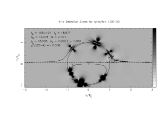
Figure 5: ${\Delta\chi^{2}}$ -vs- planet position for the data on 98BLG42. The black zones show where the presence of a planet with $q=10^{-3}$ is ruled out by our observations.

The probability of finding a planet on position $x,y$ on the lens plane given its orbital radius $a$ (assuming a randomly oriented circular orbit) is given by:

$$P(det|a)=\int P(det|x,y)P(x,y|a)dxdy.$$ (3)

The first term

$$P(det|x,y)=1-\exp{\left(\frac{-\Delta\chi^{2}(x,y)}{2}\right)}$$ (4)

is 0 in the ‘grey zones’ on Fig. 5, where a planet has no effect on the lightcurve, and 1 in the ‘black zones’, where the planet produces a large effect near one of the data points. This detection probability is appreciable only when the planet position $x,y$ is close to one of the images of the source at the time of one of the data points in the lightcurve. The interesting shape of the black zones in which the planet can be detected is due to details of lensing by two point masses, which we have calculated using the techniques of Gould and Loeb (1992).

The second term $P(x,y|a)$ is obtained by randomly orienting the planet’s assumed circular orbit of radius $a$, and then projecting it onto the $x,y$ plane of the sky. This gives a circular distribution centred on the lens star and rising as $(r/a)^{2}$ to a sharp peak at $r=a$, outside which the probability vanishes. This term may be written as:

$$P(x,y|a)=\frac{1}{2\pi a\sqrt{a^{2}-x^{2}-y^{2}}}$$ (5)

for ${r^{2}=x^{2}+y^{2}<a^{2}}$. A slightly elliptical orbit would blur out the outer edge, and it’s obviously possible to calculate this for any assumption about the eccentricity.

The net detection probability $P(det|a)$ is therefore the result of summing up the fraction of the time that a planet in the orbit of radius $a$ would be located inside one of the ‘black zones’ of Fig. 5. The result is plotted in Fig. 6. Since the detection zones are near the lens star’s Einstein ring, the detection probability is highest for planets with $a\sim R_{E}$.

Our observations, primarily the data points on 4 consecutive nights while the source was strongly amplified, yield a detection probability of about 10% for $a=R_{E}$. This detection probability is for a planet with a Jupiter-like mass ratio, $q=m_{p}/M_{L}=10^{-3}$, and for other planet masses it scales roughly as $\sqrt{q}$. For $a<R_{E}$ the detection probability in Fig. 6 is lower because the planet spends more of its time inside the detection zones. Discrete steps occur as the orbit radius shrinks inside each of the data points. For $a>R_{E}$ the planet spends most of its time outside the detection zones and the probability drops off as $(R_{E}/a)^{2}$.

Figure 6: The probability of detecting a planet with mass ratio q=$10^{-3}$ in orbit at radius $\alpha$ in units of the Einstein ring radius based on the observations for 98BLG42. The solid horizontal line indicates the total detection probability. The probability is maximized for orbital radius ${a/R_{E}\sim 1}$.

To summarize, our measurements of the lightcurve of 98BLG42 probe a substantial fraction of the lensing zone for the presence of Jupiters. Our detection probability, arising mainly from data on 4 consecutive nights of high amplification, is 10% for a planet with a Jupiter-like mass ratio $q=10^{-3}$ and orbit radius $a\sim R_{E}$. The gaps between our detection zones indicate that denser temporal coverage would improve the result for this event by perhaps a factor of 3. For even denser sampling, however, the detection zones in Fig. 5 would begin to overlap, diminishing the added value of each new data point toward the objective of detecting Jupiters.

6 SIMULATED DETECTION OF A JUPITER

In this section we show explicitly how Jupiters can be detected in lightcurve data obtainable from a northern site. Our goal is not to characterize the planet, but rather to show that we can discover that a planet deviation has occured, based on the daily sampling and accuracy attainable from a northern site.

To make a reasonably realistic assumption of our ability to detect planets, we add several fake data points to our observed lightcurve of 98BLG42. These points fill in a 4-day gap in the actual observations during the decline from peak amplification. The fake data points include the effect of a Jupiter mass planet located at ${x/R_{E}=1.05}$, ${y/R_{E}=0.39}$, which amplifies the major image on one night only. The magnitudes reported in this section are starman instrumental magnitudes.

The fake data points were obtained by using the lightcurve magnitude value for that day with an added random scatter value (${\Delta magnitude}$) within the limits imposed by the noise model.

The new lightcurve, including the fake data points and the best-fit point-lens lightcurve, are shown in Fig. 8. The fake data points on the night most affected by the planet perturbation lie significantly above the fitted point-lens lightcurve, and these high points pull the fit up so that other points fall systematically below the predicted lightcurve. As a result, the best fit achieved by the point-lens no-planet model has a ${\chi^{2}/27=2.8}$ with 4 parameters fitted to 31 data points. The 4 parameters were adjusted using the downhill simplex algorithm to minimize ${\chi^{2}}$ and were, namely, the time of maximum amplification, event timescale, maximum amplification and baseline magnitude (${t_{0},t_{E},A_{0},I_{0}}$ respectively).

The ${\chi^{2}}$ improves by a factor of 8, to ${\chi^{2}/27=0.35}$ for a star+planet lens model, as shown in Fig. 10. In this fit we adopt a planet/star mass ratio $q=10^{-3}$, and allow the planet to be anywhere on the plane of the sky, thus optimizing 2 additional parameters. This highly significant improvement in the fit is sufficient to reject the no-planet model in favor of the star+planet model. This can also be seen clearly on the residual patterns for both fits as illustrated in figures 8 and 10 for the no planet and planet fit respectively. The planet’s presence is thus detectable in the lightcurve.

Fig. 11 shows the ${\Delta\chi^{2}}$ map as a function of assumed planet position. Although the planet is detected, its mass and location are not well defined from the data. The data points that detect significant deviation from the point-lens lightcurve do not reveal the duration or shape of the planetary deviation. The planet could be interacting with either the major or minor images of the source star, and therefore could be located on either of several positions indicated by the white regions on Fig. 11. Thus while the planet is detected, it is certainly not characterized. Characterization obviously requires significantly more data points to record the shape of the planetary deviation.

Figure 7: Shown above is the best fit single lens model for a simulated lightcurve which includes a planetary deviation. The fitted parameters appear in the top left corner of the plot. The residuals of the fit are shown in fig 8. The ${\chi^{2}}$ value improves by a factor of 8 if we allow for the presence of a planet as shown in fig 10.

Figure 8: Fit residuals for the best single lens model fit as shown is fig 8.

Figure 9: Best fit lens+planet model for a simulated lightcurve which includes a planetary deviation. This gives a lower ${\chi^{2}}$ than figure 8, indicating a better fit. The fitted parameters appear in the top left corner of the plot and the planet is at position ${x/R_{E}=1.05}$, ${y/R_{E}=0.39}$ on the lens plane interfering with one of the major images.

Figure 10: Fit residuals for the fit including the planet in fig 10.

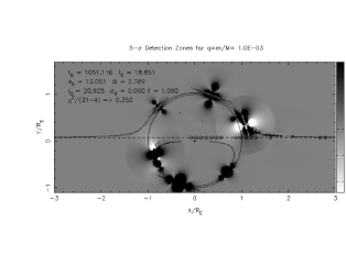
Figure 11: The dark zones on the $\chi^{2}$ map mark where the planets with $q=10^{-3}$ are excluded at the 5$\sigma$ level based on the simulated observations. White zones represent a successful detection. The planet is successfully detected at position ${x/R_{E}=1.05}$, ${y/R_{E}=0.39}$ on the lens plane where it interferes with one of the major images. Note that white detection zones also exist close to the minor image as well. This is because poor sampling cannot tell us exactly which image the planet is interacting with so we get white spots at both possible positions. This discrepancy can be solved if the sampling is sufficient to resolve the structure of the planet lensing event in detail.

Since up to now there have been no confirmed reports of any planetary deviations by any microlensing follow-up network, it is our belief that nightly monitoring schemes, taking a couple of exposures per night for a number of events (as suggested in section 2) might yield the first detections. Even more so if numerous telescopes contribute observations to the effort and data are shared in a common database.

7 CONCLUSION

We have used 1 hour per night on the IAC 0.8m telescope in Tenerife for CCD monitoring of the lightcurves of Galactic Bulge microlensing events during the 1998 season. The best observed event in our dataset is 98BLG42, for which we obtain accurate measurements on 4 consecutive nights beginning just before the peak of the event, and lower accuracy measurements in the tail of the event. Our data are consistent with a point lens lightcurve. We identify the detection zones near the Einstein ring of the lens star where our data rule out the presence of a planet with a Jupiter-like planet/star mass ratio $q=10^{-3}$. For such planets our detection probability is 10% for orbit radius $a\sim R_{E}$, falling off for larger and smaller orbits.

We also demonstrate explicitly, by adding a few fake data points to our actual CCD data, the feasibility of detecting planets by monitoring microlensing lightcurves from small (1m) telescopes at northern sites, despite the degradation of accuracy arising from poorer seeing at higher airmass.

If such an observing scheme is to be pursued, ongoing events could be preselected from the alerts issued by the detection teams (OGLE, EROS) and observations could be directed to those of high amplification since the signal-to-noise (S/N) achieved should be better for those. Dense sampling should be dedicated to clearly defining the primary peak and probing for secondary peaks in this region. If the lensing star has a planetary companion, the probability of detecting it is highest if the planet has an orbital radius ${a\simeq R_{E}}$, the Einstein ring radius. In this case the planet could be perturbing either the minor or the major image, which are located respectively just inside or just outside the Einstein ring at the high amplification part. Since the detection probability is much lower for ${a>>R_{E}}$ the event need not be monitored as densely for amplifications less than 1.34, where only a few data points are needed to establish the baseline level. The possibility of making observations from northern sites may also yield crucial data points on events that cannot be followed during certain times from southern sites where most teams currently operate.

8 ACKNOWLEDGEMENTS

The data reductions were carried out at the St.Andrews node of the PPARC Starlink Project. RAS was funded by a PPARC research studentship during the course of this work. The IAC80 telescope is operated at Izana Observatory, Tenerife by the Instituto de Astrofysica de Canarias.

References

- [\citefmtAlard & Lupton1998] Alard C., Lupton R., 1998, ApJ, 503, 325
- [\citefmtAlbrow et al.1998] Albrow M. et al., 1998, ApJ, 509, 687
- [\citefmtAlcock et al1997] Alcock et al C., 1997, ApJ, 479, 119
- [\citefmtBennet & Rhie1996] Bennet D., Rhie S., 1996, ApJ, 472, 660
- [\citefmtGould & Loeb1992] Gould A., Loeb A., 1992, ApJ, 396, 104
- [\citefmtMarcy & Butler1996] Marcy G., Butler R., 1996, ApJ, 464, 147
- [\citefmtPaczynski1986] Paczynski B., 1986, ApJ, 304, 1
- [\citefmtPaczynski1996] Paczynski B., 1996, ARA&A, 34, 419
- [\citefmtPenny1995] Penny A., 1995, Starlink User Note 141.2, Rutherford Appleton Laboratory
- [\citefmtRhie & Bennet1998] Rhie S., Bennet D., 1998, 193,
- [\citefmtUdalski et al1994] Udalski et al A., 1994, ApJ, 436, L103
- [\citefmtWolzczan & Frail1992] Wolzczan A., Frail D., 1992, Nat, 355, 145