The SZ effect as a cosmological discriminator

Abstract

We show how future measurements of the SZ effect (SZE) can be used to constrain the cosmological parameters. We combine the SZ information expected from the Planck full-sky survey, $N(S)$, where no redshift information is included, with the $N(z)$ obtained from an optically-identified SZ-selected survey covering less than $1$ % of the sky. We demonstrate how with a small subsample ($\approx 300$ clusters) of the whole SZ catalogue observed optically it is possible to drastically reduce the degeneracy among the cosmological parameters. We have studied the requirements for performing the optical follow-up and we show the feasibility of such a project.
Finally we have compared the cluster expectations for Planck with those expected for Newton-XMM during their lifetimes. It is shown that, due to its larger sky coverage, Planck will detect a factor $\sim 5$ times more clusters than Newton-XMM and also with a larger redshift coverage.

1 Introduction

Clusters of galaxies have been widely used as cosmological probes. Their modeling can be easily understood as they are the final stage of the linearly evolved primordial density fluctuations (Press & Schechter 1974, hereafter PS). As a consequence, it is possible to describe, as a function of the cosmological model, the distribution of clusters and their evolution, the mass function, which is usually used as a cosmological test (Bahcall & Cen 1993, Carlberg et al. 1997, Bahcal & Fan 1998, Girardi et al. 1998, Rahman & Shandarin 2000, Diego et al. 2000) Therefore, a detailed study of the cluster mass function will provide us with useful information about the underlying cosmology.
Following this idea, several groups have tried to constrain the cosmology by using the information contained in the mass function. They compare the observational mass function with the theoretical one given by the PS formalism (Carlberg et al. 1997, Bahcall & Fan 1998) or with simulated ones from N-body simulations (Bahcall & Cen 1993, Bode et al. 2000). The method has shown to be very useful but it is limitted by the quality of the data. Cluster masses are not very well determined for intermediate-high redshift clusters and even for low redshift ones the error bars are still significant. The standard methods to determine cluster masses (velocity dispersions, cluster richness, lensing, X-ray surface brightness deprojection) usually give different answers. It is believed that the best mass estimator is the one based on lensing (e.g. Wu & Fang 1997, Allen 1998) but the number of clusters with masses measured with this technique is too low to make this method a reliable technique to build a statistically complete mass function although several attempts have been made (Dahle 2000).
Instead of the mass function, it is possible to study the cluster population through other functions like the X-ray flux or luminosity functions or the temperature function. The advantage of these functions compared with the mass function is that in these cases the estimation of the X-ray fluxes, luminosities, or temperatures of the clusters is less affected by systematics than the mass estimation from optical data. The drawback, however, is that to build these functions from the mass function, a relation between the mass and the X-ray luminosity, or flux or temperature is needed. These relations are known to suffer from important uncertainties which should be taken into account. These uncertainties have their origin in the intrinsic scatter of these relations as well as in the quality of the observational data used to build them.
There are three basic wavebands in which galaxy clusters are observed; optical (galaxies bounded to the cluster), X-ray (bremstrahlung emission from the very hot intra-cluster gas), and more recently in the mm waveband (Sunyaev-Zeldovich effect, SZE).
The first clusters were observed with optical telescopes and also the first cluster catalogues were based on optical observations (Abell 1958; Abell, Corwin & Olowin (ACO) 1989; Lumsden et al. 1992 (EDCC); Postman et al. 1996 (PDCS); Carlberg et al. 1997b (CNOC)). However the optical identification of a cluster is not a trivial task. First, it is not easy to define the cluster limits or cluster size. When observed in the optical band, a cluster appears as a group of galaxies which are bounded by the common gravitational potential. However, in the outer parts of the cluster there can be some galaxies for which it is not clear to what extent they are bounded to the cluster or, on the contrary, they are field galaxies.
Optical identification of clusters has other more important shortcomings. They specially suffer from projection effects, that is, there can be some galaxies in the line of sight which are not bounded by any gravitational force but they can appear as a bounded system because their images are projected onto a small circle centered on the cluster position. The best way to reduce this effect is by means of spectral identification. However, these kind of observations are time consuming and, when observing distant clusters, spectral identification is only feasible for the most luminous galaxies in the cluster.

These problems are reduced when the cluster is observed in the X-ray band. In this band clusters appear as luminous sources due basically to the continuos bremstrahlung emission coming from the very hot ($T\sim 10^{7}$ K) intracluster gas. The same intracluster emission can be used to determine the cluster gas size. Moreover, projection effects are weaker in this case, thus X-ray surveys are very efficient in detecting clusters. However, with X-ray surveys it is difficult to detect clusters further than $z\approx 1$. There are two reasons for this. One lies in the fact that the X-ray cluster emissivity is proportional to $n_{e}^{2}$ where $n_{e}$ is the electron density, that is, the emissivity drops very fast from the center of the cluster to the border and only the most dense central parts of the cluster will originate a substantial X-ray emission. This makes very difficult the detection of distant clusters for which the X-ray emission is concentrated in the central parts of the cluster and therefore the apparent angular size will be very small. Moreover the X-ray flux declines as $D_{L}^{-2}=(D_{m}(1+z))^{-2}$ ($D_{m}$ is the comoving distance and $D_{L}$ the luminosity distance). This selection function limits the redshift at which one cluster can be observed by actual X-ray detectors which are blind to the earlier stages of cluster formation ($z\ga 2$).

In the mm waveband the situation is quite different. The SZE surface brightness goes as $n_{e}$. Therefore, when observing the clusters at mm wavelengths, it would be easier to detect the most distant ones because they will show a larger apparent angular size since the brightness profile drops more slowly than in the X-ray case. In X-rays, the total flux decays as $D_{L}^{-2}$. Meanwhile, the integrated SZE flux goes as $D_{a}^{-2}=(D_{m}/(1+z))^{-2}$ ($D_{a}$ being the angular diameter distance). $D_{a}$ grows more slowly than $D_{L}$ and even decreases after a certain redshift $z\approx 1$. Therefore, the SZE flux drops more slowly with distance (or even increases) in the case of the SZE than in the X-rays case. Another advantage is that, as in the X-ray situation, galaxy clusters observed through the SZE does not suffer (almost) from projection effects. All these reasons make the SZE the preferable way of observing distant clusters.

Our interest on the SZE is twofold. First, it can be considered as a contaminant of the cosmological signal (CMB) and therefore a good knowledge of this effect is required in order to perform an appropriate analysis of the CMB data. But it can also be considered as a very sensitive tool to measure the mass-space cluster distribution. In this paper we will concentrate our effort in this second aspect.
Planned CMB surveys will also be sensitive to the SZE distortion induced by galaxy clusters (MAP, Planck). These surveys will cover a wide area of the sky and they are expected to detect the SZE signature for thousands of clusters. Furthermore, proposed and undergoing mm experiments will measure the SZE for hundreds of clusters in the near future (e.g. AmiBa, Lo et al. 2000; LMT-BOLOCAM, López-Cruz & Gaztañaga 2000; CBI, Udomprasert et al. 2000; AMI, Kneissl et al. 2001; or the interferometer proposed in Holder et al. 2000) The cosmological possibilities of these new data sets are very relevant as they will have a statistically large number of clusters and they will improve the redshift coverage significantly. For a realistic prediction of the power of future SZE surveys we should consider the detector characteristics of one of these planned experiments. In this work we will focus our attention on the expected SZE detections for the Planck mission and we will study the possibilities of these data to probe the cosmological model. Planck will observe the whole sky at 9 mm frequencies (including those where the SZE is more relevant) and with angular resolutions ranging from 5 arcmin to 33 arcmin FWHM (see fig. 1 below). The observation of the SZE at different frequencies will make easier the task of identifying clusters because of the peculiar spectral behaviour of the SZE signal which can be very well recognized with the nine Planck frequencies. As can be seen from figure (1), the best channels are the ones at 100 GHz ($x=1.76$), 143 GHz ($x=2.5$) and 353 GHz ($x=6.2$) together with the channel at 217 GHz ($x=3.8$) where the thermal SZE vanishes. A cross correlation of these channels, including the knowledge of the spectral shape factor, will allow to discriminate among the SZE, foregrounds and CMB.

As we will show in the next sections, the cluster population at high redshift is much more sensitive to the cosmological parameters than the cluster population in the local Universe ($z\la 0.5$). Thus, the information at high redshift is crucial to determine the underlying cosmology and the SZE can be the tool to get that information.

The structure of this paper is the following; in section 2 we recall some of the basics of the SZE and some useful definitions which will be of interest in subsequent sections. In section 3, we show how through the SZE we can investigate the cluster population and evolution. We also show in section 4 how future SZE surveys should be complemented with optical observations of a small subsample of SZE-selected clusters in order to provide redshift information of those clusters; in this way, it is possible to reduce the degeneracy in the cosmological models describing the data. We apply this idea in section 5 to simulated Planck SZ data. In that section we obtain some interesting results about the possibilities of those future data. Finally we discuss our results and we conclude in section 6.

2 The Sunyaev-Zel‘dovich effect

Since Sunyaev & Zel’dovich predicted that clusters would distort the spectrum of CMB photons when they cross a galaxy cluster (Sunyaev & Zel’dovich 1972), several detections of this effect have been made. At present, the number of clusters with measured SZE is small because they are limitted by the detector sensitivity (a typical SZE signal is of the order of $10^{-4}$ in $\Delta T/T$ with $\bar{T}\approx 2.73$ K). However, the sensitivity in the detectors is getting better and better and in a few years the number of detected clusters through the SZE will make this effect an important tool to explore clusters at high redshift.

When CMB photons cross a cluster of galaxies, the spectrum suffers a distortion due to inverse Compton scattering. The net distortion in a given direction can be quantified by the cluster Comptonization parameter, $y_{c}$, which is defined as

$$y_{c}=\frac{\sigma_{T}k_{B}}{m_{e}c^{2}}\int Tn_{e}(l)dl.$$ (1)

The integral is performed along the line of sight through the cluster. $T$ and $n_{e}$ are the intracluster electron temperature and density respectively; $\sigma_{T}$ is the Thomson cross section which is the appropriate cross section in this energy regime and $k_{B}$ is the Boltzmann constant.
The flux and the temperature distortion are more widely used than the Compton parameter because these are the quantities which are directly determined in any experiment when observing clusters at mm frequencies. The distortion in the background temperature is given by:

$$\frac{\delta T}{T}=g(x)y_{c}\ ,$$ (2)

where $x=h\nu/kT_{CMB}$ is the frequency in dimensionless units and $g(x)=xcoth(x/2)-4$ is the spectral shape factor. There is a second kind of distortion due to the bulk velocity of the cluster. It is known as the kinetic SZE. However, this contribution is much smaller than the thermal contribution and we will not consider that in this work.
As can be seen from the previous equation, there is no redshift dependence on the temperature distortion, i.e, the same cluster will induce the same distortion in the CMB temperature, independently of the cluster distance (except for relativistic corrections). The only redshift dependence of the total SZE flux is due to the fact that the apparent size of the cluster changes with redshift.
The total SZ flux is given by the integral :

$$S_{total}(\nu)=\int_{cluster}\Delta I(\nu,\vec{\theta})d\Omega,$$ (3)

where the integral is performed over the solid angle subtended by the cluster. $\Delta I(\nu,\vec{\theta})$ is the change in intensity induced by the SZE and is given by $\Delta I(\nu,\vec{\theta})=I_{0}f(x)y_{c}$ where $I_{0}=(2h/c^{2})(k_{B}T_{CMB}/h)^{3}$ and

$$f(x)=\frac{x^{4}e^{x}}{(e^{x}-1)^{2}}\left[\frac{x(e^{x}+1)}{(e^{x}-1)}-4\right],$$ (4)

is the spectral shape (see fig.1).

Figure 1: Spectral shape of the thermal SZE. Planck channels are between $30$ GHz and $800$ GHz (black dots), including also the $217$ GHz channel where the thermal SZE vanishes. The best channels to detect the SZE decrement/increment will be those of the HFI instrument at 100 GHz ($x=1.7$), 143 GHz ($x=2.5$) and 353 GHz ($x=6.2$) respectively together with the one at 217 GHz ($x=3.8$). At 100 GHz ($x=1.7$) there are two channels: the LFI (solid line) and the HFI (dotted line).

In fig. 1 we show the spectral shape of the SZE $f(x)$. In the same plot the 9 frequency channels from Planck are shown as black dots. The amplitude of the lines are proportional to the SNR per resolution element in each channel (assuming that the clusters are unresolved). The SNR depends on the spectral shape factor $f(x)$ since the signal is proportional to $f(x)$ (see eq. 5 below) and the sensitivity per resolution element ($\sigma$); $SNR=S/N\propto f(x)/\sigma$ which is proportional to the amplitudes represented in fig. 1.

Eq. (3) can be easily integrated assuming that the cluster is isothermal. Then the integral can be reduced to $\propto\int d\Omega\int n_{e}(\vec{\theta})d\ell$ which can also be transformed into $D_{a}^{-2}(z)\int dVn_{e}(\vec{\theta})=D_{a}^{-2}(z)\frac{M_{gas}}{m_{p}}=D_{a}^{-2}(z)\frac{f_{b}}{m_{p}}M$. $M$, $f_{b}$ and $m_{p}$ are the total mass, baryon fraction and the proton mass respectively. In this approach, we have assumed that the gas is only composed of ionized Hydrogen. Finally we get:

$$S_{SZE}=\frac{3.781f(x)f_{b}TM_{15}}{D_{a}^{2}(z)}.$$ (5)

In the previous expression $T$ is given in Kelvin, $M_{15}$ in $10^{15}M_{\odot}$ and $D_{a}(z)$ in Mpc. In these units, the flux is given in mJy (1 mJy = $1.0\times 10^{-26}$ erg s^-1 Hz^-1 cm^-2). If we now introduce the $h$ dependency in $M_{15}$ ($10^{15}h^{-1}M_{\odot}$), $D_{a}(z)$ ($h^{-1}$ Mpc) and $f_{b}\approx 0.06h^{-1}$ then the flux is given also in mJy units.

Eq. (5) tell us that the total flux is given basically by three terms: temperature, mass and angular-diameter distance to the cluster. As a difference with the X-ray flux, where in the integral over the cluster volume one should consider $n_{e}^{2}$ instead of just $n_{e}$, the total SZE flux does not depend on the cluster profile. Therefore, for an isothermal cluster, no assumption about the electron density profile is needed when computing the total SZE flux. This aspect is very important since for the Planck resolution, only a small percentage of the clusters ($\approx$ 1 %) will be resolved and as a first approximation we can consider that all the fluxes can be computed from eq. (5). This fact will simplify significantly our calculations and simultaneously will reduce the uncertainty due to the lack of a precise knowledge of the cluster density profile.
The second important consequence that we can remark from the previous equation is about the angular-diameter distance dependence of the total flux. In X-rays, the total flux depends on $D_{L}^{-2}(z)$. If we compute the ratio $D_{a}^{2}(z)/D_{L}^{2}(z)$ it goes like $(1+z)^{-4}$, that is, the $S_{SZE}$ drops a factor $(1+z)^{-4}$ slower than the $S_{X}$. Thus for high redshift clusters it is evident the advantage of using mm surveys (SZE) as compared with the X-ray ones.

If the cluster is unresolved by the antenna, then the cluster total flux (eq. 5) can be considered contained in the resolution element of our antenna. If on the contrary, the cluster is resolved, then the previous approximation is not adequate anymore and we should integrate the surface brightness over the cluster solid angle.
The gas density profile can be well fitted by a $\beta$-model.

$$n_{e}(r)=n_{o}(1+(r/r_{c})^{2})^{-3\beta/2},$$ (6)

where $n_{o}$ is the central electron density ($n_{o}\approx 2.0\times 10^{-3}(1+z)^{3}h^{1/2}e^{-}/cm^{3}$) and $r_{c}$ is the core radius of the cluster. The observed values of $\beta$, obtained from X-ray surface brightness profiles, typically range from 0.5 to 0.7 (Jones & Forman 1984, Markevitch et al. 1998).

3 SZE as a probe of the cosmological model

As we mentioned in the introduction, an estimate of the cluster mass function can be used to constrain the cosmological parameters. However such estimate is affected by the systematics in the mass estimators. It is possible to use other functions to explore the cluster population like for instance the temperature function $d^{2}N/dTdz$ (Henry & Arnaud 1991, Eke et al. 1998, Viana & Liddle 1999, Donahue & Voit 1999, Blanchard et al. 2000, Henry 2000). The connection between the mass function and the temperature function is the $T-M$ relation,

$$\frac{d^{2}N}{dTdz}=\frac{d^{2}N}{dMdz}\frac{dM}{dT}$$ (7)

Temperature estimates are more reliable than mass estimates. Therefore the temperature function should be less affected by the systematics than the mass function. However, the scatter in the $T-M$ relation introduces new uncertainties which should be taken into account. Similar problems have the X-ray luminosity function and the X-ray flux function which have been widely used in the literature to constrain the cosmological parameters (Mathiesen & Evrard 1998, Borgani et al. 1999, Diego et al. 2000). In those cases new uncertainties appear due to the scatter in the $L_{x}-T$ relation. In a previous work (Diego et al. 2000), we have considered these ideas and applied them to constrain the cosmological parameters by fitting the model to different data sets: mass function, temperature function, X-ray luminosity and flux functions. That work was innovative in the sense that we considered all the previous data sets simultaneously in our fit (and not just one as usual) and we looked for the best fitting model to all the data sets considered. Also important is to remark that in that work we considered the cluster scaling relations as free-parameter relations. These two points are very relevant because when fitting cluster data sets it is important to check that the best fitting models agree well with other data sets. Otherwise, we should reexamine the assumptions made in the model. One of these assumptions is, for instance, the cluster scaling relations $T-M$ or $L_{x}-T$. These relations are commonly fixed a priori. However they are known to suffer from important scatter as we have shown in that work. In fact, we found that not all the scaling relations considered previously in other works were appropriate to describe conveniently several cluster data sets in a simultaneous fit. By fitting our free-parameter model to all the data sets, we obtained, not only the cosmological parameters, but also the best scaling parameters. In that work we found as our best fitting parameters the ones given in table 1.

Table 1: Best $\Lambda$CDM (flat) and OCDM ($\Lambda=0$) models. Both models are undistinguishable in the redshift regime of the data considered in Diego et al. (2000).

Model	$\sigma_{8}$	$\Gamma$	$\Omega_{m}$	$T_{0}(10^{8}h^{\alpha}K)$	$\alpha$	$\psi$
$\Lambda$CDM	0.8	0.2	0.3	1.1	0.75	1.0
OCDM	0.8	0.2	0.3	1.1	0.8	1.0

The first 3 columns correspond to the cosmological parameters and the others are for the $T-M$ relation;

$$T_{gas}=T_{0}M_{15}^{\alpha}(1+z)^{\psi},$$ (8)

where $M_{15}$ is the cluster mass in $10^{15}h^{-1}M_{\odot}$ and $T_{0}$, $\alpha$, and $\psi$ were free parameters. We found that the two models in table 1 were undistinguishable when they were compared with the data. In fact, both models agree well with the data considered and there was no way to determine which one was the best. In order to distinguish them, more and better quality data are needed. Undergoing X-ray experiments (CHANDRA, Newton-XMM) will help to do that as well as current and proposed optical surveys (e.g. Gladders et al. 2000). The models which were undistinguishable in the low redshift interval will show different behaviour at higher redshift. However, as we mentioned in the introduction, the waveband in which distant clusters will be detected the most, is not the optical nor the X-ray band, but the mm band. The usefulness of the SZE as a tool to measure cosmological parameters motivated many works in the past (e.g. Silk & White 1978, Markevitch et al. 1994, Bartlett & Silk 1994, Barbosa et al. 1996, Aghanim et al. 1997) as well as in the present time (Holder et al. 2000, Grego et al. 2000, Mason et al. 2001, this work).

Using SZ data it is possible to estimate the cosmological parameters by looking at some SZ derived function related with the mass function. We just need a measurement of a cluster quantity related with its mass. As we have shown in eq. (5), the total SZ flux can be such a quantity. From that equation it is possible to build a mm flux function ($dN/dS_{mm}$) from a mass function ($dN/dM$). An interesting alternative to this approach can be found in Xue & Wu (2001). In that paper the authors have connected the mm flux function with the observed X-ray luminosity function through the $L_{x}-T$ and $T-M$ relations. If we consider a future mm experiment (like Planck) where thousands of clusters are expected to be detected through the SZE, probably a fit to the mm flux function could be able to distinguish the models in table 1. In fig. 2 we show the expected number of clusters with total flux above a given flux for the two previous models. These are integrated fluxes, i.e we assume that the clusters are not resolved and that their total flux falls into the antenna beam size. This assumption is appropriate when the antenna size is above several arcmin as it is the case for the Planck satellite where its best resolution is FWHM = $5$ arcmin.
In fig. 2 we did not show the whole ($0<z<\infty$) integrated $N(>S)$ curve since it looks quite similar to the two curves on the top of the figure and they still look undistinguishable. To compare them in a more realistic way we have performed a Kolgomorov-Smirnov test where we have compared the $N(>S)$ curve for a realization (over 2/3 of the sky) of the $\Lambda$CDM model with the mean expected values of both OCDM and $\Lambda$CDM models. The KS test was unable to distinguish between the models.

Figure 2: The SZE integrated number counts of the cluster population predicted at mm wavelengths (353 GHz) for the best flat (solid) and open (dotted) models in table 1. In the plot three redshift shells are represented: top $z<1$, middle $z\in[1,2]$ and bottom $z>2$.

As can be seen from the figure, both models predict the same number of clusters in the $z<1$ redshift interval (top). That situation was similar in Diego et al. (2000) where most of the cluster data were at low $z$ and it was not possible to discriminate between both models.
But the situation changes at redshifts $z>1$. In the redshift bin $z\in(1,2)$ (middle) the differences between both models are significant. These differences are increased when we compare the models in the redshift bin $z>2$ (bottom) where in the OCDM model two orders of magnitude more clusters are expected than in the $\Lambda$CDM case above $S=30$ mJy. This flux ($S=30$ mJy at 353 GHz) is expected to be the flux limit of Planck (see Appendix A where we estimate that limit based on MEM residuals). However, this limiting flux will depend on the method used to identify such clusters in the maps. The final method to be used with Planck is still under development. MEM methods work very well (Hobson et al. 1998, Hobson et al. 1999) being at present the preferred one.
In fig. 3 we show the number of clusters with fluxes above that limiting flux of Planck as a function of redshift. Again the differences are not significant below $z\approx 1$ but they are quite relevant above that redshift. By looking at figs. (2) (3), we see that the differences in the cosmological models are more evident at high redshift. In order to discriminate among the cosmological models one should consider not only the cluster population at low redshift (normalization) but the cluster population at high redshift (evolution) as well. A recent application of this idea can be found in Fan & Chiueh (2000) where the authors study the function $r=N(z<0.5)/N(z>1)$ as a function of the limiting flux. That work suggests that a limitted knowledge of the redshift of the cluster would allow to constrain the cosmological parameters.

Figure 3: The SZE differential number counts of the cluster population predicted for the Planck mission at mm wavelengths (353 GHz) for the best flat (solid) and open (dotted) models in table 1 as a function of redshift.

Both fig. 2 and fig. 3 suggest that with future SZE data it will be possible to go further on the determination of the cosmological parameters. From all these plots, it is evident that Planck (together with redshift information for a small subsample, see next section) would be able to discriminate between the models which previously were undistinguishable when they were compared with present X-ray and optical data. Furthermore, the accuracy in the free parameters obtained in previous works will be increased with these new data.

3.1 Montecarlo simulations: Planck vs Newton-XMM

The previous discussion was based on theoretical expectations of the mean number of SZE detections expected at different redshifts. We want to go further by computing Montecarlo (Press-Schechter) realizations of the expected SZE on a specific patch of the sky. In order to compare the mm and X-ray bands we will also compare the expected SZ detections in this area for Planck with those based on X-ray expectations for Newton-XMM in the same sky patch.

The simulations were done over a patch of the sky of $12.8^{\circ}\times 12.8^{\circ}$ and with a pixel size of $1.5^{\prime}\times 1.5^{\prime}$ filtered with a FWHM of $5$ arcmin and at the frequency of 353 GHz, following the characteristics of the 353 GHz channel of Planck.
The parameters of this simulation corresponds to the $\Lambda$CDM model of table 1.

The total number of clusters is about $\approx 20000$ in one of these simulations. The mean Comptonization parameter is well below the FIRAS limit ($\sim 10^{-6}$ compared with $2.5\times 10^{-5}$, Fixsen et al. 1996). The resulting distribution of clusters is shown in figure 4. The allowed range of simulated masses was $3.0\times 10^{13}h^{-1}M_{\odot}<M<1.0\times 10^{16}h^{-1}M_{\odot}$. The lower limit is at the frontier between a small cluster and a galaxy group and it is the mass corresponding to a cluster with temperature $T\sim 1$ keV which can be considered as the minimum temperature for a virialized cluster.
In fig. 4 each point corresponds to one cluster with mass $M$ and redshift $z$. This distribution is in agreement with the observational constraint given by the detection of at least three clusters with masses above $0.8\times 10^{15}M_{\odot}$ and $z>0.5$ (Bahcall et al. 1998).
The most massive cluster is at redshift 0.66 with a mass $M=1.09\times 10^{15}h^{-1}M_{\odot}$ although this was an unusual realization. In a normal one of this size, the most massive cluster is usually well below $z\approx 0.5$. Clusters marked with an open circle correspond to those with a total flux above $30$ mJy and according to our criterion, these clusters would be detected by Planck (see Appendix A). There are 185 clusters above this limit and only one of them would be observed above $z=1$ in this simulation. As a comparison we show the same picture but corresponding to the OCDM model in table 1. (fig. 5). In this case $\approx 15$ clusters are detected above redshift $z=1$. This comparison demonstrates how a small region of the sky can show up the differences between the two models in table 1. Both models are nearly undistinguishable below $z\approx 0.7$ but they differ significantly above that redshift. We will come later to this point in section 4.

As a comparison with the number of detected clusters expected with Planck, we show in figs. 4 and 5 the clusters expected to be detected by Newton-XMM (big solid circles, $S_{X}>1.5\times 10^{-14}$ erg s^-1 cm^-2 in the $0.5-2$ keV band, Romer et al. 1999).
Solid lines represent the minimum mass as a function of redshift for which the corresponding flux is above the limiting flux in Planck and Newton-XMM respectively, that is, they are the selection functions for both missions.

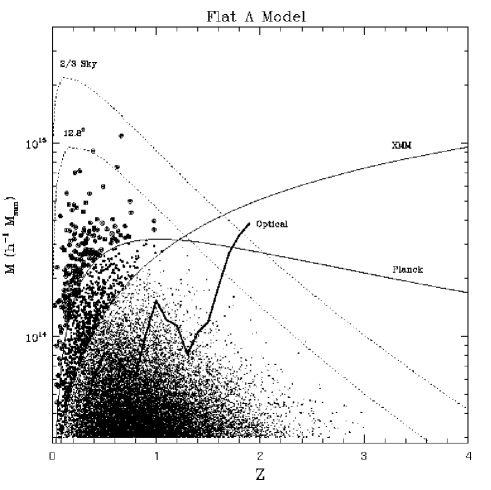
Figure 4: $\Lambda$CDM model. Each cluster is represented as a dot in this plot. Clusters marked with a big black dot have fluxes (in the $0.5-2$ keV band) above the limiting flux $S_{X}=1.4\times 10^{-14}$ erg s^-1 cm^-2 and they are the clusters expected to be detected by Newton-XMM in the XCS (Romer et al. 1999). Cluster marked with an open circle are those with a SZE flux above $30$ mJy at $353$ GHz and they are the clusters expected to be detected by Planck. Solid lines represent the masses for which the flux equals the limiting flux of Planck ($30$ mJy), and the XCS. Dotted lines show the maximum cluster mass expected in a solid angle equal to $2/3$ of the sky (top) and $(12.8^{\circ})^{2})$ (bottom). Finally the heavy solid line indicates the selection function for an hypothetical optical survey made with a 10-m class telescope and two hours of observation (8 bands and 900s per band. See section 4.1).

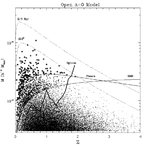
Figure 5: OCDM case. Note the differences in the cluster distribution above the coasting phase redshift $z_{c}\approx 0.7$ (see text).

Although Newton-XMM will see many more clusters at low redshift, however Planck will be more sensitive to those clusters at high redshift. The reason is that the corresponding selection functions are different in both cases. The X-ray flux goes as $S_{X}\propto D_{L}^{-2}(z)$ and to detect clusters deeper in redshift they must be more luminous (more massive) in order to compensate the monotonous increasing function $D_{L}(z)$. On the contrary, the SZE flux goes like $S_{SZE}\propto D_{a}^{-2}(z)$ and at redshift $\approx 1$, the angular diameter distance reaches a maximum and after that it starts to drop to smaller values. Therefore the masses needed to provide a particular flux, $S_{SZE}=30$ mJy, can be smaller at redshift $z>1$ than the required masses at $z\approx 1$.
The dotted lines in figs. (4) and (5) indicate the maximum expected mass as a function of redshift in the simulation for the specific solid angle $2/3$ of the sky (top) and $12.8^{2}deg^{2}$ (bottom). The point where the selection function cross these maximum mass lines corresponds to the maximum redshift expected in the sample. In both cases, Planck goes deeper than Newton-XMM. The difference can be even more emphasized if the limiting flux for Planck is below the one considered in this paper which was a very conservative one (see Appendix A).

As noted in Romer et al. (1999), the XMM Cluster Survey (XCS) will cover $\sim 800$ square degree and will contain more than $8000$ clusters. On the contrary Planck will observe the full sky, that is the sky coverage will be $\approx 50$ times larger than that of the XCS. In order to compare Newton-XMM with Planck this difference in the sky coverage should be considered. In fig. 6 we show the number of detected clusters expected by Planck and Newton-XMM (XCS) where we have taken into account the sky coverages and limiting fluxes expected for both missions.

Figure 6: Expectations for Planck (solid line OCDM, dotted line $\Lambda$CDM) and the XCS (dot-dashed line OCDM, dashed line $\Lambda$CDM).

Now, the differences between Planck and Newton-XMM are evident. The large sky coverage of Planck together with the constancy of the SZE surface brightness with redshift, will allow this satellite to detect a much more significant number of clusters than Newton-XMM in the XCS. Also, we can conclude from this plot that, for the best fitting models in table 1, no clusters are expected to be detected above $z\approx 3$, neither for the OCDM nor the $\Lambda$CDM. However the cluster abundance between $z=1$ and $z=2$ will provide a definitive probe of the cosmological parameters and the cluster scaling relations.

An important consequence of the previous plots (figs. 4 and 5) is that only a small portion of the whole sky would be needed to distinguish between the two models $\Lambda$CDM and the OCDM. This is an important point because only spectral identification of $\approx 200$ (not resolved) random selected clusters from the whole catalogue would be needed. However, it is important to answer the question, what is the minimum number of clusters needed to distinguish the models in table 1 at, for instance, the 3 $\sigma$ level? We will try to answer this question in the next section.

4 An optically-identified SZ-selected catalogue

As we have seen in fig. 2, the information provided by an hypothetical $N(S)$ curve (even if this curve corresponds to a full sky survey) will be insufficient to distinguish the two models considered in that figure. Redshift information will be needed in order to make the distinction. Different cosmological models predict different cluster populations as a function of redshift. If we analyze the evolution of the cluster population with $z$, then we should be able to discriminate among those models. However, to study the evolution of the cluster population we need spectral identification of the clusters (or at least optical observations in several bands in order to get photometric redshifts) since the SZE does not provide any estimate of $z$. Performing these observations for an hypothetical full sky SZ catalogue would be a huge task but if only a small number of unresolved clusters need to be identified then the work is significantly simplified. Now, we should ask the question, how small can our optically-identified sample be if we want to distinguish between, for instance, the two models in table 1? To answer that question we have compared the curves $N(S_{mm}>30$ mJy$,>z)$ for the two models in which we are interested. We require that at a given redshift, both curves must be distinguished at a $3\sigma$ level, that is, we require the condition $N^{O}-3\sqrt{N^{O}}=N^{\Lambda}+3\sqrt{N^{\Lambda}}$ (assuming Poissonian statistics), where $N^{O}$ and $N^{\Lambda}$ are the number of detected clusters above a given $z$ in the two cases OCDM and $\Lambda$CDM respectively.
Since we know $N^{O}$ and $N^{\Lambda}$ at each $z$, then we can compute the required total number of clusters which should be observed in order to satisfy the previous condition at each redshift. In fig 7 we show this calculation for three different selection criteria of the clusters. In each one of the lines we show the total number of clusters randomly selected from the catalogue (with the only condition that the total flux must be $S_{mm}>100$ mJy top, $S_{mm}>30$ mJy middle and $30$ mJy $<S_{mm}<40$ mJy bottom) which should be optically observed in order to distinguish (at a 3$\sigma$ level) $N^{O}$ and $N^{\Lambda}$ at redshift $z$ (i.e. the total number of observed clusters needed to have a $3\sigma$ difference in $N(>z)$ for the two models). As can be seen from the plot, randomly selecting about $300$ clusters with $S_{mm}>30$ mJy from the full catalogue and determining the redshift for each one, will allow to distinguish the two models at a 3$\sigma$ level above $z\approx 0.6$ just by looking at the $N(>z=0.6)$ curve. The explanation for this fact is given by the different evolution of the cluster formation in both models. In the $\Lambda$CDM case there is a coasting phase (or inflection point in the acceleration parameter) at $z_{c}\approx 0.7$ that helps to form structure at this redshift. This phase is not present in the OCDM case where there is a redshift $z_{c}\approx 2$ below which the collapse of linear fluctuations is inhibited by the fast expansion of the Universe.
Choosing the selection criteria $30$ mJy $<S_{mm}<40$ mJy, it is possible to reduce slightly the number of clusters to be identified. If on the contrary, only the brightest clusters with $S_{mm}>100$ mJy are identified optically, then we would need a significantly larger number of clusters in order to make the distinction between the models.

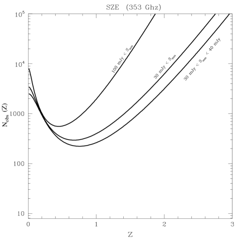
Figure 7: Required number of clusters to be observed in order to distinguish the OCDM and $\Lambda$CDM models.

4.1 Cluster optical detection simulations

Probably the most cost efficient way of identifying in the optical the galaxy clusters detected by Planck is using photometric redshifts. Even a rough estimate of the photo-z allows to considerably reduce the background galaxy contamination and enhance the contrast density of the cluster. In addition, although the error in the photo-z of an individual galaxy is usually $\approx 0.1$ at $z<1$ (Benítez 2000), the total error in the cluster redshift will be $0.1/\sqrt{N_{cl}}$ ($N_{cl}$ being the number of galaxies in the cluster). To estimate the feasibility of detecting Planck SZ cluster candidates using optical imaging, we perform simulations based on empirical information. Since extensive data are only available for relatively low redshift clusters, this has the disadvantage of ignoring evolution effects. However, it has been shown that the evolution of the cluster early type galaxies is not dramatic up to $z\approx 1.3$ (Rosati et al. 1999). Therefore, at worst, this makes the results obtained here a conservative, lower limit on the detectability of high redshift clusters, since any reasonable luminosity evolution would tend to make the cluster galaxies bluer and brighter, increasing the number of detected galaxies with respect to the non-evolution case.
Wilson et al. (1997) represent the luminosity function of bright galaxy clusters as the superposition of a Schechter function and a Gaussian for the brightest cluster galaxies. The spectral fraction for the cluster galaxies can be derived comparing the $V-I$ colors of galaxies in A370 and CL 1447+23 (Smail et al. 1997) with those expected for El, Sbc, Scd and Im spectral templates (Coleman, Wu & Weedman 1980). With the above luminosity function and spectral fractions (extended to 8 magnitudes fainter than $M_{*}$) we generate a bright galaxy cluster at $z=0.18$. By redshifting this cluster, we generate a series of mock cluster catalogs containing the $I$ band magnitude and the spectral type $T$ from $z=0.2$ to $z=2.0$. The $I-$ band magnitudes are transformed using k-corrections derived from the Coleman, Wu and Weedman templates. To model the surface number counts distribution of the clusters, we use a $n(R)\propto R^{-0.3}$ law, found by Vilchez et al. 2001 to agree well with the projected galaxy density in the central regions of galaxy clusters. To link the optical results with X-ray and SZ quantities, we integrate the luminosity function of the cluster in the $V-$band, and assume $M/L=300$, which leads to $M\sim 10^{15}M_{\odot}$ for a A1689-like cluster.

We simulate the background galaxy distribution $n(z,T,I)$ using the Hubble Deep Fields (Williams et al. 1996, Williams et al. 2000). For the redshifts, we use the spectroscopic results of (Cohen et al. 2000) for the HDFN and photo$-z$ obtained using the BPZ code (Benítez 2000) for the rest of the HDFN galaxies and those of the HDFS.
Once we have $I,z,T$ catalogs for all the galaxies contained in the field, we generate $UBVRIJHK$ magnitudes using the above mentioned template library, enlarged for the HDF galaxies using two starsburst templates from Kinney et al. 1996. Gaussian photometric errors are added to these ideal magnitudes using empirical relationships derived from real observations with 10m class telescopes, scaled by the square root of the exposure time needed to simulate a 900s per band observation.

For cluster detection, we look for an overdensity of ellipticals with respect to the expected background population. The reason to do this, instead of using the whole cluster population, is that the density contrast is much higher for this type of objects. Even a moderate cluster at $z\sim 1$ (Benítez et al. 1999) conspicuously stands out against the relatively sparce numbers of field ellipticals (see also Gladders & Yee 2000). Therefore, we estimate photometric redshifts for all the galaxies within an angular aperture corresponding to $\approx 1h^{-1}$Mpc, classify them into different spectral types, and construct a redshift histogram for the early types. The presence of a ‘spike’ in the redshift histogram will indicate the existence of a cluster. The signal-to-noise of such detection is

$$S/N\approx[N(z)-<N(z)>]/\sigma_{g}(z)$$

where $\sigma_{g}(z)$ is the expected fluctuation in the galaxy numbers within a redshift slice centered on $z$. Its value can be estimated as:

$$\sigma_{g}(z)^{2}=<N(z)>+\frac{<N(z)>^{2}}{(S^{2})}\int w(\theta_{12})dS_{1}dS_{2}$$

$N(z)$ is the detected number of galaxies with an area $S$, $<N(z)>$ is the expected average density and $w(\theta_{12})$ is the two-point correlation function within the redshift slice. For most of the redshifts considered, $1$Mpc$h^{-1}$ corresponds to $\approx 4$ arcmin. Taking the amplitude of $w(\theta_{12})$ to be $A\approx 7.6\times 10^{-3}$ within a $z=0.2$ slice (Brunner, Szalay & Connolly 2000), which is approximately the same redshift interval used here to detect the clusters, the value of $\sigma(z)$ is roughly $\sigma_{g}(z)^{2}\approx<N(z)>(1+3.27\times 10^{-3}<N(z)>)$. This number may be an understimate since the clustering strength of the early types is known to be higher than for the general galaxy population. The numbers below are based on a $3\sigma$ detection limit as defined by the above equation. There are plenty of other methods, parametric and non-parametric, which will probably be more efficient in finding clusters (see e.g. Nichol et al. 2000). But again, we think that using a relative simple procedure provides a good idea about the practicality of this approach. A reasonable observing strategy will be to start with those clusters not detected in shallower imaging surveys, e.g. the SDSS catalog, and depending on the redshift/luminosity range of interest (e.g. low mass/low redshift clusters or high mass/high redshift ones), use only a small subsample of the $BVRIJHK$ filter set mentioned above, which brackets the $4000\AA$ break at the required redshift, and which would be enough to detect the early types. If one desires to reach a higher precision in the photo-z estimation, or wants to reach the limits shown in Figs 4 and 5 at all the redshift intervals, then the whole filter set should be used. The optical selection function in Figs 4 and 5 presents quite a jagged look. Apart from relatively smooth effects like the cosmological dimming or the K-corrections which determine the general trend, the detectability of the clusters is significantly affected, at least at $z<1$, by the relative placement of the redshifted $4000\AA$ break with respect to the filter set, specially to the $R$ and $I$ band filters, the ones which go deeper for a fixed exposure time. When the break falls almost exactly in between these two filters, the photo-z precision is improved, whereas if the break is close to the central position of a filter the redshift error increases and the estimation is more easily affected by color/redshift degeneracies. Therefore, the relative exposure times and the filter choice should be optimized depending on the redshift interval that it is being targeted.

5 Estimating the cosmological model from $N(S)$ and $N(z)$

Previous works (Kitayama & Suto 1997, Eke et al. 1998, Mathiesen & Evrard 1998, Borgani et al. 1999, Diego et al. 2000) have shown the power of X-ray surveys to constrain the cosmological model. From the previous sections we conclude that also the SZE data can be used with the same purpose (see also Markevitch et al. 1994, Barbosa et al. 1996, Aghanim et al. 1997, Holder & Carlstrom 1999, Majumdar & Subrahmanyan 2000, Fan & Chiueh 2000).
As we have seen in the previous sections, both the $N(S)$ and the $N(>30$ mJy$,z)$ curves can be used to study the cluster population, being $N(S)$ the curve having larger number of clusters (although with no $z$ information) and $N(>30$ mJy$,z)$ the curve which is more sensitive to the evolution of the cluster population. Following Diego et al. (2000) we will combine both curves to reduce the degeneracy. Some models which are compatible with the first curve will be incompatible with the second one and vice versa. Thus, those models will be rejected.
Since, this kind of data is not available yet, we will check the method with two simulated data sets following the characteristics of the Planck satellite (section 3) for $N(S)$. For the second curve we will suppose that a randomly selected subsample of 300 clusters from the whole Planck catalogue have been observed optically and that we know the redshift for each cluster in this subsample (see section 4). The input model used to simulate both data sets was the $\Lambda$CDM model in table 1. That model is compatible with the mass function given in Bahcall & Cen (1993), the temperature function of Henry & Arnaud (1991), the luminosity function of Ebeling et al. (1997), and the flux function of Rosati et al. (1998) and De Grandi et al. (1999), as it was shown in Diego et al. (2000).

We have compared both simulated data sets with $\approx 2$ millions different flat $\Lambda$CDM models where the six free parameters of our model have been changed on a regular grid. The first three parameters correspond to the cosmological ones ($\sigma_{8}$, $\Omega$, and $\Gamma$) which control the cluster population in the Press-Schechter formalism. The other three parameters correspond to the $T-M$ relation (eq. 8) whose free parameters will enter in the fitting procedure at the same level as the cosmological ones. This relation is needed to build the total flux from the mass of the cluster (eq. 5). By considering the $T-M$ as a free parameter relation, we will check the influence of the uncertainty in the scaling relation on the determination of the cosmological parameters.

In fig. 8 we show the results of our fit. We have marginalized the probability over each one of the six free parameters. The probability was defined as in Diego et al. (2000) using the Bayesian estimator given in Lahav et al. (1999).

$$-2lnP_{L}=\chi_{L}^{2},$$ (9)

where,

$$\chi_{L}^{2}=\sum_{i}^{2}N_{i}ln(\chi_{i}^{2}).$$ (10)

$\chi_{i}^{2}$ is the ordinary $\chi^{2}$ for each data set and $N_{i}$ represents the number of data points for the data set $i$. Based on a Bayesian approach with the choice of non-informative uniform priors on the log, those authors have seen that this estimator is appropriate for the case when different data sets are combined together, as it is our case. The factor $N_{i}$ plays the role of a weighting factor. Larger data sets are considered more reliable for the parameter determination.

Figure 8: Marginalized probability in each parameter. The black dot represents the input model ($\Lambda$CDM model in table 1).

As shown in that figure, the estimate of the cosmological parameters is unbiased (compare with the input model, black dots). They are also very well constrained with a small degeneracy between the parameters. This result shows how with future SZE data it will be possible to discriminate among several scenarios of cluster formation. The situation is different in the parameters of the $T-M$ relation. In this case we do not get any spectacular result. Only the $\psi$ parameter has been well located. There is a degeneracy between the amplitude $T_{0}$ and the exponent $\alpha$ which will be discussed in the next section.

In fig. 9 and fig. 10 we present the simulated data sets and the two undistinguishable models given in table 1. From the first figure it is evident that both models would remain undistinguishable if only that data set is used in the fit but in the second figure we can see that it is possible to distinguish the two models at a high significant level due to their different evolution in redshift.

Figure 9: $dN/dS$ curve for the $\Lambda$CDM (solid) and OCDM (dotted) models in table 1. Data points represent a Monte Carlo realization of mock data for the $\Lambda$CDM model. This curve includes all the Planck detected clusters (2/3 of the sky).

Figure 10: $dN(S>30mJy,z)/dz$ (353 GHz) curve for the $\Lambda$CDM (solid) and OCDM (dotted) models in table 1. As in figure 9 the data was simulated assuming a $\Lambda$CDM model. The simulation was over a solid angle $d\Omega=0.6675\%$ of the sky where a total of $\approx 300$ clusters were found with fluxes greater than $30$ mJy.

6 Discussion & Conclusions

In previous sections we have seen that the SZE will be a very powerful tool to study the cluster population at different redshifts. Up to now, no cluster has been detected above $z\approx 2.0$. Previous X-ray surveys have been limitted in redshift and current experiments (CHANDRA, Newton-XMM) are not expected to detect clusters much above that. Only through the SZE we can have the possibility to observe clusters above that redshift (or maybe to conclude that no cluster has been formed above that redshift). These high redshift clusters are fundamental to understand the physics of cluster formation and also to establish the evolution of the cluster scalings such as the $T-M$ or $L_{x}-M$.
We have seen that Planck will be able to detect distant clusters which will provide very useful information about the cluster population and the underlying cosmology.
However, we have seen that with only the $dN(S)/dS$ curve, it will be difficult to discriminate among models which were previously undistinguishable. To distinguish them, we need redshift information. We have seen that for the whole SZE sky catalogue, only a relatively small number ($\approx 300$) of optically observed clusters randomly selected from the whole Planck catalogue is needed in order to discriminate between the $\Lambda$CDM and OCDM models just by looking at the different cluster population as a function of redshift. If we want to discriminate among the $\Lambda$CDM models, we have shown that by combining the statistically large data set $dN(S)/dS$ with the cosmological sensitivity of $dN(>30mJy,z)/dz$ it is possible to reduce significantly the degeneracy in the cosmological parameters as can be seen in fig. (8).

One important conclusion is that this result is almost independent of the assumed $T-M$ relation. In fact our method is practically insensitive to the $T_{0}$ amplitude and $\alpha$ exponent in eq. (8). We have marginalized the probability assuming different fixed values for $T_{0}$ and $\alpha$. The resulting marginalized probabilities were very similar in all the cases considered showing the small dependence on the assumed values of $T_{0}$ and $\alpha$. The almost null dependence on $\alpha$ can be easily understood by looking at eq.(5). In the computation of the temperature function (see eq. 7) the derivative $dM/dT$ was inversely proportional to $\alpha M^{\alpha-1}$. The X-ray derived functions (like the temperature function) are sensitive to the $\alpha$ exponent through the previous derivative. On the contrary, the flux function, $d^{2}N/dSdz$ is inversely proportional to the derivative $dS/dM\propto(1+\alpha)M^{\alpha}$. Therefore, a change of 0.1 units in $\alpha$, represents a change in the $dM/dT$ derivative of $14\%$ while in the flux function the same change in $\alpha$ implies a variation of only $6\%$ in the derivative $dS/dM$, both percentages assuming $M=1\times 10^{15}h^{-1}M_{\odot}$. This explains why the SZ flux function is less sensitive to $\alpha$ than the X-ray derived functions. The uncertainty in $T_{0}$ is a bit more difficult to understand. From eq. (5) the total flux is directly proportional to $T_{0}$ and therefore we should expect some dependency of our fit on this parameter. However, if a change in $T_{0}$ is compensated by a change in $\alpha$ then we would have a degeneracy on these two parameters ($S\propto T_{0}M^{1+\alpha}(1+z)^{\psi}/D_{a}(z)^{2}$). In fact from fig. 8 we can see that those models with a low value for $T_{0}$ and a high value of $\alpha$ are slightly favored indicating this fact that there is some kind of compensation between these two parameters.
In order to break the degeneracy in $T_{0}-\alpha$ we should include in our fit information concerning the mass of the clusters just to make the fit sensitive to an independent change in $T_{0}$ and/or $\alpha$ and not only to a change in the quantity $T_{0}M^{1+\alpha}$. The previous situation was considered in Diego et al. (2001) where we included in the fit the cluster mass function. In that case we found in fact that there was not any degeneracy in those parameters.
The third parameter of the $T-M$ relation ($\psi$) seems to be, however, very relevant for our fit. This is not surprising as we are using one data set which is expressed as a function of redshift (fig. 10). While both, $T_{0}$ and $\alpha$ can be mutually compensated, the effect of changing $\psi$ on the simulated data sets (figs. 9 and 10) can only be compensated with a change in some of the cosmological parameters (through their effect on the cluster population and in $D_{a}(z)$) but as the allowed range of variation of the cosmological parameters is small (see fig. 8), consequently the confidence interval for $\psi$ will be small as well.

In this work, the $T-M$ relation was considered as a free relation just for consistency with our previous work. When fitting SZ data, we have shown that the choice of one specific value for $T_{0}$ and $\alpha$ in the $T-M$ relation is not quite relevant, although it is important to include in the fit the possible dependency of this relation with $z$. This situation is opposite to the one in Diego et al. (2000) where the redshift dependence was not relevant (since most of the data was at low redshift) but the choice of $T_{0}$ and $\alpha$ was important to obtain a good fit to the X-ray and optical data considered in that work. The specific form of the $T-M$ relation will be more important in the case of fitting future X-ray data. Newton-XMM will provide very relevant information, specially at low and medium redshift, about the cluster population and the scaling relations $T-M$ and $L_{x}-T$. However, we have seen that the expected number of detected clusters and the redshift coverage will be smaller for this mission compared with Planck and therefore Planck will provide several key informations to understand cluster formation and evolution. For instance, as we have already seen, the information about the $T-M$ relation can be complemented with studies of the SZE on clusters. Meanwhile $T_{0}$ and $\alpha$ can be determined through the study of low redshift X-ray data, $\psi$ could be constrained with the high redshift SZE data. The best results will come, therefore, from the combination of data from X-ray and mm missions (see eg. Haiman, Mohr & Holder, 2000). With Newton-XMM we can obtain a good sampling of the cluster population at low-intermediate redshift with their corresponding temperatures and X-ray fluxes (also detecting the low mass population) and with Planck we will explore the cluster population further in redshift.
A very interesting possibility has been analyzed by Xue & Wu (2001). The authors suggested the use of the X-ray luminosity function as a starting point to derive the mm (SZE) flux function. In the process, several assumptions about the $L_{x}-T$ and $T-M$ relations need to be done. These assumptions could be tested with future SZE data opening the possibility to study those relations at redshifts where no clusters can be observed in the X-ray band.

Although this paper has concentrated on the possibilities of the future Planck SZE catalogue, proposed and undergoing mm experiments will measure the SZE for hundreds of clusters before Planck is launched. These experiments will open a new era in which many works will be done based on those exciting data.

7 Acknowledgments

This work has been supported by the Spanish DGESIC Project PB98-0531-C02-01, FEDER Project 1FD97-1769-C04-01, the EU project INTAS-OPEN-97-1192, and the RTN of the EU project HPRN-CT-2000-00124.
JMD acknowledges support from a Spanish MEC fellowship FP96-20194004 and financial support from the University of Cantabria.

Appendix A Planck flux limit

In this appendix we want to justify that Planck will be able to detect those clusters with an integrated total flux above $\approx 30$ mJy.

Obviously, the number of detected clusters will depend on the technique used to detect them. We will focus our attention on the Maximum Entropy Method (MEM) (Hobson et al. 1998, Hobson et al. 1999) where the authors have shown that with such method they obtain a good recovery of the thermal SZE. In that paper it is shown that the rms residuals per $4.5$ arcmin FWHM Gaussian beam for the MEM reconstruction is $\approx 6\mu K$ per pixel.
Now we compute the flux (in mJy) corresponding to that rms temperature and therefore it should be considered as a flux per pixel.

The flux is defined as the integral of the specific intensity on the solid angle

$$S_{SZE}(\nu)=\int\Delta I_{SZE}(\nu)d\Omega\ .$$ (11)

When we compute the total flux of the cluster the solid angle is that subtended by the cluster (see eq. (3) in section 2). In eq. (11), $\Delta I(\nu)$ can be related with $\Delta T/T$ as $\Delta I(\nu)=I_{0}g(x)(\Delta T/T)$ where $I_{0}$ is a constant given below, $g(x)$ is the spectral shape factor, $\Delta T=6.0\ \mu K$ is the temperature we want to transform into a flux and $T=2.73$ K,

$$I_{0}=\frac{(k_{B}T_{CMB})^{3}}{(h_{p}c)^{2}}=2.7\times 10^{11}\frac{mJy}{str}$$ (12)

And the spectral dependence $g(x)$ is given by:

$$g(x)=\frac{x^{4}e^{x}}{(e^{x}-1)^{2}}$$ (13)

where $x=h\nu/(k_{B}T_{CMB})\approx\nu(GHz)/56.8$ is the adimensional frequency. Assembling terms in eq. (11) we get the flux per pixel ($d\Omega=$ ($1.5$ arcmin)${}^{2}=1.9\times 10^{-7}$ str):

$$S_{SZE}(\nu) = 2.7\times 10^{11}\frac{\Delta T}{T}g(x)d\Omega\frac{mJy}{str}$$

$$= 0.45\frac{mJy}{pix}\ \ (300GHz)$$

This number has been calculated for the frequency $\nu=300$ GHz. In the paper we presented our calculations for 353 GHz. The flux at this frequency is a factor $\approx 1.3$ times higher than at 300 GHz. Therefore

$$S_{SZE}=0.58\frac{mJy}{pix}\ \ (353GHz)$$ (15)

This flux should be considered as the rms in the residual map when the SZE is recovered by MEM, that is the noise per pixel. We will consider a conservative limit for the detection of a cluster of signal to noise ratio $\geq 7.5\sigma$ on the FWHM. If we consider our antenna as a Gaussian beam and the cluster is not resolved (this will happen in most of the cases in Planck) then we can consider that the cluster profile follows a Gaussian pattern:

$$Signal=S=Ae^{-r^{2}/2\sigma^{2}}$$ (16)

Inside the FWHM the signal is just the integral of the previous equation from $r=0$ to $r=FWHM/2$ which can be solved easily (by doing the variable change $x=r^{2}/2\sigma^{2}$):

$$S(FWHM)=A\int_{0}^{FWHM/2}2\pi rdre^{-r^{2}/2\sigma^{2}}=6.3\times A$$ (17)

Inside the FWHM the noise associated to MEM goes like:

$$N(FWHM)=N_{rms}\sqrt{N^{pix}_{FWHM}}$$ (18)

where $N_{rms}$ is the noise per pixel found previously and $N^{pix}_{FWHM}$ is the number of pixels corresponding to the area enclosed by the FWHM, $N^{pix}_{FWHM}=FWHM^{2}=11.1$ (FWHM = 5 arcmin for the channel at 353 GHz).
Now if we require $S(FWHM)/N(FWHM)=7.5$ then by dividing eqs. (17) by (18) we get that $A$ must be $A\approx 4\times N_{rms}$, that is, an unresolved cluster with a signal following eq. (16) should have an amplitude $A\approx 4\times N_{rms}$ in order to have $S/N=7.5$ inside the FWHM.
The total flux inside the full antenna beam of such a signal is $S_{Total}=12.6\times A\approx 50\times N_{rms}$. If now we substitute $N_{rms}=0.58mJy$ per pixel, then we finally obtain, $S_{Total}\approx 29mJy$ which approximates the value of 30 mJy used in the paper.

References

- [1] Abell, G.O., 1958, ApJS, 3, 211.
- [2] Abell, G.O., Corwin, H.G., Olowin, R.P., 1989, ApJS, 70, 1.
- [3] Aghanim N., de Luca A., Bouchet F. R., Gispert R., Puget J. L., 1997, A & A, 325, 9.
- [4] Allen S.W., 1998, MNRAS, 296, 392.
- [5] Bahcall N.A., Cen R. 1993, ApJ, 407, L49.
- [6] Bahcall N.A., Fan X., 1998, ApJ, 504, 1.
- [7] Barbosa D., Bartlett G., Blanchard A., Oukbir J., 1996, A & A, 314, 13.
- [8] Bartlett J.G., Silk J. 1994, ApJ, 423, 12.
- [9] Benitez N., Broadhurst T., Rosati P., Courbin F., Squires G., Lidman C., Magain P., 1999, ApJ, 527, 31.
- [10] Benitez, N. 2000, ApJ, 536, 571.
- [11] Blanchard A., Sadat R., Bartlett J.G., Le Dour M., 2000, A & A, 362, 809.
- [12] Bode P., Bahcall N.A., Ford E.B., Ostriker J.P., astro-ph/0011376.
- [13] Borgani S., Rosati P., Tozzi P., Norman C., 1999, ApJ, 517, 40.
- [14] Brunner R.J., Szalay A.S., Connolly A.J., 2000, ApJ, 541, 527.
- [15] Carlberg R.G., Morris, S.L., Yee H.K.C., Ellingson E., 1997, ApJ, 479, L19.
- [16] Carlberg et al. 1997b, preprint astro-ph/9704060.
- [17] Cohen J.G., Hogg D.W., Blandford R., Cowie L.L., Hu E., Songaila A., Shopbell P., Richberg K., 2000, ApJ, 538, 29.
- [18] Coleman G.D., Wu C.-C., Weedman D.W., 1980, ApJS, 43, 393.
- [19] Dahle H. 2000, astro-ph/0009393
- [20] De Grandi S., et al., 1999, ApJ, 514, 148.
- [21] Diego J.M., Martínez-González , Sanz J.L., Cayón L., Silk J. 2001 MNRAS accepted.
- [22] Donahue M., Voit G.M., 1999, ApJ, 523, L137.
- [23] Ebeling H., Edge A.C., Fabian A.C., Allen S.W., Crawford C.S., 1997, ApJ, 479, L101.
- [24] Eke V.R., Cole S., Frenk C.S., Henry, J.P. 1998, MNRAS, 298, 114.
- [25] Fan Z., Chiueh T., 2000, astro-ph/0011452.
- [26] Fixsen D.J., Cheng E.S., Gales J.M., Mather J.C., Shafer R.A., Wright E.L., 1996, ApJ, 473, 576.
- [27] Gladders M.D., Yee H.K.C., 2000, AJ, 120, 2148.
- [28] Girardi M., Borgani S., Giuricin G., Mardirossian F., Mezzetti M., 1998, ApJ, 506, 45.
- [29] Grego L., Carlstrom J.E., Reese E.D., Holder G.P., Holzapfel W.L., Joy M.K., Mohr J.J., Patel S., 2000, astro-ph/0012067.
- [30] Haiman Z., Mohr J., Holder G.P., 2000 ApJ submitted, astro-ph/0002336.
- [31] Henry J.P., Arnaud K.A., 1991, ApJ, 372, 410.
- [32] Henry J.P. 2000, ApJ, 534, 565.
- [33] Hobson M.P., Jones A.W., Lasenby A.W., Bouchet F.R., 1998, MNRAS, 300, 1.
- [34] Hobson M.P., Barreiro R.B., Toffolatti L., Lasenby A.W., Sanz J.L., Jones A.W., Bouchet F.R., 1999, MNRAS, 306, 232.
- [35] Holder G. P. Carlstrom J. E. Microwave Foregrounds, ASP Conference Series, 181, ed. A. de Oliveira-Costa and M. Tegmark ISBN 1-58381-006-4, p.199. astro-ph/9904220.
- [36] Holder G.P., Mohr J.J., Carlstrom J.E., Evrard A.E., Leitch E.M., 2000 ApJ, 544, 629
- [37] Jones C., Forman W., 1984, ApJ, 276, 38.
- [38] Kinney A.L., Calzetti D., Bohlin R.C., McQuade K., Storchi-Bergmann T., Schmitt H.R. 1996, ApJ, 467, 38.
- [39] Kitayama T., Suto Y., 1997, ApJ, 490, 557.
- [40] Kneissl R., Jones M.E., Saunders R., Eke V.R., Lasenby A.N., Grainge K., Garret C., 2001 astro-ph/0103042
- [41] Lahav O., Bridle S.L., Hobson M.P., Lasenby A.N., Sodr’e L.Jr., 1999 astro-ph/9912105.
- [42] Lo, K.H., Chiueh T.H., Martin R.N., Kin-Wang Ng, Liang H., Pen Ue-Li, Ma Chung-Pei. 2000, astro-ph/0012282
- [43] López-Cruz O., Gaztañaga E. 2000, astro-ph/0009028
- [44] Majumdar S., Subrahmanyan R., 2000, MNRAS, 312, 724.
- [45] Markevitch M., Blumenthal G.R., Forman W., Jones C., Sunyaev R.A., 1994, ApJ, 426, 1.
- [46] Markevitch M., Forman W. R., Sarazin C.L., Vikhlinin A. 1998, ApJ, 503, 77.
- [47] Mason B.S., Myers S.T., Readhead A.C.S., 2001, astro-ph/0101169.
- [48] Mathiesen B., Evrard A.E., 1998, MNRAS, 295, 769.
- [49] Nichol R. et al. 2000, astro-ph/0011557.
- [50] Postman M., Lubin L.M., Gunn J.E., Oke J.B., Hoessel J.G., Schneider D.P., Christensen J.A., 1996, ApJ, 111, 615.
- [51] Press W.H., Schechter P., 1974, ApJ, 187, 425.
- [52] Rahman N., Shandrin S.F. astro-ph/0010228.
- [53] Romer A.K., Viana P.T.P., Liddle A.R., Mann R.G. 2000, astro-ph/9911499.
- [54] Rosati P., Della Ceca R., Norman C., Giacconi R., 1998, ApJ, 492, L21.
- [55] Rosati P. Stanford S.A., Eisenhardt P.R., Elston R., Spinrad H., Stern D., Dey A., 1999, AJ, 118, 76.
- [56] Silk J., White S.D.M., 1978, ApJ, 226, L103.
- [57] Smail I. Dressler A. Couch W.J., Ellis R.S., Oemler A.Jr., Butcher H. Sharples R.M. 1997, ApJS, 110, 213.
- [58] Sunyaev, R.A., & Zel’dovich, Ya,B., 1972, A&A, 20, 189.
- [59] Udomprasert P.S., Mason B.S., Readhead A.C.S., 2000, astro-ph/0012248
- [60] Viana P.T.P., Liddle A.R. 1998, MNRAS, 303, 535.
- [61] Vilchez et al. 2001, ApJ, submitted.
- [62] Williams et al. 1996. AJ, 112, 1335.
- [63] Williams et al. 2000. AJ, 120, 2735.
- [64] Wilson G., Smail I., Ellis R.S., Couch W.J., 1997, MNRAS, 284, 915.
- [65] Wu X.-P., Fang L.-Z. 1997, ApJ, 483, 62.
- [66] Xue Y.-J, Wu X.-P. 2001, astro-ph/0101529.