Multi-Level Adaptive Particle Mesh (MLAPM):
A C code for cosmological simulations

Abstract

We present a computer code written in C that is designed to simulate structure formation from collisionless matter. The code is purely grid-based and uses a recursively refined Cartesian grid to solve Poisson’s equation for the potential, rather than obtaining the potential from a Green’s function. Refinements can have arbitrary shapes and in practice closely follow the complex morphology of the density field that evolves. The timestep shortens by a factor two with each successive refinement.

Competing approaches to $N$-body simulation are discussed from the point of view of the basic theory of $N$-body simulation. It is argued that an appropriate choice of softening length $\epsilon$ is of great importance and that $\epsilon$ should be at all points an appropriate multiple of the local inter-particle separation. Unlike tree and P³M codes, multigrid codes automatically satisfy this requirement. We show that at early times and low densities in cosmological simulations, $\epsilon$ needs to be significantly smaller relative to the inter-particle separation than in virialized regions. Tests of the ability of the code’s Poisson solver to recover the gravitational fields of both virialized halos and Zel’dovich waves are presented, as are tests of the code’s ability to reproduce analytic solutions for plane-wave evolution. The times required to conduct a $\Lambda$CDM cosmological simulation for various configurations are compared with the times required to complete the same simulation with the ART, AP³M and GADGET codes. The power spectra, halo mass functions and halo-halo correlation functions of simulations conducted with different codes are compared.

The code may be down-loaded through one of the authors’ web pages.

1 Introduction

Over the last two and a half decades great strides have been taken in understanding the origin of the large-scale structure of the Universe, and the formation of galaxies. A picture has emerged in which contemporary structures have evolved by gravitational amplification of seed inhomogeneities that are likely of quantum origin. This picture ties together measurements of the cosmic background radiation, estimates of the primordial abundances of the light elements, measurements of the clustering of galaxies and, to a more limited extent, the characteristic properties of individual galaxies.

This picture rests on some important assumptions that have yet to be convincingly verified. The most important of these is that baryons contribute only a small fraction of the mean energy density in the Universe, the bulk being made up of some combination of vacuum energy and dark matter. Dark matter plays a central role in structure formation because only gravity couples it to the cosmic background radiation, so it is already free to cluster in the radiation-dominated era, when baryons are effectively locked to the relatively incompressible radiation fluid. Consequently, at the era of decoupling, when the observable baryons are at last able to cluster, they quickly fall into ready-made structures in the dark-matter density field.

Since dark matter does not interact electromagnetically, it is either collisionless, or very nearly so (Spergel 2000), and it usually modelled under the assumption that it is completely collisionless. Consequently, the governing equations that one needs to solve in order to follow the evolution of dark matter are the coupled collisionless Boltzmann and Poisson equations. The standard technique for solving this system is $N$-body simulation. The purpose of this paper is to present a new code, written in $C$, for carrying out such simulations in a cosmological context.

Section 2 explains why we think it is important to add another $N$-body code to the significant numbers of codes that are already available for cosmological simulations. Section 3 reviews the fundamental principles of $N$-body simulations in order to clarify the spatial resolution that is appropriate with a given number of particles. Readers who are already convinced of the value of our code, and are confident that they understand what an $N$-body code does, can skip straight to Section 4, which describes how our multigrid Poisson-solver works. Section 5 describes our algorithm for advancing particles with multiple timesteps. Section 6 describes and tests the time-integration scheme employed. Section 7 presents timing data and energy-conservation data for realistic $\Lambda$CDM simulations. We close with a discussion of our main results in Section 8.

2 Why another $N$-body code?

Since the pioneering simulations in the 70’s (e.g., Peebles, 1970; Haggerty & Janin, 1974; Press & Schechter, 1974; White, 1976; Aarseth, Turner & Gott, 1979), a great deal of effort has gone into producing powerful $N$-body codes for cosmological simulations. The first simulations evaluated the forces on particles by direct summation of the Newtonian interaction between particle pairs, but this is dreadfully inefficient with more than a thousand particles. Tree codes (Appel 1985; Barnes & Hut 1986; Dehnen 2000) radically reduce the cost by grouping distant particles into aggregates, and then summing over such aggregates rather than over individual particles. Particle-Mesh (PM) codes (Hohl 1978; Hockney & Eastwood 1988) estimate the density on a grid and then use discrete Fourier transforms (DFTs) to convolve the density with the Green’s function. This technique greatly facilitates the imposition of periodic boundary conditions but suffers from the limitation that the use of DFTs mandates the use of a regular grid, and such a grid cannot adequately represent a highly clustered distribution of particles: if in a low-density region there are a reasonable number of particles in each cell, high-density regions will be under-resolved; conversely, if in a high-density region there are a reasonable number of particles in a cell, in low-density regions nearly all cells will be empty. Empty cells are problematic algorithmically (the density is not really zero at their locations) and represent an unacceptable waste of computer memory.

In a particle-particle-particle-mesh (P³M) code, a PM calculation that uses a coarse grid yields the long-range component of the forces, while direct summation of additional forces from near neighbours completes the calculation (Hockney & Eastwood 1988; Efstathiou et al. 1985). As clustering develops, large numbers of particles accumulate in a few cells of a P³M code’s coarse grid, and the direct summation part of the calculation becomes prohibitively costly. In an adaptive P³M (AP³M) code this situation is remedied by replacing the direct summation in a region of high density by an additional P³M calculation, in which a fine grid covers only the dense region (Couchman 1991; Couchman et al. 1995). When clustering reaches the point at which the direct sum of this daughter calculation becomes costly, it is itself partially replaced by a P³M calculation, and so on indefinitely.

The grid of a P³M code is used only to find the long-range component of the force. With a sufficiently adaptive grid the entire force can be calculated on the grid. Immediately apparent advantages of adaptive grids are that they naturally admit (i) periodic boundary conditions, (ii) adaptive softening, and (iii) individual time-steps. Moreover, they provide a framework in which to do grid-based hydrodynamics.

In view of the potential of adaptive-grid technology, several groups have tried it for cosmological simulations. Gnedin (1995) and Pen (1998) start with a Cartesian grid and let it distort so as to increase resolution in some regions. This procedure has the drawback of producing significantly non-cubical cells. Norman & Bryan (1998) enhance the resolution of a basic Cartesian grid by placing finer grids over dense regions. These refinements have to be cubical, and cannot be overlapping. Consequently, large numbers of small grids would be required to closely follow a highly irregular density distribution of the type that gravitational clustering generates (cf. Fig. 12 below).

We have developed a code, MLAPM, that starts from a regular Cartesian grid and recursively refines cells such that subgrids can have arbitrary geometry (subject to each cell being cubical). MLAPM, which uses a multigrid algorithm to solve Poisson’s equation, is in many ways similar to the Adaptive Refinement Tree (ART) code of Kravtsov et al. (1997, 1999) which also utilizes recursively placed refinements of arbitrary shape as the simulation evolves. In Section 7 we compare the performance of the two codes. A significant difference between the two codes is that ART, but not MLAPM, organizes cells into a tree structure – hence its name. We believe that the adaptive multigrid approach is an important one that should be developed independently by more than one group.

Currently large cosmological $N$-body simulations are being run with tree, AP³M and multigrid codes. Three considerations will determine which technology has the biggest impact in the future. One is the importance of adaptive softening discussed below. Another is ease of parallelization, since we are entering an era in which massively parallel computers lie within the budgets of single research groups. The final consideration is the ease of including baryons in cosmological simulations. If dark matter exists and is collisionless, we have a fair idea of how it will cluster. Our understanding of galaxy formation is, by contrast, very incomplete, and the future of numerical cosmology lies with simulations that include baryons.

Our poor understanding of galaxy formation arises in part because baryons, being dissipative, cluster much more strongly than dark matter, and galaxies form from the most strongly clustered component. So exquisite spatial resolution is required to simulate galaxy formation. Several groups are currently working on ways to include gas dynamics in cosmological simulations. [See Frenk et al. (1999) for a recent comparison of such codes.] Some use the grid-less approach of Smooth Particle Hydrodynamics (SPH; Gingold & Monaghan, 1977; Lucy, 1977), but many use a grid-based scheme. In developing a grid-based Poisson solver we are in part motivated by the thought that once the substantial investment required to establish a dynamical grid has been made, it will be comparatively straightforward to extend the code to include grid-based hydrodynamics.

3 Theoretical basis of $N$-body simulation

3.1 Standard $N$-body simulation

When used to model the dynamics of a collisionless system, an $N$-body code solves the collisionless Boltzmann equation by the method of characteristics (e.g., Leeuwin, Combes & Binney 1993). The characteristics, on which the phase-space density $f$ is constant, are the possible trajectories of particles in the system’s gravitational potential, $\Phi$. Their integration requires repeated solution of the Poisson equation

$$\nabla^{2}\Phi=4\pi G\rho,$$ (1)

where $\rho$ is related to the mass of the simulation, $M$, and its phase-space probability density, $f$, by

$$\rho({\bf{x}})=M\int{\rm d}^{3}{\bf{v}}\,f({\bf{x}},{\bf{v}}).$$ (2)

The integral in equation (2) is evaluated by Monte-Carlo sampling of velocity space. That is, one exploits the theorem that for a wide range of functions $g$ we have

$$\int{\rm d}z\,g(z)=\lim_{N\to\infty}{1\over N}\sum_{i=1}^{N}g(z_{i})/f_{\rm s}(z_{i}),$$ (3)

where the $z_{i}$ are $N$ points distributed through the domain of integration with density $f_{\rm s}(z)$, the latter being normalized such that $\int{\rm d}z\,f_{\rm s}=1$. We define a function $W_{k}({\bf{x}})$ such that outside the $k$th cell it vanishes, and its integral over the cell equals unity. Then we express the mean density in the $k$th cell as

$$\rho_{k} = M\int{\rm d}^{3}{\bf{x}}{\rm d}^{3}{\bf{v}}\,W_{k}({\bf{x}})f({\bf{x}},{\bf{v}})$$

$$= \lim_{N\to\infty}{M\over N}\sum_{i=1}^{N}W_{k}({\bf{x}}_{i}){f({\bf{x}}_{i},{\bf{v}}_{i})\over f_{\rm s}({\bf{x}}_{i},{\bf{v}}_{i})}$$

In a conventional $N$-body simulation, the initial conditions of the particles are chosen with probability density $f$, so $f_{\rm s}=f$ initially. Since $f$ and $f_{\rm s}$ are constant along orbits, the two functions remain equal, and the sum in equation (3.1) reduces to the weighted number of particles in the $k$th cell:

$$\rho_{k}=\lim_{N\to\infty}{M\over N}\sum_{i=1}^{N}W_{k}({\bf{x}}_{i}).$$ (5)

3.2 Cosmological $N$-body simulations

There is usually a significant difference between a cosmological $N$-body simulation and the conventional paradigm just presented in that in these simulations the initial conditions do not randomly sample phase space with probability density $f$. The standard procedure is to place the particles at rest at the nodes of a regular lattice, and then to displace them slightly in position and velocity according to the Zel’dovich approximation (Efstathiou et al. 1985). In these circumstances, the density is given by the Jacobian of the transformation from Lagrangian to Eulerian coordinates:

$$\rho({\bf{x}})=\rho_{0}{\partial({\bf{q}})\over\partial({\bf{x}})},$$ (6)

where $\rho_{0}$ is the mean cosmic density and ${\bf{q}}$ is the Lagrangian coordinate. Consequently, the particles are at all times on a uniform lattice in ${\bf{q}}$-space. If the density has the band-limited form

$$\rho=\sum_{|{\bf{k}}|<K}\hat{\rho}_{\bf{k}}\rm e^{{\rm i}{\bf{k}}.{\bf{x}}},$$ (7)

then it is straightforward to show that one can exactly recover $3N$ Fourier amplitudes from the coordinates of $N$ particles that are distributed on a uniform lattice in ${\bf{q}}$ and a slightly distorted lattice in ${\bf{x}}$ (Appendix A). By contrast, if we randomly sampled the density field $\rho({\bf{x}})$ with $N$ particles, and then tried to recover $\rho$ from the particle coordinates, the Fourier coefficients of the recovered density would be significantly in error for larger values of $|{\bf{k}}|$.

Once particles have moved far from their initial positions ${\bf{x}}={\bf{q}}$, equation (6) ceases to be useful. We then argue that at very high redshift, when the co-moving distribution function was $f({\bf{x}},{\bf{v}})=f_{0}\delta({\bf{v}})$, with $f_{0}$ a constant, the particles uniformly sampled $f$ in the sense that they lay at rest on a uniform grid in ${\bf{x}}$. The constancy of $f$ along orbits implies that the particles always uniformly sample the part of phase space in which $f\neq 0$, and we can estimate $\rho$ from equation (5) as in a conventional $N$-body simulation.

The fact that we have two fundamentally different ways of determining density in a cosmological simulation is generally obscured because Poisson’s equation is side-stepped in favour of Poisson’s integral for the gravitational force,

$${\bf{F}}({\bf{x}})=-GM\int{\rm d}^{3}{\bf{x}}^{\prime}{\rm d}^{3}{\bf{v}}^{\prime}\,f({\bf{x}}^{\prime},{\bf{v}}^{\prime}){{\bf{x}}-{\bf{x}}^{\prime}\over|{\bf{x}}-{\bf{x}}^{\prime}|^{3/2}}.$$ (8)

It is now assumed without detailed enquiry, that the particles are distributed with probability density $f$, so that the integral can be approximated as

$${\bf{F}}({\bf{x}})={GM\over N}\sum_{i=1}^{N}G({\bf{x}}-{\bf{x}}_{i}),$$ (9)

where in a naive application of the theory of Monte-Carlo integration the Green’s function $G$ would be $G({\bf{x}})=-{\bf{x}}/|{\bf{x}}|^{3/2}$. In practice a more complex form of $G$ is used because the integrand is singular at ${\bf{x}}={\bf{x}}^{\prime}$ and one wishes to avoid a large variance in the estimates of the integral yielded by different random distributions of points. Dehnen (2001) discusses the merits of various possible forms of $G$ that all satisfy the general requirement

$$G({\bf{x}})\to\cases{-{\displaystyle{{\bf{x}}\over|{\bf{x}}|^{3/2}}}&for $|{\bf{x}}|$ large,\cr 0&for $|{\bf{x}}|\to 0$.}$$ (10)

Let $\epsilon$ be the ‘softening’ radius within which $G$ deviates significantly from the inverse-square law. Cosmological simulators generally consider that $\epsilon$ should be as small as it can be, and in any case less than the inter-particle separation in the initial state. To our knowledge the correctness of this proposition has not been demonstrated in the literature. On the contrary, Knebe et al. (2000) have shown that great care has to be taken when choosing the softening length if unphysical two-particle scattering events are to be avoided. The discussion above shows that there are really two questions, namely, what value of $\epsilon$ yields the best approximation to the forces (i) at early times, when equation (6) is valid, and (ii) in the virialized regime when equation (5) applies? We have seen that in the first regime the density field can be determined right down to the scale of the inter-particle separation. Hence, small values of $\epsilon$ are appropriate in this regime. In the virialized regime, the fractional uncertainty in the density on the scale of a cell that contains $n$ particles is $\sim n^{-1/2}$. Hence, in this regime $\epsilon$ should exceed the interparticle separation by some factor. We determine appropriate values of $\epsilon$ below.

4 MLAPM’s Poisson solver

MLAPM does not use a Green’s function to sum inter-particle forces, but estimates the density on an adaptive grid and then employs a finite-difference approximation to solve Poisson’s equation subject to periodic boundary conditions. The entire computational domain is covered by a hierarchy of ‘domain grids’ that have $2^{n}$ cells on a side. The finest domain grid has at least as many cells as there are particles in the simulation, and the coarsest grid has 2 cells on a side. If the density in any cell is found to exceed a density threshold, which corresponds to $\rho_{\rm ref}$ 1 to 8 particles per cell, the cell is subdivided as described below. Cells obtained on this subdivision can be further subdivided, and so on indefinitely. This sub-division process, which can generate grids of arbitrary geometry, is described in more detail in Section 4.2.

To define and navigate such complex grids, several data structures are required, which we now describe. The general scheme closely follows the precepts of Brandt (1977). Functions are provided both for the creation and destruction of these structures.

With each cell we associate a data structure called a ‘node’, which stores the values for the centre of the cell of dynamically interesting quantities:

NODE	$\circ$ density $\circ$ potential $\circ$ forces $\circ$ pointer to first particle

Since there will be more nodes than particles, they need to be defined in a way that minimizes memory requirements. Moreover, so far as possible, we arrange for nodes that are adjacent physically to occupy adjacent locations in computer memory. This has the dual advantage of minimizing cache misses and of enabling neighbours to be found by incrementing or decrementing pointers. Hence we do not follow Kravtsov et al.  (1997) in arranging nodes as fully-threaded oct-trees. Instead we gather nodes into $x$QUADs. An $x$QUAD is a line of nodes that follow each other parallel to the $x$-axis. With it we associate these numbers

$x$QUAD

$\circ$ pointer to first node $\circ$ $x$ coordinate of the first node $\circ$ number of nodes $\circ$ pointer to next $x$QUAD

Since the memory for the nodes described by this QUAD is allocated as one block, this information is sufficient to access directly any node in the QUAD and to determine its $x$ coordinate. The pointer to the next $x$QUAD similarly enables one to reach nodes further down the axis in a few steps.

Figure 1: QUAD structured grid used within MLAPM sketched for two dimensions. Circles mark nodes, open ones being virtual. QUADs are indicated by lists in brackets.

Just as nodes are gathered into $x$QUADs, so $x$QUADs are gathered into $y$QUADs. Thus a $y$QUAD is a series of contiguous $x$QUADs and gives one access to a plane of nodes. With a $y$QUAD we associate these numbers

$y$QUAD

$\circ$ pointer to first $x$QUAD $\circ$ $y$ coordinate of first $x$QUAD $\circ$ length of $y$QUAD $\circ$ pointer to next $y$QUAD

A $z$QUAD is a similar linked list of $y$QUADs, so it contains these numbers

$z$QUAD

$\circ$ pointer to first $y$QUAD $\circ$ $z$ coordinate of first $y$QUAD $\circ$ length of $z$QUAD $\circ$ pointer to next $z$QUAD

Fig. 1 indicates how a two-dimensional, adaptive grid is organized using QUAD’s. All (virtual) nodes of a grid are shown, with the nodes in use (refined region) represented by filled circles. Memory is assigned only for these nodes (and the supporting QUAD structures). As soon as a node is encountered that does not need to be refined, the $x$QUAD stops and its ‘next’-pointer is set to the next $x$QUAD; if this is the last $x$QUAD, the pointer is set to NULL. The same scheme applies to the relation between $x$QUAD’s and $y$QUAD’s, and to the relation between $y$QUADs and $z$QUADs. In particular, when a series of $x$QUADs is contiguous in the sense that there is at least one $x$QUAD for every value of $y$ in some range, the storage for the $x$QUADs with the smallest $x$ coordinates at each $y$ is allocated in a block. Similarly, storage for contiguous $y$QUADs with the smallest $y$ coordinates at given $z$ is allocated in a block.

Computation of the forces involves several sweeps through the nodes. In each such sweep one loops through the linked list of all $z$QUADs to locate each $y$QUAD, and within each $y$QUAD one runs through the list of $x$QUADs, and within each $x$QUAD one runs through the list of nodes. Consequently, when referencing a node one always knows which $x$QUAD, $y$QUAD and $z$QUAD it lies in. This information and the coherent storage of adjacent $x$ and $y$QUADS allows one to find neighbours as follows. For example, suppose we want to find the neighbour that has $y$ smaller by a grid spacing. Then we decrement by one the current value of the pointer in the loop over $x$QUADs to locate the $x$QUAD nearest the $y$-axis at the required value of $y$. Then we loop over the list of $x$QUADs at whose head this QUAD stands, until we find the $x$QUAD that contains the neighbour we are seeking.

The highest-level structure in MLAPM is a GRID. This gathers together a variety of information about a particular level of refinement:

GRID	$\circ$ pointer to first $z$QUAD $\circ$ number of nodes per dimension $\circ$ distance between adjacent nodes $\circ$ critical density $\circ$ mass to density conversion factor $\circ$ residuals $\circ$ cosmic expansion factor $\circ$ …

The crucial entries in this structure are the pointer to the first $z$QUAD and the number of (virtual) nodes. However, additional useful book-keeping data is stored here, such as the grid spacing, and the critical density for refinement. The roles of several of these quantities will become clear later.

The data structure associated with a particle is this

PARTICLE

$\circ$ position $\circ$ momentum $\circ$ pointer to next particle

Each particle is assigned to a node, usually the finest node that contains it. The list of a nodes’s particles is maintained as a standard linked list. These linked lists are sorted with respect to the $x$-coordinate.

4.1 Memory Requirements

Since cosmological simulations are often limited by available memory rather than processor time, it is important to keep track of memory requirements. Here we assume that each floating-point number requires 1 word of storage (usually 4 bytes) and each pointer 2 words.

The storage requirement is dominated by particles, which require 8 words each, and nodes, which require 7 words each. If the finest domain grid has $2^{L}$ nodes on a side, between them the domain grids contain $2^{3L}+\cdots+2^{6}={\textstyle{8\over 7}}(2^{3L}-8)$ nodes and thus require almost exactly the same number of words ($2^{3(L+1)}$) as do $2^{3L}$ particles.

Each QUAD requires just 6 words of storage and there are very many fewer quads than nodes, so their storage requirement is unimportant.

4.2 Refinements

A node is refined if its density exceeds a predetermined threshold that varies from grid to grid, and de-refined whenever it falls below that value. However, around each high-density region some additional nodes are refined, to provide a ‘buffer zone’. These buffer zones ensure that the resolution of the grid changes only gradually even if the density is discontinuous. In detail, a node is refined if either its density, or the density of any of the 26 surrounding nodes exceeds the density threshold. Consequently, as MLAPM marches through the grid deciding whether to refine nodes, it is continually testing the density of nodes that lie ahead of its current position, since the current node must be refined if any of them lie above the density threshold. Careful programming is required to avoid wasting time by testing nodes twice. Notice that a refined node such as that shown in the centre of Fig. 2 can be called into existence by virtue of the coarse node to its right or to its left exceeding the density threshold, so we do not speak of ‘parent’ and ‘child’ nodes.

Figure 2: Fine-grid cells often overlap more than one coarse-grid cell. Consequently, the fine-grid node at the centre may owe its existence to either of the two coarse-grid nodes exceeding the density threshold.

An important difference between our refinement scheme and that of the ART code, is that some of our refined nodes are cospatial with coarse nodes (see Fig. 20 below), whereas in the ART code all refined nodes are symmetrically distributed within the parent coarse node. Our refinement scheme is the natural one to adopt if one is simply solving partial differential equations. When particles are involved, it does lead to additional complexity, however, because with our scheme refined nodes that are not cospatial with coarse nodes have cells that overlap the cells of more than one coarse node – see Fig. 2.

The edges of refinements always include cospatial nodes of the parent grid (e.g., Fig. 20 below). Nodes that lie on the boundary of a refinement have a different role from ones in the interior. First they carry the boundary conditions subject to which Poisson’s equation is solved in the interior of the refined grid. That is, the potential on a refinement’s boundary nodes is obtained by interpolation from the embedding coarse grid and held constant as the potential at interior points is adjusted towards a solution of Poisson’s equation as described in Section 4.4. The second role of boundary nodes is to carry values used in the determination of the forces on particles in the refinement – the determination of these forces involves both numerical differentiation and interpolation.

4.3 Particle assignment

Generally, each particle is placed in the linked list of the finest node within whose cell it lies. Exceptions to this rule occur when a particle enters a refinement during a call to STEP (see Section 6) and on the boundaries of refinements, where refined nodes exist only to provide values of the potential and forces. These nodes do not acquire particles.

After testing the nearest-grid-point (NGP), cloud-in-cell (CIC) and triangular-shaped-cloud (TSC) mass-assignment schemes (Hockney & Eastwood 1988) we adopted the TSC mass-assignment scheme. In both the CIC and TSC schemes a particle contributes to the density in more than one node. Particular care has to be exercised at the edges of refinements if the integral of the density is to equal the total mass of the particles.

A particle in the interior of a refinement only contributes to the density at refined nodes. When the density at cospatial coarse nodes is required, it is set equal to a weighted mean of the densities on a number of nearby fine nodes. Brandt (1977) calls this operation of taking a weighted mean ‘restriction’. The operator that accomplishes it has to be matched to the mass-assignment scheme, so that one obtains the same coarse-grid densities by restriction from a fine grid as one would have obtained if there had been no refinement and particles had been assigned to the coarse grid.

The restriction operator is also matched to an interpolation operator that is used to estimate quantities on a fine grid from their values on the embedding coarse grid. Brandt calls this the ‘prolongation’ operator. The matching is such that if values are prolonged from coarse to fine and then restricted back to the coarse grid, they do not change.

Intricate book-keeping is required when particles are transferred between grids on the creation of a refinement – some details are given in Appendix B.

4.4 Relaxation Procedure

Poisson’s equation is solved using a variant of the multigrid technique (Brandt 1977; Press et al. 1992). In essence one relaxes a trial potential to an approximate solution of Poisson’s equation by repeatedly updating the potential according to

$$\begin{array}[]{lcl}\Phi_{i,j,k}&=&{\textstyle{1\over 6}}(\Phi_{i+1,j,k}+\Phi_{i-1,j,k}+\Phi_{i,j+1,k}+\\ &&\qquad\Phi_{i,j-1,k}+\Phi_{i,j,k+1}+\Phi_{i,j,k-1}-\rho_{i,j,k}\Delta^{2})\ ,\end{array}$$ (11)

where $\Delta$ is the grid spacing. There are several possible orderings of the points $(i,j,k)$ at which these updates are made. We use ‘red-black’ ordering, so called because it involves first updating $\Phi$ on every other node on the grid, as on the red squares of a chess board, and then updating the other half of the nodes, equivalent to the black squares on a chess board.

This algorithm rapidly eliminates errors in the trial potential that fluctuate on the scale of the grid, but eliminates errors with longer-range fluctuations much more slowly. The multigrid technique involves using a coarser grid to seek a correction in the event that convergence is slow.

We start the iteration process on the finest domain grid, usually with the potential from the last time step. This is iterated to convergence, if necessary with use of the coarser grids. (On the coarsest, $2^{3}$, grid the difference equations are solved analytically.) Once we have a solution on the domain grid, we prolong it to any refinements and iterate on the refinements. Each refinement poses an independent boundary-value problem. In general these problems cannot be posed on a coarser grid because the boundary includes nodes not present on the coarser grid. Hence we are obliged to iterate to convergence on the refinements alone. Fortunately, the trial potential only deviates from the true one on the finest scales because it is obtained by prolongation of a coarse-grid solution of the same problem. So convergence is in practice rapid. Any further refinements are handled in the same way.

The potential on any grid is deemed to have converged when the residual

$$e=\nabla^{2}\Phi-\rho$$ (12)

is smaller than a fraction, $\sim 0.1$, of the estimated truncation error $\tau$. We estimate the latter as

$$\tau=\wp\left[\nabla^{2}(\Re\Phi)\right]-(\nabla^{2}\Phi),$$ (13)

where $\wp$ and $\Re$ are the prolongation and restriction operators, respectively. Thus, $\tau$ is essentially the difference between evaluating the Laplacian operator on the next coarser grid and on the current grid.

Forces at each node are evaluated from centred differences of the potential and propagated to the locations of particles by the TSC scheme to ensure exact momentum conservation within any given refinement (Hockney & Eastwood 1988). As in any code with adaptive softening, momentum is not precisely conserved when refinements are used. In Section 5.1.3 below we quantify this problem in two specimen configurations.

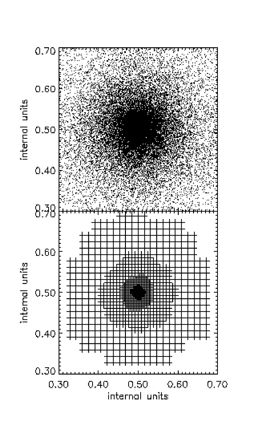
Figure 3: Refinement structure for Hernquist model sampled by $32^{3}$ particles and using $\rho_{\rm ref}=8$ particles per node.

5 Performance of the Poisson solver

The writers of $N$-body codes traditionally check the accuracy of their Poisson solver by using it to calculate the force between two point masses at various separations. In our view this test is misguided because a Poisson solver that is adapted to the solution of the collisionless Boltzmann equation should not return the force between point particles. At some level this fact is widely recognized in that a ‘softened’ interparticle force is aimed at, but isotropy of the interparticle force is still considered desirable. A Poisson solver for collisionless dynamics is concerned with finding the forces generated by smooth mass distributions. A single particle corresponds to a mass distribution that is unresolved on any smoothing scale, and thus one that falls outside its remit. Presented with this ill-posed problem, the best it can do is to assume that the density is non-zero in the cells around the particle, and zero elsewhere. Inevitably, this mass distribution reflects the geometry of the code’s cells, and it will not generate an isotropic gravitational field.

When testing a Poisson solver we should check its ability to recover the potential of density distributions of the type that it will encounter in the field. We have tested our code by comparing with analytic results the forces it generates for (a) a Hernquist model, and (b) a plane wave.

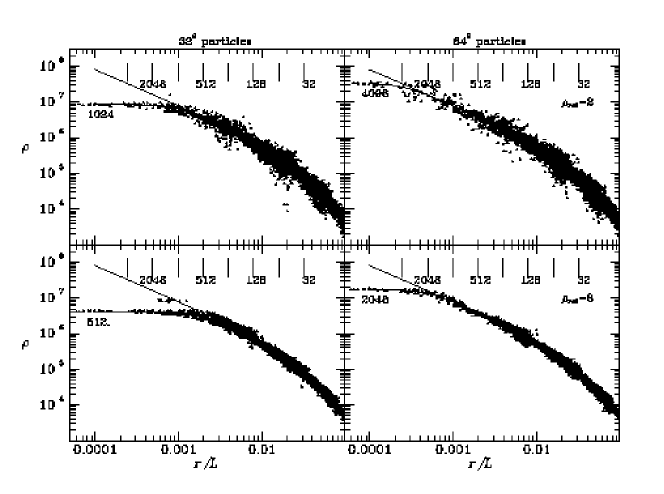
Figure 4: Recovery of the density profile of a Hernquist model from particle positions. For the left panels $32^{3}$ particles sampled a Hernquist profile, shown as the upper curve, with scale radius ${\textstyle{1\over 16}}$ of the box size and outer cutoff half the box size, $L$. For the right panels $64^{3}$ particles sampled the same profile. For all panels the domain grid had 32 nodes on a side. For the upper panels a node was refined if its density exceeded two particles per node, while for the lower panels the refinement threshold was eight particles per node. The tick marks along the top show the sizes of cells of grids with 4098, 2048, …, nodes on a side. The lower curves show the effect of doubly convolving the Hernquist profile with the TSC mass-assignment kernel. In the lower left panel, a small number of particles lie above the main mass near $r/L=0.001$. This phenomenon reflects the creation of a small refinement centred on the region of maximum density, which Poisson noise has displaced slightly from the centre of the probability distribution ($r=0$). In most realizations this feature is absent.

5.1 Hernquist model

We check the reliability of our refinement procedure and investigate the origin of errors in the force, by sampling a Hernquist model, in which the density varies with radius as

$$\rho(r)={Mr_{0}\over 2\pi}{1\over r(r_{0}+r)^{3}}.$$ (14)

The scale length $r_{0}$ of the Hernquist model was set equal to ${1\over 16}$ of the box size, and we calculated the potential with a domain grid $32$ nodes on a side. The model was truncated at a radius of $16$ grid nodes and a uniform background density was added to make the mean density within the box equal to a predetermined cosmic value; in practice about 3/7 of all particles were associated with the background. Our analytic calculations of the force do not include contributions coming from outside the box, where the periodic boundary conditions ensure that there are infinitely many other Hernquist models.

5.1.1 Refinement Hierarchy

Fig. 3 gives a visual impression of our refinement hierarchy at work by showing the distribution of particles according to a Hernquist model sampled with $32^{3}$ particles, and the threshold for refining nodes was set to $\rho_{\rm ref}=8$ particles per node. Refinements are shown down to the level of $512^{3}$ (virtual) nodes. One can clearly see how the grid structure adapts to the actual particle/density distribution. Successively more accurate solutions to Poisson’s equation are achieved within regions of higher density, where better force resolution is required to follow properly the particle dynamics.

Figure 5: The distribution of particles and nodes over grids in the realizations of a Hernquist sphere shown in Fig. 4. Full histograms: the numbers of particles in each grid. Hatched histograms: the numbers of nodes in each grid. The normalization $N_{\rm part}$ equals $32^{3}$ or $64^{3}$ rather than the actual number of particles in the simulation, which is slightly larger, as explained in the text.

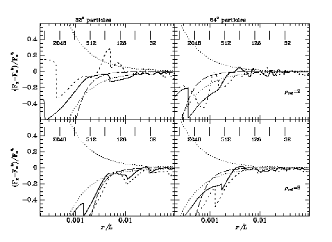
Figure 6: For the Hernquist model described in the text, the fractional difference between the values returned by MLAPM and obtained analytically for the $x$ component of the force. Distance from the centre of the sphere is plotted horizontally. The full curve is for values along the $x$-axis, while the short dashed curve is for values along the 111 direction relative to the axes. The upper panels are obtained when the critical density for refinement, $\rho_{\rm ref}$, corresponds to 2 particles per node, while the lower panels correspond to 8 particles per node.

5.1.2 Density estimates

It is important to know how accurately one can recover the density within a structure from the positions of particles that randomly sample it. The standard theorem of Monte-Carlo integration states that

$$\overline{\rho}({\bf{r}})\equiv\int{\rm d}^{3}{\bf{r}}^{\prime}\,W({\bf{r}}-{\bf{r}}^{\prime})\rho({\bf{r}}^{\prime})=\lim_{N\to\infty}{M\over N}\sum_{\alpha=1}^{N}W({\bf{r}}-{\bf{r}}_{\alpha}),$$ (15)

where the ${\bf{r}}_{\alpha}$ are positions distributed with probability density proportional to $\rho({\bf{r}})$. Applying this result to the case when $W({\bf{r}}-{\bf{r}}_{\alpha})$ is the fraction of the mass of a particle at ${\bf{r}}_{\alpha}$ that is assigned to a node at ${\bf{r}}$, we see that in the limit of infinitely many particles, the values of the density on the grid are not those of the input density $\rho$ but its convolution $\overline{\rho}$ with the mass-assignment kernel $W$. Moreover, if we use the same mass-assignment scheme to interpolate these values back to positions that are not on the grid, we recover

$$\overline{\overline{\rho}}({\bf{r}})\equiv\sum_{{\rm nodes}\ i}W({\bf{r}}-{\bf{r}}_{i})\overline{\rho}({\bf{r}}_{i}),$$ (16)

which is a discrete approximation to the convolution of $\overline{\rho}$ with the mass-assignment kernel. Hence, we expect density values recovered from the code to reflect not the input density but its double convolution with the mass-assignment kernel.

Fig. 4 shows that this expectation is borne out by showing four attempts to recover the density of the Hernquist sphere from the positions of either $32^{3}$ particles (left-hand panels) or $64^{3}$ particles (right-hand panels). In each case the recovered densities scatter around the result of doubly convolving the input density distribution with the TSC kernel for a grid with from 512 to 4096 nodes on a side. Increasing the particle number by a factor 8 causes finer grids to be generated, and thus enables the model’s $r^{-1}$ core to be traced further in. On the other hand, the variance in the estimated densities is not decreased by an increase in particle number. The upper panels show the result of refining nodes at a lower density threshold ($\rho_{\rm ref}=2$ particles per node) than the lower ones ($\rho_{\rm ref}=8$ particles per node). The reduction in variance and loss of resolution caused by an increase in the density threshold are evident. Also evident in the lower right panel is the increase in the variance as the edge of each grid is approached; at the outside of a grid the number of particles per node is smallest, and the variance correspondingly high.

Fig. 5 shows that lowering the critical density for refinement from eight to two particles per node does increase the maximum spatial resolution, but at considerable computational cost. Whereas with $\rho_{\rm ref}=8$ the ratio $n_{\rm node}/n_{\rm part}=0.75$ (for $64^{3}$ particles), this ratio rises to 3 when $\rho_{\rm ref}=2$. A node has a greater computational cost than a particle and it is less useful scientifically. Resources spent on lowering $\rho_{\rm ref}$ would be better spent increasing the number of particles.

In all four realizations the vast majority of nodes belong to the grids with less than 256 nodes on a side. Figs. 4 and 6 below show that on these scales little is gained by using a low value of $\rho_{\rm ref}$ – the gains from lowering $\rho_{\rm ref}$ are concentrated at small radii and derive from grids that contain small numbers of nodes and particles. In fact the numbers of nodes in the 4096³ grid in the top-right panels of Figs 4 and 6 are so small that they cannot be seen in Fig. 5. These findings suggest that significant gains in efficiency could be obtained by basing the refinement criterion on the truncation error in the forces rather than on the density. However, implementing this proposal is a job for the future.

5.1.3 Force estimates

Fig. 6 is similar to the Fig. 4 but for the estimated gravitational field ${\bf{F}}$ of the Hernquist model. Again left panels show results obtained with $32^{3}$ particles and right panels results for $64^{3}$ particles, and the upper and lower panels are for $\rho_{\rm crit}=2$ and 8 particles per node, respectively. In each panel the dotted curves show the loci $y(r)=\pm[\overline{N}(r)]^{-1/2}$, where $\overline{N}(r)$ is the expected number of particles interior to $r$. These curves show the minimum variance from Poisson noise: the true variance will be larger because density fluctuations are not constrained to be spherically symmetric. The full curve shows the difference between the analytic and numerical values of $F_{x}$ as a function of radius along the $x$ axis, while the short dashed curve shows the same quantity along the line $(1,1,1)$. These two curves agree with one another to within the anticipated Poisson errors, which shows that grid-generated anisotropy is not a problem. The long-dashed curves show the error expected because even in the limit of infinitely many particles the mass-assignment scheme recovers not the true density but its double convolution with the mass-assignment kernel. It is evident that the variance and the bias in the forces are fully accounted for by Poisson noise and smoothing by the mass-assignment kernel.

This conclusion is confirmed by a test in which the analytic value of the density was placed on every node before solving for the forces: on grid nodes the resulting forces agreed with the analytic ones to better than $0.2$ percent at all points, and to better than $0.05$ percent further from the centre than $2\Delta$ for the finest grid.

Figure 7: Bias and variance with two values of $\rho_{\rm ref}$. The dashed curves shows the relative error in the force of the Hernquist sphere that arises because the density is twice convolved with the mass-assignment kernel. The full curves show the rms variation in the force between different realizations of the system. All curves are for the case of $32^{3}$ particles except the second full curve in the lower panel, which is for $64^{3}$ particles. (It is on top at $r<0.001L$.)

The discussion above can be summarized by saying that the errors in the forces are dominated by uncertainty in the density. The latter is made up of a systematic bias due to any unresolved core, and variance due to Poisson noise. Increasing the particle number at fixed $\rho_{\rm ref}$ decreases the bias while holding the variance constant. Increasing the threshold density $\rho_{\rm ref}$ diminishes the variance and increases the bias. Fig. 7 quantifies this last statement by plotting the bias in the force from the left two panels of Fig. 6 as dashed curves, and the rms variation in the force between different realizations of the models as full curves. The latter decline outwards as the potential fluctuations caused by local density fluctuations, which are always of order $(\rho_{\rm ref})^{-1/2}$ times the local density, are increasingly swamped by the barely changing mean inward pull of the model. This dilution of the effects of density fluctuations is more marked in more massive systems, and less marked in less massive ones. Since all halos start out as small systems, we cannot rely on dilution of fluctuations to make our simulations credible. We have to recognize from Fig. 7 that the uncertainty in the forces can be reduced only by increasing $\rho_{\rm ref}$, and thus reducing the simulation’s spatial resolution. In particular, the introduction of a Particle–Particle step to harden the inter-particle forces at small separations would be analogous to lowering $\rho_{\rm ref}$ and therefore increasing the Poisson noise. We shall see in Section 5.2 below that our inter-particle force has a softening length of order $2\Delta$, or about four times the inter-particle separation when $\rho_{\rm ref}=8$. Simulations with both P³M and tree codes typically employ softening lengths that are substantially smaller than the initial inter-particle separation. Such small softening lengths are used because in these codes the softening length is fixed in either physical or comoving coordinates, so a small, and initially inappropriate value is required if high-density regions are to be adequately resolved once they have collapsed and virialized. With our method the softening length automatically adapts to some multiple of the local interparticle separation.

Fig. 7 suggests that the smallest permissible value of $\rho_{\rm ref}$ is 8 particles per node, which restricts fluctuations in forces near the centres of structure to the 20–30 percent level. The range of radii over which we have a reasonable representation of the underlying model, runs outwards roughly from the radius at which the bias falls below the variance. From Fig. 7 we see that with $32^{3}$ particles the range is $r>0.005L$, and in this range the forces are accurate to better than $10$ percent. With more particles the range would have a smaller lower limit, but the maximum uncertainty in the forces would increase towards $\sim 25$ percent in the limit of very large $N$.

As explained at the end of Section 4.4, the sum of all the forces on the particles cannot be expected to vanish since our softening is adaptive. Quantitatively, for $64^{3}$ particles and $\rho_{\rm ref}=2$ particles per node, we find

$$\left|\sum_{i}{\bf{F}}_{i}\right|=1.4\times 10^{-4}\sum_{i}|{\bf{F}}_{i}|.$$ (17)

When the same number of particles are distributed in a complex clustering pattern that evolved from realistic cosmological simulation, the coefficient in this equation was $4.7\times 10^{-4}$. In the absence of refinements, the coefficient was $2.7\times 10^{-7}$, and thus zero to the precision of a floating-point variable.

5.2 Zel’dovich waves

We now turn from virialized structures, to explore the performance of MLAPM before such structures form. Specifically, we compare the forces it generates with analytic results for plane waves.

Let ${\bf{r}}$ be Eulerian coordinates and ${\bf{q}}$ Lagrangian coordinates for an ensemble of particles that are uniformly distributed in ${\bf{q}}$-space. Then for $a(t)$ a suitable function of time that increases from zero to unity, the mapping

$${\bf{r}}={\bf{q}}+{a{\bf{k}}\over k^{2}}\cos({\bf{k}}.{\bf{q}})$$ (18)

with ${\bf{k}}$ a constant vector, generates a density field in ${\bf{r}}$-space that provides an exact solution for the development of a plane-wave cosmological perturbation in a flat universe (Zel’dovich 1970). The corresponding forces are readily obtained by differentiating ${\bf{r}}$ twice with respect to time.

Figure 8: Forces from a pure PM code of Zel’dovich waves described by equation (18) with $a=0.9$. In the top row ${\bf{k}}=(4\pi/L,0,0)$ and in the bottom row ${\bf{k}}=(18\pi/L,0,0)$. In every panel the wave is sampled with $32^{3}$ particles, and the grid has 32, 64 and 256 nodes on a side as one runs from left to right. Analytic forces are marked by squares and numerical ones by triangles.

Figure 9: The density (top) and forces (bottom) of a Zel’dovich wave with ${\bf{k}}=(18\pi/L,0,0)$ recovered by MLAPM from the positions of $32^{3}$ particles. The domain grid has 32 nodes on a side. As in Fig. 8, analytic values are marked by squares and numerical ones by triangles.

Fig. 8 explores the ability of a simple PM code to recover the forces generated by Zel’dovich waves with two values of $k$ and $a=0.9$. In every panel, the forces are recovered from the positions of $32^{3}$ particles. As one passes from left to right the number of nodes on a side of the grid rises from 32 to 256. With as many nodes as particles the forces are slightly in error for the longer wave and seriously in error for the shorter one. When there are eight times as many nodes as particles, the forces are reasonably accurate for both waves. With yet larger numbers of nodes unphysical force spikes either side of the plane on which the wave will break. One may readily demonstrate that these spikes arise because particles approach each other very closely as the wave breaks, and with a hard particle-particle interaction the overall force on a particle can be dominated by the contribution from a single neighbour. In the case of the shorter wave, the unphysical spikes make nonsense of the returned potential. This experiment nicely demonstrates the importance of tuning the softening of the potential to the resolution limit that is inherent in the number of particles.

Fig. 9 shows the density (top) and forces (bottom) that MLAPM generates with $32^{3}$ particles, a domain grid that has 32 nodes on a side and three values of the threshold density $\rho_{\rm ref}$. The most accurate forces are obtained with $\rho_{\rm ref}=1$ particle per node. Lower values again generate unphysical force spikes. Fig. 10 shows that an AP³M code also generates force spikes if the softening parameter is smaller than the inter-particle separation.

Figure 10: As Fig. 9 but showing forces recovered by Couchman’s AP³M code using a grid with as many ($32^{3}$) nodes as particles for three values of the force softening.

To produce the results shown in Fig. 9 for $\rho_{\rm ref}=1$ particle per node, MLAPM refines most nodes of the domain grid once and none twice. Consequently, there are $7.4$ nodes per particle, only slightly less than if we had started with a domain grid eight times larger and $\rho_{\rm ref}$ chosen to avoid refinement. We therefore have two strategies for obtaining adequate resolution in unvirialized regions. In one strategy, the domain grid has as many nodes as there are particles but we set $\rho_{\rm ref}$ on the domain grid to a small enough value that it is essentially all refined. Strictly we should ensure that the domain grid remains refined even in voids until the density has fallen to $\sim\overline{\rho}/8$, and this requires $\rho_{\rm ref}\simeq 0.25$ particles per node. In practice such small values of $\rho_{\rm ref}$ will be useful only at very late stages of a simulation, because the second strategy is more economical so long as the value of $\rho_{\rm ref}$ chosen under the first causes the whole domain grid to be refined. In the second strategy, one starts with a domain grid that has eight times as many nodes as particles, and sets $\rho_{\rm ref}=8$ on it because it provides adequate resolution until virialized structures form. With many PM and P³M codes, including the ART code, it is standard practice (but not mandatory) to use such a large domain grid. In certain circumstances this second strategy may be impossible on a given machine for a given number of particles. Then the first strategy can be adopted with $\rho_{\rm ref}$ set to the lowest value that is compatible with the available hardware. So long as $\rho_{\rm ref}$ is comparable to or smaller than unity, our experiments suggest that the correlation function and mass functions obtained differ insignificantly from those obtained with the second strategy (see Figs. 15 to 17 below).

Why is the optimal value of $\rho_{\rm ref}$ for Zel’dovich waves so much lower than that appropriate for virialized structures? Why are Zel’dovich waves best represented when 7/8 of the nodes are empty, and the remainder contain only one particle? There are two points to consider. (i) The TSC mass-assignment algorithm distributes the mass of a particle over 27 nodes, so a node may be empty and yet have non-zero density. (ii) A distribution of particles placed on a Zel’dovich distorted grid differs markedly from the particle distribution of a virialized body in that its underlying density field is uniquely defined by the particles (Appendix A). Hence, at early times the density field in a cosmological simulation is defined up to the scale of the inter-particle separation. Since the matter distribution is represented by particles, there is a great deal of artificial power on smaller scales, but this power is rather cleanly separated from the lower-frequency power that represents real cosmic fluctuations. As density gradients steepen gravitationally, this separation becomes less clean, and it breaks down completely with the formation of caustics and virialized structures. Consequently, in virialized regions the density field is dominated by Poisson noise at the scale of the inter-particle separation.

6 Integrating the equations of motion

We now turn from the Poisson solver to consideration of how particles are moved.

6.1 Time-stepping

The Lagrangian for motion in comoving coordinates is

$${\mathcal{L}}={\textstyle{1\over 2}}a^{2}\dot{x}^{2}-{\Phi\over a},$$ (19)

so the canonical momentum is

$$p=a^{2}\dot{x},$$ (20)

and the Hamiltonian is

$${\mathcal{H}}={p^{2}\over 2a^{2}}+{\Phi\over a}\ .$$ (21)

Hamilton’s equations are therefore

$$\begin{array}[]{lcc}\displaystyle{{\rm d}x\over{\rm d}t}&=&\displaystyle{p\over a^{2}}\\ \\ \displaystyle{{\rm d}p\over{\rm d}t}&=&\displaystyle-{\nabla\Phi\over a}\ .\end{array}$$ (22)

We integrate these equations with a minor variant of the usual symplectic scheme of second-order accuracy

$$x_{n+1/2} = x_{n}+p_{n}\int_{t}^{t+\Delta t/2}{{\rm d}t\over a^{2}}$$

$$p_{n+1} = p_{n}-\nabla\Phi(x_{n+1/2})\int_{t}^{t+\Delta t}{{\rm d}t\over a}$$ (23)

$$x_{n+1} = x_{n+1/2}+p_{n+1}\int_{t+\Delta t/2}^{t+\Delta t}{{\rm d}t\over a^{2}},$$

where the integrals can be evaluated analytically because they depend only on the cosmology. The implementation of multiple timesteps described below requires that positions and momenta be synchronized at the start and end of each timestep, so we do not form the standard leapfrog scheme by combining the drift steps that start and finish the above sequence of updates.

On finer grids forces tend to be larger, and the time it takes a particle to cross a cell is shorter. Hence shorter timesteps are appropriate for finer grids. Our time-stepping routine, STEP, is called recursively. It takes as arguments a grid, $G$, and a time interval, $\Delta$. STEP starts by asking whether any part of the grid $G$ should be refined. If the answer is ‘no’ it uses equations (6.1) to advance the particles on $G$ by $\Delta$ and then returns. If refinement is in order, a refined grid $G^{\prime}$ is created and STEP($\Delta/2,G^{\prime}$) called. That is, the particles on $G^{\prime}$ are advanced by $\Delta/2$ with the particles on $G$ still at the initial time. Once $G^{\prime}$ has been advanced in this way, STEP uses equations (6.1) to advance the particles still on $G$ by $\Delta$, and then calls STEP($\Delta/2,G^{\prime}$). STEP then erases $G^{\prime}$ and returns. This scheme is sketched by the following pseudo $C$-code:

Step(dt, CurrentGrid){
  NewGrid = Refine(CurrentGrid);
  if(NewGrid){
    Step(dt/2, NewGrid);}
  MoveParticles(dt, CurrentGrid);
  if(NewGrid){
    Step(dt/2, NewGrid);
    Destroy(NewGrid);}}

Fig. 11 summarizes this sequence of operations, which was proposed by Quinn et al. (1997). Whereas the coarse-grid timestep involves accelerations calculated with all particles at the half-time point, the two fine-grid steps involve accelerations calculated when the coarse-grid particles are first $\Delta/4$ behind the fine-grid ones, and then ahead of them by the same amount. The principle of the scheme is that errors arising from these lags cancel through second order in $\Delta$.

STEP is first called on the finest domain grid with a rather large value of $\Delta$. Through the recursive principle this call invokes calls on finer and finer grids with smaller and smaller vales of $\Delta$ until a grid is reached that requires no refinement, and it is advanced, so that the grid above can be advanced, and so on. Since refinements are destroyed after particles on them have been moved just twice, they always faithfully reflect the particle distribution.

The harmony of the above scheme is unfortunately marred by particles that leave the refinement from which they started before STEP has finished. Such departures cannot be ignored because a particle cannot continue to contribute to the density once it is outside the grid to which it is attached. Consider first particles that leave their refinement at any time up to the end of ‘1. fine-grid step’ in Fig. 11. We set the positions and velocities of such particles back to the values they had at $t_{n}$ and transfer them to the coarse grid as soon as they try to leave the refinement (which may be at $t_{n+1/4}$ or at $t_{n+1/2}$). Hence, a particle moves with a fine-grid time-step only if it both begins and finishes such a fine-grid step within the refinement. Particles that leave the refinement at $t_{n+3/4}$ during ‘3. fine-grid step’ in Fig. 11 are treated differently: such particles are immediately transferred to the coarse grid and added to the refinement’s list of ‘leavers’. The forces are then evaluated at $t_{n+3/4}$, and the velocities and positions of leavers are updated in parallel with the coordinates of particles that remained on the refinement. Since the refinement is destroyed at $t_{n+1}$, no significance attaches to a particle leaving the refinement as its position is updated to $t_{n+1}$.

No special action is taken when a particle enters the space occupied by a refinement during a call to STEP; the particle remains linked to a coarse-grid node that has been refined, and contributes to the density on both the coarse grid and its refinement with the spatial resolution characteristic of the coarse grid. (For a discussion of how particles attached to a coarse grid contribute to the density on a refinement, see Appendix B.)

The timesteps are sufficiently short that the movement of particles on grid $n$ cannot change the density on grids $n-2$ and higher. Consequently, drifting and kicking the particles on grid $n$ only requires mass assignment and relaxation of the potential to be performed on grids $n-1$ and $n$, so timesteps for the relatively small number of particles on the finest grids are computationally inexpensive.

Figure 11: The principle of the recursive time-stepping scheme in the case that part of the grid being operated on requires refinement. The fine-grid steps 1 and 3 are accomplished by calling the full stepping routine again and will typically involve further grid refinements. The coarse-grid step 2 involves updating particles not previously moved with the forces calculated with all particles advanced to the half-time point.

6.2 Internal Units

Let $H_{0}$ be the present Hubble constant, $B$ the present size of the computational box and $\overline{\rho}$ the mean matter density. The code uses the dimensionless variables

$$\begin{array}[]{lcl}x_{c}&=&x/B,\\ p_{c}&=&p/H_{0}B,\\ t_{c}&=&tH_{0},\\ \Phi_{c}&=&\displaystyle\Phi H_{0}^{2}B^{2},\\ \rho_{c}&=&\displaystyle\rho/\overline{\rho}.\end{array}$$ (24)

In terms of these variables, the equations to be solved are

$${{\rm d}x_{c}\over{\rm d}t_{c}} = {p_{c}\over a^{2}},$$

$${{\rm d}p_{c}\over{\rm d}t_{c}} = -{\nabla\Phi_{c}\over a},$$ (25)

$$\nabla_{c}\Phi_{c} = {3\Omega_{\rm M}\over 2}(\rho_{c}-1).$$

6.3 Dynamical evolution of Zel’dovich waves

In Section 5.2 we checked the accuracy of our Poisson solver. Here we check our time-stepping scheme by investigating its ability to reproduce the analytic solution for the breaking of a one-dimensional plane wave (Klypin & Shandarin 1983; Efstathiou et al. 1985). Since the initial conditions of a general cosmological simulation are a superposition of such waves, the ability to follow the evolution of a plane wave is a crucial test of the code.

We have used MLAPM with $\rho_{\rm ref}=1$ particle per node and Couchman’s (1991) AP³M code with $\epsilon=\Delta$ with $32^{3}$ particles on a $32^{3}$ domain grid to integrate the Zel’dovich wave from the initial conditions that are given by equation (18) and its counterpart for the momenta

$$p={{\dot{a}}^{3/2}{\bf{k}}\over k^{2}}\cos({\bf{k}}.{\bf{q}}).$$ (26)

Waves with three different values of $k$ were evolved with 200 timesteps on the domain grid from $a=0.1$ until $a=1$, when they break. We quantify the differences between the numerical and analytical solutions by evaluating the RMS deviations (Efstathiou et al. 1985)

$$\begin{array}[]{l}\Delta x_{\mbox{\tiny rms}}=\left[\sum_{i}(x_{i}-x_{i}^{\rm a})^{2}\ /\ \sum_{i}(x_{i}^{\rm a}-q_{i})^{2}\right]^{1/2}\\ \\ \Delta v_{\mbox{\tiny rms}}=\left[\sum_{i}(v_{i}-v_{i}^{\rm a})^{2}\ /\ \sum_{i}(v_{i}^{\rm a})^{2}\right]^{1/2}\ ,\end{array}$$ (27)

where the super-script $a$ denotes the analytical solution [eqs. (18) and 26)]. For each value of $k$ Table 1 shows errors from four calculations. The first and second rows show the overall errors from AP³M and MLAPM. These are broadly comparable. The MLAPM errors contain three contributions: (i) errors in the values of the forces at grid points; (ii) errors in the interpolation of these forces to the locations of particles; (iii) errors in updating of positions and momenta given the forces. The bottom row in Table 1 shows that this last source of error is insignificant by showing the errors one obtains when the force applied to each particle is the analytic value at its location. The penultimate row shows the much larger errors obtained when analytic forces are placed on the grid points: evidently interpolation is a significant source of error. Since the interpolation errors are of order a third of the overall errors shown in the second row, there is a suggestion that we are determining the density and then solving Poisson’s equation as accurately as is profitable given the coarseness of our grid.

Table 1: RMS errors in the positions ($\Delta x_{\mbox{\tiny rms}}$) and velocities ($\Delta v_{\mbox{\tiny rms}}$) of $32^{3}$ particles as defined by equation (27) for AP³M with $\epsilon=\Delta$ and MLAPM with a $32^{3}$ domain grid and $\rho_{\rm ref}=1$ particle per node

simulation	$kL/2\pi=1$		$kL/2\pi=2$		$kL/2\pi=9$
	$\Delta x$	$\Delta v$	$\Delta x$	$\Delta v$	$\Delta x$	$\Delta v$
AP3M	0.006	0.028	0.018	0.061	0.116	0.265
MLAPM	0.016	0.034	0.015	0.063	0.055	0.634
MLAPM(A1)	0.002	0.012	0.003	0.026	0.011	0.193
MLAPM(A2)	0.003	0.006	0.004	0.006	0.001	0.006

7 $\Lambda$CDM simulations

In this section we explore the performance of MLAPM when used to generate a realistic simulation.

Table 2: Parameters used for three comparing simulations performed with the ART, AP³M, and GADGET code.

ART	domain grid	$128^{3}$
	domain steps	500
	$\rho_{\rm ref}$	8/8
	refinement level reached	5
	number of GS sweeps on refinements	10
	CPU time	47 hr
AP3M	softening	$5h^{-1}\,{\rm kpc}$
	steps	4000
	particles per chaining-mesh cell	50
	refinements generated	89
	refinement level reached	4
	CPU time	69 hr
GADGET	softening	$5h^{-1}\,{\rm kpc}$
	velocity scale	$10{\rm kms}^{-1}$
	error tolerance angle	0.3
	tree accuracy	0.02
	tree update	0.05
	CPU time	58 hr

7.1 Simulation Parameters

We present data for simulations run with MLAPM, ART (Kravtsov et al. 1999), GADGET (Springel, Yoshida & White 2000) and the AP³M code (Couchman 1991). All six simulations contained $64^{3}$ particles distributed through a box $15h^{-1}\,{\rm Mpc}$ on a side. The simulations started from redshift $z=25$ with a $\Lambda$CDM spectrum of fluctuations. Table 2 lists the parameters employed in the ART, AP³M and GADGET simulations, while Table 3 gives the parameters of the three MLAPM runs. By their end-points, all MLAPM simulations had nodes associated with grids of $4096^{3}$ virtual nodes which agrees with the finest refinement level reached in the ART run (level 5).

The parameters given in the first row of Table 3 are chosen to mimic the behaviour of the ART code as closely as possible; ART is similar to MLAPM in many ways as both codes are purely grid based. They both use a regular domain grid covering the whole computational volume, and sequentially refine patches of high density with finer and finer refinement grids of arbitrary shape. The equations of motion are integrated using a multiple time stepping scheme that employs half the time step of the previous level on every given refinement. But there are subtle differences, too. The first, most obvious difference is the way the solution is obtained on the finest domain grid: ART uses an FFT solver whereas MLAPM utilizes Brandt’s multigrid scheme (Brandt 1977). Moreover, MLAPM uses the Triangular-Shape-Cloud (TSC) mass assignment scheme in contrast to the Cloud-In-Cell (CIC) scheme applied by ART. The equations of motion in the ART code are integrated using the expansion factor $a$ as integration variable, which was also applied to MLAPM’s ‘run $a$’ to make those two runs as similar as possible. Two other MLAPM runs ($t$1 and $t$2) use time $t$ for integrating the equations of motion (cf. Eq. 21 in Section 6) and perform 50 percent more Gauss-Seidel sweeps on each grid before checking for convergence. The latter results in a lower performance in terms of time, but should lead to more accurate solutions of Poisson’s equation. We will investigate these propositions in more detail below.

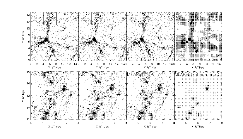
Figure 12: Slice through three $\Lambda$CDM simulations run from identical initial conditions using (from left to right) GADGET, ART, and MLAPM (run $a$). The extreme right-hand panels show the final grid hierarchy of the MLAPM simulation. The bottom panels show enlargements of the small region marked in the upper panels.

Table 3: Parameters of MLAPM simulations. The value for the number of domain grid cells is given in the second column and the number of integration steps also applies for the domain grid. The first number in the $\rho_{\rm ref}$ column is the refinement density on the domain grid, while the second number applies to all finer grids. The same convention applies in the column headed ‘GS sweeps’. The simulation plotted in Fig. 12 corresponds to run $a$ which parameters were chosen as close as possible to the ones in the ART run.

run	grid	$\rho_{\rm ref}$	steps	GS sweeps	CPU time
$a$	$128^{3}$	8/8	500	10/10	$42\,$hr
$t$1	$128^{3}$	8/8	500	15/15	$69\,$hr
$t$2	$64^{3}$	1/8	250	15/15	$48\,$hr

7.2 Comparisons

Fig. 12 shows slices through the GADGET and ART simulations, and the MLAPM simulation that corresponds to the first row of Table 3 (run $a$). The lower panels show enlargements of a small region of the upper panels. The rightmost panels show the final grid structure of the MLAPM simulation. The three particle distributions are clearly very similar, but not identical. In comparisons between simulations run with AP³M and ART, Knebe et al. (2000) detected similar differences, and showed that understanding the physical significance of these differences is not straightforward. In particular, simulations run with different codes tend to be at slightly different phases at a given time. Such phase differences are probably not physically significant, but can lead to material differences in the appearance of slices such as those shown in Fig. 12. For example, in one panel a small cluster may be evident while in another it is invisible because its centre lies just above or below the slice shown.

It is now interesting to compare MLAPM (run $a$) with the ART run as both are set up as similarly as possible. In Fig. 13 we therefore plot for both codes the refinement level reached against the expansion factor $a$. From $a\sim 0.55$ onwards no finer refinements are generated and hence there is no need to extend the plotted data to $a=1$. We can clearly see that both codes start using the same refinements at about the same time, with ART creating its levels slightly earlier. Otherwise the curves agree fairly well, demonstrating how similarly MLAPM and ART are dealing with refinements. The ‘noisy behaviour’ can be ascribed to the small size of refinements when they are first created; all adaptive grids are placed around initially small high density regions, which might fluctuate around the density threshold for a couple of steps until stabilized. To compensate for this effect MLAPM refines at the beginning of each domain grid step down to the actually needed refinement level but does not allow finer grids to be called into existence during the course of that domain step. This might explain why MLAPM’s refinements appear to be invoked slightly later than ART’s (Fig. 13).

Figure 13: Refinement levels invoked by MLAPM (run $a$) and ART (dashed curve) as a function of the expansion factor.

Figure 14: CPU time used as a function of the expansion factor reached for the simulations shown in Fig. 12 and three other MLAPM simulations. The curve for the MLAPM simulation plotted in Fig. 12 finishes second from the bottom.

Fig. 14 shows, again as a function of expansion parameter $a$, the CPU time required by all six simulations. Since the speed with which a given code runs depends sensitively on the values chosen for its various (technical) parameters, exact comparisons are difficult to make. Experiments with slightly modified parameters for ART, GADGET, and AP³M showed that the total times needed to run a simulation can vary by up to 50% without perceptible change in the statistical analysis as given below. The only difference between MLAPM’s run $a$ and run $t$1, besides the integration variable, is the number of GS sweeps performed on each grid before checking for convergence. As most of the time is spent on solving Poisson’s equation, we get an increase of more than 60% in time when using 50% more sweeps; we also observe slightly bigger refinements in run $t$1 which accounts for the remaining 10% decrease in performance.

It is also worth noticing that AP³M and ART both perform similarly at early times, when the forces are (mainly) based on an FFT solver. Only when particles start to cluster and the PP part becomes more and more important in the AP³M run does ART start to show its advantage by using arbitrarily shaped refinements in high density regions to increase the force resolution. However, MLAPM overtakes ART at times, when the use of refinements is dominating the time budget. This behaviour suggests that our (de-)refinement procedure is more time efficient and indicates that the difference in performance at early times between ART and MLAPM can be ascribed to our adoption of Brandt’s multigrid plan even on the domain grid. But again, checking the relative timings of an FFT solver and the multi-level algorithm is a job for the future.

Figure 15: Power spectra at redshift $z=0$ for all six simulations. The lower solid line is actually a superposition of broken lines.

In Fig. 15 we show the dark matter power spectra of all six simulations at a redshift $z=0$. There are no obvious differences and they all agree very well with each other.

However, when investigating the cumulative mass function $n(>M)$ for particle groups (Fig. 16) identified using a standard friends-of-friends group finder with linking length 0.17 (which corresponds to an overdensity of about 330), there are subtle deviations between the runs. At the high mass end they all coincide, but at the low mass end of the distribution function we observe more small objects in AP³M and (to a smaller extent) GADGET than in any of the other runs. This agrees with findings by Knebe et al. (2000), where it was shown that AP³M tends to form more low-mass objects in underdense regions (cf. Fig. 3 in that paper).

Figure 16: Mass functions at redshift $z=0$ for all six simulations. Halos were identified using a standard friends-of-friends algorithm.

Figure 17: Halo-Halo correlation functions at redshift $z=0$ for all six simulations. Halos were identified using a standard friends-of-friends algorithm.

Finally we show the halo-halo correlation function for the objects presented in Fig. 16 – the agreement between the codes is good.

These comparisons convince us that all four codes produce comparable results in comparable times, except that there are small differences in the mass functions produced by grid-based methods (MLAPM and ART) and PP-based ones (AP³M and GADGET). We also find that there are only modest changes in the scientific results when fiddling with the technical parameters, i.e. the number of GS sweeps.

7.3 MLAPM performance

This section deals with the dependence of MLAPM’s performance on the values taken by technical parameters and the way the grids are used.

Fig. 18 shows as a function of expansion factor achieved the numbers of nodes at each refinement level for two simulations: those listed in the second and third rows of Table 3 (runs $t$1 and $t$2). The growth in the grids with $256^{3}$ or more virtual nodes is identical in the two simulations and the last two levels ($2048^{3}$ and $4096^{3}$) are not shown for clarity. When the domain grid has $64^{3}$ nodes, the number of nodes in the $128^{3}$ grid falls by a factor 2.5 during the simulation, as particles drain out of voids and more and more domain-grid nodes fail to achieve the threshold for refinement, namely $\rho_{\rm ref}=1.0$ particles per node.

Figure 18: Numbers of nodes at each level of refinement as a function of expansion factor. Grids as fine as $4096^{3}$ virtual nodes are created, but data for the finest two grids are not plotted.

Comparison of the timings listed in the lower two rows of Table 3 (run $t$1 and $t$2) shows that MLAPM is slowed when the number of domain grid cells is changed from $64^{3}$ to $128^{3}$. This is explained in Table 4, where we show the average time spent on a given grid over the course of the whole simulation. Note, that in run $t$2 we are also doing 500 steps on the $128^{3}$ grid and our refinement criterion was chosen to refine (nearly) the whole domain grid at early times. As this run requires both less CPU time and less memory, it provides better value for money.

Table 4: Average CPU time in seconds per step over the course of a simulation with $64^{3}$ particles on a $64^{3}$ domain grid (run $t$2) and $128^{3}$ domain grid (run $t$1), respectively.

Grid:	64	128	256	512	1024
MLAPM $t$1:	—	261	18	5	2
MLAPM $t$2:	35	127	21	5	2

It is interesting to see how the CPU time required per step varies between grids. Again, Table 4 lists the average CPU time per step used to solve for the forces and move the particles on the first through fourth refinements in the course of the simulation whose end-point is plotted in the rightmost four panels of Fig. 12. It is always the $128^{3}$ grid which dominates the time budget, but even when we add up the time spent on the $64^{3}$ and the $128^{3}$ grid for run $t$2 we are still faster than using a regular $128^{3}$ grid all the time, because at later times there are far fewer nodes to sweep over (cf. Fig. 18). Thus the enhanced resolution that an adaptive grid provides in high density regions comes at an insignificant cost in both memory and CPU time.

7.4 Layzer–Irvine equation

A useful check on the accuracy of a cosmological simulation is provided by the Layzer–Irvine equation. To derive an appropriate form of this, we assume that the single-particle potential $\Phi$ that appears in the Hamiltonian (21) could be obtained by a sum over pairs of some time-independent smoothing kernel $S$. With this assumption the total potential energy of the system is

$${\displaystyle{U\over a}} = {\displaystyle{1\over 2a}\sum_{\alpha=1}^{N}\Phi({\bf{x}}_{\alpha})}$$ (28)

$$= {\displaystyle-{1\over 2a}\sum_{\alpha\neq\beta}S(|{\bf{x}}_{\alpha}-{\bf{x}}_{\beta}|),}$$

where the sum is over all particles and the coordinates are comoving ones. It is straightforward to check that our equations of motion (22) can be obtained from the $N$-body Hamiltonian

$$H={K\over a^{2}}+{U\over a},$$ (29)

where

$$K\equiv{\textstyle{1\over 2}}\sum_{\alpha=1}^{N}p_{\alpha}^{2}.$$ (30)

We have

$${{\rm d}H\over{\rm d}t} = {\partial H\over\partial t}$$ (31)

$$= -{\dot{a}\over a}\left({2K\over a^{2}}+{U\over a}\right).$$

Consequently

$$\left[H\right]_{t_{1}}^{t_{2}}=-\int_{t_{1}}^{t_{2}}{{\rm d}a\over a}\left({2K\over a^{2}}+{U\over a}\right).$$ (32)

This equation, which is valid no matter how $a$ depends on time, states that the Hamiltonian would be constant if the system were fully virialized. For some reason it is conventional not to monitor the satisfaction of this equation, but of an alternative conservation equation that follows from equation (31), namely

$${{\rm d}aH\over{\rm d}t} = \dot{a}H+a\dot{H}$$ (33)

$$= -\dot{a}{K\over a^{2}}\ .$$

Consequently

$$C\equiv[aH]_{t_{1}}^{t_{2}}+\int_{a_{1}}^{a_{2}}{\rm d}a\,{K\over a^{2}}$$ (34)

should be constant.

Figure 19: Variation with $a$ of the Layzer-Irvine invariant $C$ that is defined by equation (34).

Fig. 19 plots $C/|U|$ as a function of $a$ for all three MLAPM simulations. By taking smaller time-steps one can show that truncation error in the integration of the equations of motion (22) makes a negligible contribution to the variation of $C$. Errors in interpolating the forces from the grid to the locations of particles (see Section 5.1.3) cause $C$ to vary by causing the force on a particle to differ slightly from the local potential gradient. Another important contributor to the variability of $C$ is the fact that $\Phi$ cannot be obtained from a time-independent smoothing kernel $S(|{\bf{x}}|)$, as we assumed in deriving equation (34). Indeed, no such kernel would give our potential precisely, because our softening length $\epsilon$ diminishes from voids to the cores of clusters. Moreover, the mean value of $\epsilon$ diminishes over time as clustering develops and finer and finer grids are created. Since the Layzer–Irvine equation is based on the assumption of a spatially and temporally invariant softening kernel, it follows that variability of $\epsilon$, for which Section 5 presents a powerful case, will lead to significant violations of the Layzer–Irvine equation. This is also reflected in the curve for run $t$2 as in this case we started out with a $64^{3}$ domain grid and used a grid with $128^{3}$ virtual nodes that varied significantly in extent (cf. Fig. 18). However, the variation in $C/|U|$ is less than 2 to 3 percent except for a steep rise in $C$ during the very first steps, which is probably due to sharp changes in the resolution provided by the $128^{3}$ grid. As the calculation settles down there follows a more moderate decrease in $C/|U|$, which finishes at about 2 percent.

8 Discussion and Conclusions

In the coming years work with cosmological simulations will increasingly focus on the formation of galaxies of various types. Such simulations demand the highest attainable spatial and mass resolution and will stretch available computer power to its limits. The efficiency of the available computer codes, both in respect of CPU time and memory usage, will be of paramount importance. $N$-body codes can be divided into those that find the gravitational potential by summation over a Green’s function, and those that solve Poisson’s equation on a grid. To be efficient, the grid employed in the latter type of code has to be capable of adapting itself dynamically to the evolving mass distribution, and this requirement leaves one little option but to solve Poisson’s equation by Brandt’s multigrid technique.

The code presented here, MLAPM, is one of two cosmological codes that deploys such a grid, the other being the ART code (Kravtsov et al. 1997, 1999). Both codes subdivide cells in which the density exceeds a threshold, and move particles with timesteps that decrease by a factor 2 with each additional level of refinement of the region within which they lie. With these codes gravity is automatically softened adaptively, so that the softening length is near its optimum value in both high and low-density regions. With AP³M and most tree codes, by contrast, a single softening length is employed at all times and places, with the result that it is generally much smaller than it should be in low-density regions.

Although MLAPM and ART are conceptually very similar, they do differ in a number of important respects. In particular,

• MLAPM uses a simple recursive and fully symplectic integration scheme;

• since MLAPM is written in $C$ rather than FORTRAN, it can make extensive use of dynamic memory allocation;

• MLAPM uses Brandt’s multi-grid approach for solving Poisson’s equation even on the domain grid, whereas the ART code uses an FFT solver.

MLAPM has a single free parameter, the threshold density for node refinement, $\rho_{\rm ref}$. Smaller values of $\rho_{\rm ref}$ yield finer grids and harder forces. The memory used by grids is proportional to $\rho_{\rm ref}^{-1}$ and exceeds the memory used by particles for $\rho_{\rm ref}\mathrel{\hbox{\hbox to0.0pt{\hbox{\lower 4.0pt\hbox{$\sim$}}\hss}\hbox{$<$}}}8$ particles per node.

Tests of the ability of the code to recover the gravitational fields of virialized structures and strongly non-linear plane waves show that radically different values of $\rho_{\rm ref}$ are required in the two cases. With $\rho_{\rm ref}<8$ particles per node, forces near the centre of a typical virialized structure fluctuate from realization to realization by more than 25 percent. Hence, 8 particles per node seems a minimum value for $\rho_{\rm ref}$ when representing virialized halos.

By contrast, to recover a reasonable approximation to the field of a wave whose frequency exceeds half the Nyquist frequency of the domain grid with as many particles as the grid has nodes, we require $\rho_{\rm ref}\mathrel{\hbox{\hbox to0.0pt{\hbox{\lower 4.0pt\hbox{$\sim$}}\hss}\hbox{$<$}}}1$ particle per node, which ensures that the domain grid is refined through most of the simulation. Such a small value works well prior to virialization although it would yield a completely noise-dominated gravitational field after it, because the usual procedure for setting up the initial conditions of cosmological simulations enables the underlying density to be recovered from the particle positions, free of Poisson noise.

In view of the different refinement criteria required before and after virialization, one of two strategies should be adopted. In the first one uses a domain grid with as many nodes as there are particles, and on it sets $\rho_{\rm ref}$ to a value less than unity. This ensures that the domain grid is refined everywhere until voids develop in which the particle density is low enough for adequate resolution to be provided by the domain grid alone. In the second strategy, the domain grid has eight times as many nodes as there are particles, and one sets $\rho_{\rm ref}=8$ particles per node on every grid. The second strategy is safer unless clustering is so highly developed that the density is less than an eighth of the mean density in a significant volume. However, our experiments show that using a coarse domain grid with $\rho_{\rm ref}=1$ yields statistically indistinguishable results at lower cost than the conservative strategy.

Before a code for cosmological simulations can now be considered complete, it should include instructions written in MPI that will enable it to run on a distributed-memory multi-processor computer. To our knowledge only one such code is currently publicly available for cosmological $N$-body simulations, the tree code GADGET (Springel, et al. 2000). Producing an MPI version of MLAPM is a high priority. Multigrid codes are in principle well suited to parallelization because each subgrid of the domain grid can be advanced substantially independently of the others. Moreover, the data structures (nodes and quads) associated with physically connected nodes are already allocated in a way that makes them likely to be stored in adjacent blocks of memory, and the existing linking of particles to nodes means that it would be simple to ensure that data for physically connected particles were always stored together. The only significant problem we anticipate encountering in the parallelization arises from the recursive nature of the calls to step. Such recursive calls are known to be a barrier to parallelization. Fortunately, by making a few copies of STEP, called STEP0, STEP1, …, or whatever, it is trivial (if inelegant) to make the algorithm non-recursive, at least for the first few calls. Loops over $z$QUADS within one of these non-recursive copies of STEP could then be parallelized.

Appendix A: Density from mass on a Zel’dovich-distorted grid

We show that a distribution of particles placed on a Zel’dovich distorted grid uniquely defines the underlying density field. Consider the generalization of equation (18) to many waves, one for each site of a lattice in ${\bf{k}}$-space. We have that the $N$ particle displacements ${\bf{e}}_{\alpha}={\bf{r}}_{\alpha}-{\bf{q}}_{\alpha}$ are related to the amplitudes $A_{\bf{k}}$ of the generating waves by the finite sum

$${\bf{e}}_{\alpha}=\sum_{|{\bf{k}}|<K}{\bf{A}}_{\bf{k}}\cos({\bf{k}}.{\bf{q}}_{\alpha}).$$ (35)

If the particles are on the grid in ${\bf{q}}$-space that is the reciprocal of the ${\bf{k}}$-space grid, then this equation states that the ${\bf{e}}_{k}$ are related to the ${\bf{A}}_{k}$ by a DFT. Hence we can recover the latter from the particle positions and then reconstruct the entire density field from the Jacobian

$$\rho=\overline{\rho}\left[{\partial({\bf{r}})\over\partial({\bf{q}})}\right]^{-1}.$$ (36)

We have investigated the possibility of obtaining the density in regions that have yet to virialize from equation (36). We find that numerical differentiation of ${\bf{r}}$ with respect to ${\bf{q}}$ does yield more accurate values of the density than the TSC mass-assignment scheme, especially in voids. However, most of this advantage is lost in propagating the density from the locations of particles to nodes.

Appendix B: Particle transfer to fine grids

We describe intricacies that arise when particles transfer from coarser to finer grids. Fig. 20 shows five particles at or near the boundary of a refinement (which always includes fine nodes that are cospatial with coarse nodes). Assigning the masses of a particle such as P1 is straightforward because its mass only contributes to the density on the coarse grid. Similarly, the mass of P5 only contributes to the density on the fine grid. The masses of the other three particles contribute to the density on both grids, and considerable care has to be exercised in its assignment. The main problem is to determine the contributions to the fine grid of particles like P2 and P3 that remain on the coarse grid.

We start by transferring particles P4 and P5 to the fine grid. Next we use the coarse grid’s TSC kernel to subtract from coarse-grid nodes the mass of these particles, and the fine grid’s kernel to add the same mass to fine-grid nodes. At this stage mass is assigned to boundary nodes such as N1. When this has been done the density on a coarse-grid node such as N2 that lies in the interior of the refinement will be zero, while a coarse-grid node such as N3 that lies near the refinement’s edge will have non-zero density. In fact, the density on N3 will come from particles such as P2 and P3. We use the fine grid’s TSC kernel to distribute this mass among the neighbouring fine-grid nodes, but for the present we hold it in temporary variables, separate from the masses associated with P4 and P5. Now we use the restriction operator to add the fine-grid density to all coarse-grid nodes that are cospatial with a fine-grid node. This operation completes the determination of the coarse-grid density. Finally we complete the determination of the fine-grid density by adding to each fine-grid node the mass held in its temporary variable.

Figure 20: Particles and nodes at the edge of a refinement.

References

- [aarseth] Aarseth S.J., Turner E.L., Gott J.R., 1979, ApJ 228, 664
- [appel] Appel A.W., 1985, SIAM J.Sci.Stat.Comput. 6, 85
- [Barnes Hut] Barnes J., Hut P., 1986, Nature 324, 446
- [Brandt 1977] Brandt A., Math. of Comp. 31, 333 (1977)
- [Couchman 1991] Couchman H.M.P., 1991, ApJ Lett. 368, 23
- [dehnen] Dehnen W., 2000, ApJ Lett. 536, 39
- [dehnen] Dehnen W., MNRAS in press (astro-ph/0011568)
- [Efstathiou et al. 1985] Efstathiou G., Davis M., Frenck C.S., White S.D.M.,1985, ApJ Suppl. 57, 241
- [Frenk et al. 1999] Frenk, C., et al., 1999, , ApJ 525, 554
- [gingold] Gingold R.A., Monaghan J.J., 1977, MNRAS 181, 375
- [gnedin] Gnedin N.Y., 1995, ApJ Suppl. 97, 231
- [haggerty] Haggerty M.J., Janin G., Å364151974
- [Hockney & Eastwood 1988] Hockney R.W., Eastwood J.W., Computer Simulations Using Particles, Bristol: Adam Hilger (1988)
- [hohl] Hohl F., 1978, Astron. J. 83, 768
- [Klypin & Shandarin 1993] Klypin A.A. & Shandarin S.F., 1983, MNRAS 204, 891
- [Knebe et al. ] Knebe A., Kravtsov A.V., Gottlöber S., Klypin A.A., 2000, MNRAS 317, 630
- [Kravtsov et. al. 1997] Kravtsov A.V., Klypin A.A., Khokhlov A.M., 1997, ApJ 111, 73
- [Kravtsov 1999] Kravtsov A.V., 1999, PhD thesis, New Mexico State University, Las Cruces
- [leeuwin] Leeuwin F., Combes F., Binney J., 1993, MNRAS 262, 1013
- [lucy] Lucy L.B., 1977, Astron. J. 82, 1013
- [norman] Norman M.L., Bryan G.L., in Numerical Astrophysics, eds. S.Miyama, K.Tomisaka,T.Hanawa (Boston:Kluwer), 1998
- [Peebles] Peebles P.J.E., 1970, Astron. J. 75, 13
- [pen] Pen U.-L., 1998, ApJ Suppl. 115, 19
- [press] Press W.H., Schechter P., 1974, ApJ 187, 425
- [press] Press W.H., Teukolsky S.A., Vetterling W.T., Flannery B.P., Numerical Recipes, Cambridge Univ. Press, 1992
- [Quinn et. al. 1997] Quinn T., Katz N., Stadel J., Lake G., ApJ submitted, astro-ph/9710043
- [Spergel & Steinhardt] Spergel D.N., Steinhardt P.J., 2000, Phys. Rev. Lett. 84, 376
- [Springel et. al. 2000] Springel V., Yoshida N., White S.D.M., astro-ph/0003162
- [white] White S.D.M., 1976, MNRAS 177, 717
- [zeldovich] Zeldovich Y.B., 1970, A&A 5, 84