Determining cosmic microwave background structure from its peak distribution.

Abstract

We present a new method for time-efficient and accurate extraction of the power spectrum from future cosmic microwave background (CMB) maps based on properties of peaks and troughs of the Gaussian CMB sky. We construct a statistic describing their angular clustering - analogously to galaxies, the 2-point angular correlation function, $\xi_{\nu}(\theta)$. We show that for increasing peak threshold, $\nu$, the $\xi_{\nu}(\theta)$ is strongly amplified and becomes measurable for $\nu\geq$1 on angular scales $\leq 10^{\circ}$. Its amplitude at every scale depends uniquely on the CMB temperature correlation function, $C(\theta)$, and thus the measured $\xi_{\nu}$ can be uniquely inverted to obtain $C(\theta)$ and its Legendre transform, the power spectrum of the CMB field. Because in this method the CMB power spectrum is deduced from high peaks/troughs of the CMB field, the procedure takes only $[f(\nu)]^{2}N^{2}$ operations where $f(\nu)$ is the fraction of pixels with $|\delta T|\geq\nu$ standard deviations in the map of $N$ pixels and is e.g. 0.045 and 0.01 for $\nu$=2 and 2.5 respectively. We develop theoretical formalism for the method and show with detailed simulations, using MAP mission parameters, that this method allows to determine very accurately the CMB power spectrum from the upcoming CMB maps in only $\sim(10^{-4}-10^{-3})\times N^{2}$ operations.

Subject headings: cosmology - cosmic microwave background - methods: numerical

1. Introduction.

By probing the structure of the last scattering surface, the current and upcoming balloon and space borne missions promise to revolutionize our understanding of the early Universe physics. This requires probing the angular spectrum of the cosmic microwave background (CMB) with high precision on sub-degree scales, or angular wave-numbers $l>200$. For cold-dark-matter (CDM) models based on inflationary model for the early Universe and adiabatic density perturbations, the structure of the CMB should show the signature of acoustic oscillations leading to multiple (Doppler) peaks. The relative spacing of the Doppler peaks should then reflect the overall geometry of the Universe, whereas the amplitude of the second (and higher) peaks depends sensitively on other cosmological parameters, such as the baryon density, re-ionization epoch, etc. The recent balloon-borne measurements (de Bernardis et al., 2000, Mauskopf et al 2000, Hanany et al., 2000) strongly imply a flat cosmological model because the first Doppler peak occurs at $l\simeq 200$ (Kamionkowski, Spergel & Sugiyama 1994, Melchiori et al 2000, Jaffe et al 2001).

A major challenge to understanding these and future measurements is to find an efficient algorithm that can reduce the enormous datasets with $N\!\simeq\!10^{5}$ pixels in balloon experiments to $\simeq\!3\times\!10^{6}$ for MAP band with the 0.2^∘ beam (at 90 GHz) to $\simeq\!10^{8}$ for the Planck HFI data. Traditional methods require inverting the covariance matrix and need $\sim\!N^{3}$ operations making them impossible for the current generation of computers. Thus alternatives have been developed for estimating the CMB multipoles in O($N^{2}$) operations from Gaussian sky (Tegmark 1997; Oh, Spergel & Hinshaw 1999) and general CMB sky (Szapudi et al 2000) as well as study statistics of the various methods (Bond et al. 2000; Wandelt et al 2001).

In this letter we suggest a novel, accurate and time-efficient method for computing the angular power spectrum of the CMB temperature field from datasets with large $N$ using the properties of the peaks (and troughs) of the CMB field. The peaks are much fewer in number than $N$, but they will be strongly clustered. In Sec. 2 we construct a statistic describing their angular clustering - the 2-point angular correlation function $\xi$ in analogy to the galaxy correlation function (Peebles 1980), i.e. the excess probability of finding two peaks at a given separation angle. We show that this statistic is strongly amplified over the scales of interest ($<$10^∘) and should be measurable. The value of $\xi$ for a given peak threshold $|\delta T|\!\geq\!\nu\sigma$ would be uniquely related to the correlation function of the temperature field $C\!=\!\langle\delta T(\vec{x})\delta T(\vec{x}\!+\!\vec{\theta})\rangle$. The measurement of $\xi$ can then be uniquely inverted to obtain the underlying $C$ and its Fourier transform, the power spectrum $C_{l}$. This can be achieved in just $[f(\nu)]^{2}N^{2}$ operations, where $f(\nu)$ is the fraction of pixels with $|\delta T|\!\geq\!\nu\sigma$ and is e.g. 4.5–1% for $\nu$=2-2.5. Sec. 3 shows concrete numerical simulations for the MAP 90GHz channel in order to estimate cosmic variance, sampling uncertainties, instrumental noise etc. We show that with this method the CMB power spectrum is recovered to accuracy comparable to or better than by other existing methods but in a significantly smaller number of operations. On an UltraSparc II 450 MHz processor the entire sky map with 0.2^∘ angular resolution can be analyzed and $C_{l}$’s recovered in only 15 mins and 2.25 hours CPU time for $\nu=$2.5 and 2.1 respectively.

2. Method

For Gaussian ensemble of $N$ data points (e.g. pixels) describing the CMB data $\delta\equiv T-\langle T\rangle$ one expects to find a fraction $f(\nu)=$erfc($\nu/\sqrt{2})$ with $|\delta|\geq\nu\sigma$, where $\sigma^{2}=\langle\delta^{2}\rangle$ is the variance of the field and erfc is the complementary error function. E.g. $f(\nu)$=$(4.5,1,0.1)\!\times\!10^{-2}$ for $\nu$=(2,2.5,3) respectively. The joint probability density of finding two pixels within $d\delta_{1,2}$ of $\delta_{1,2}$ and separated by the angular distance $\theta$ is given by the bivariate Gaussian (the vector $\delta$ has components [$\delta_{1},\delta_{2}$]):

$$p(\delta_{1},\delta_{2})=\frac{1}{2\pi\sqrt{||\mbox{\boldmath$C$}||}}\exp(-\frac{1}{2}\mbox{\boldmath$\delta$}\cdot\mbox{\boldmath$C$}^{-1}\cdot\mbox{\boldmath$\delta$})=\frac{1}{(2\pi)^{2}}\int_{-\infty}^{\infty}\int_{-\infty}^{\infty}\exp(-i\mbox{\boldmath$q$}\cdot\mbox{\boldmath$\delta$})\exp(-\frac{1}{2}\mbox{\boldmath$q$}\cdot\mbox{\boldmath$C$}\cdot\mbox{\boldmath$q$})d^{2}\mbox{\boldmath$q$}$$ (1)

where $C$ is the covariance matrix of the temperature field. We model the covariance matrix in (1) as $C(\theta)=C_{0}\delta_{ij}+C(\theta_{ij})(1-\delta_{ij})$, where $\delta_{ij}$ is the Kronecker delta and $C_{0}\equiv C(0)+\sigma_{n}^{2}$; $\sigma_{n}$ is the noise contribution. We assume that the noise is diagonal, the entire CMB sky is Gaussian and the cosmological signal whose power spectrum we seek is contained in $C(\theta)=\sum(2l+1)C_{l}P_{l}(\cos\theta)/4\pi$. The total dispersion of the temperature field is then $\sigma=\sqrt{C(0)+\sigma_{n}^{2}}$

The peaks of a Gaussian field should be strongly clustered (Rice 1954, Kaiser 1984, Jensen & Szalay 1986, Kashlinsky 1987). The angular clustering of such regions can be described by the 2-point correlation function, i.e. the excess probability of finding two events at the given separation. The probability of simultaneously finding two temperature excursions with $|\delta T|\!\geq\!\nu\sigma$ in small solid angles $dw_{1,2}$ is $dP_{12}\!\propto\!(1+\xi)dw_{1}dw_{2}$. The correlation function of such regions is:

$$\xi_{\nu}(\theta)=\frac{2\int_{\nu\sigma}^{\infty}\int_{\nu\sigma}^{\infty}[p(\delta_{1},\delta_{2})+p(-\delta_{1},\delta_{2})]d\delta_{1}d\delta_{2}}{[2\int_{\nu\sigma}^{\infty}p(\delta)d\delta]^{2}}-1$$ (2)

The numerator follows from considering contributions from correlations between $\delta_{1},\delta_{2}$ in regions of 1) $\delta_{1}\!\geq\!\nu\sqrt{C_{0}}$, $\delta_{2}\!\geq\!\nu\sqrt{C_{0}}$; 2) $\delta_{1}\!\leq\!-\nu\sqrt{C_{0}}$, $\delta_{2}\!\leq\!-\nu\sqrt{C_{0}}$; and 3) twice the contribution of $\delta_{1}\!\geq\!\nu\sqrt{C_{0}}$, $\delta_{2}\!\leq\!-\nu\sqrt{C_{0}}$. The “2” in the denominator comes because we consider both peaks and troughs.

In order to evaluate (2) directly, we expand $\exp[-q_{1}q_{2}C(\theta)]=\sum_{k=0}^{\infty}\frac{[-C(\theta)]^{k}}{k!}q_{1}^{k}q_{2}^{k}$ in (1) and use the fact that $\int_{-\infty}^{\infty}\exp(-ixy)F(x)x^{k}dx=i^{k}(\partial^{k}/\partial y^{k})\int_{-\infty}^{\infty}\exp(-ixy)F(x)dx$ (Jensen & Szalay 1987, Kashlinsky 1991). Because $\int_{-\infty}^{\infty}\exp(-iq\delta)\exp(-q^{2}C_{0}/2)dq=\sqrt{2\pi/C_{0}}\exp(-\frac{\delta^{2}}{2C_{0}})$ we get:

$$p(\delta_{1},\delta_{2})=\frac{1}{2\pi C_{0}}\sum_{k=0}^{\infty}\frac{[C(\theta)]^{k}}{k!}\left[\frac{\partial^{k}}{\partial\delta_{1}^{k}}\exp(-\frac{\delta_{1}^{2}}{2C_{0}})\right]\left[\frac{\partial^{k}}{\partial\delta_{2}^{k}}\exp(-\frac{\delta_{2}^{2}}{2C_{0}})\right]$$ (3)

Substituting (3) into (2) allows to expand $\xi_{\nu}(\theta)$ into the Hermite polynomials, $H_{n}(x)=(-)^{n}\exp(x^{2})(d^{n}/dx^{n})\exp(-x^{2})$, to obtain:

$$\xi_{\nu}(\theta)=A_{\nu}(\frac{C}{C_{0}})$$ (4)

with:

$$A_{\nu}(x)=\frac{1}{H^{2}_{-1}(\frac{\nu}{\sqrt{2}})}\sum_{k=1}^{\infty}\frac{x^{2k}}{2^{2k}(2k)!}H_{2k-1}^{2}(\frac{\nu}{\sqrt{2}})$$ (5)

where $H_{-1}(x)\!\equiv\!\frac{\sqrt{\pi}}{2}\exp(x^{2})$erfc($x)$. At each angular scale the value of $\xi_{\nu}$ for every $\nu$ is determined uniquely by $C$ at the same $\theta$. Note that in the limit of the entire map ($\nu$=0) our statistic $\xi_{\nu}$=0 and our method becomes meaningless; the new statistic has meaning only for sufficiently high $\nu$. One should distinguish between the 2-point correlation function, $\xi$, we directly determine from the maps, and the commonly used statistics in CMB studies, the temperature correlation function, $C$.

Fig. 1 shows the properties of $\xi_{\nu}$: the left panel shows the variation of $\xi_{\nu}$ with $C/C_{0}$ for fixed $\nu$ and the middle panel shows the variation of $\xi_{\nu}$ with $\nu$ for fixed $C/C_{0}$. The first term in the sum in eq. (5) contains $H_{1}^{2}(\propto\!\nu^{2}$), but as the middle panel of Fig.1 shows for sub-degree scales (where $|C/C_{0}|\!>\!0.1$) $\xi_{\nu}$ changes more steeply than $\nu^{2}$. This means that $k\!>$1 terms are important for accurate inversion of $\xi_{\nu}$ in terms of $C_{l}$’s. The right panel shows $\xi_{\nu}$ vs the angular separation $\theta$ for $\nu$=2 for two flat CDM models: $\Lambda$CDM model (thin line) with $(\Omega_{\rm total},\Omega_{\Lambda})$=(1,0.7) and $\Omega_{\rm baryon}h^{2}$=0.03 and SCDM with $(\Omega_{\rm total},\Omega_{\Lambda})$=(1,0) and $\Omega_{\rm baryon}h^{2}$=0.01 (thick line). The first model has prominent Doppler peaks and baryon abundance in agreement with BBNS, the second model requires significantly higher baryon abundance but has a much smaller second Doppler peak. There would be non-linear to quasi-linear (and easily detectable) clustering of high peaks out to the angular scale where $C(\theta)$ drops to only $\sim$0.1 of its maximal value at zero-lag. This covers the angular scales of interest for determining the sub-horizon structure at the last scattering. Because the uncertainty in measuring $\xi$ is $\sim\!N_{\rm pairs}^{-1/2}$ (Peebles 1980), the value of $\xi$ can be determined quite accurately in non-linear to quasi-linear regime. At the same time, as the left panel in Fig.1 shows, over this range of scales the amplitude of $\xi_{\nu}$ changes rapidly with $C$ making possible a stable inversion procedure to obtain $C(\theta)$ from $\xi_{\nu}$.

This suggests the following procedure to determine the power spectrum of CMB in only $\simeq\!f^{2}(\nu)N^{2}$ operations: $\bullet$ Determine the variance of the CMB temperature, $C_{0}$, from the data in $N$ operations; $\bullet$ Choose sufficiently high $\nu$ when $f(\nu)$ is small but at the same time enough pixels are left in the map for robust measurement of $\xi_{\nu}(\theta)$; $\bullet$ Determine $\xi_{\nu}(\theta)$ in $[f(\nu)]^{2}N^{2}$ operations. $\bullet$ Finally, given the values of $(C_{0},\nu)$ solve equation $A_{\nu}(C/C_{0})$=$\xi_{\nu}(\theta)$ to obtain $C(\theta)$ and from it $C_{l}$.

3. Numerical results and applications

In order to apply the proposed method in practice and to estimate the cosmic variance, sampling and other uncertainties, we ran numerical simulations with parameters corresponding to the MAP 90 GHz channel. The CMB sky was simulated using HEALPix (Górski et al 1998) software with $N_{\rm side}$=512 and Gaussian beam with FWHM=0.21^∘ (or $l_{\rm Nyquist}$=640) for the SCDM and $\Lambda$CDM models. To this we added Gaussian white noise with the rms of 35$\mu$K per 0.3${}^{\circ}\!\times\!0.3^{\circ}$ pixel (Hinshaw 2000). We assumed that the foreground contribution at 90 GHz can be subtracted to within a negligible term. Fig. 2 shows the SCDM model sky with both peaks and troughs with $|\delta|\!\geq\!\nu\sqrt{C_{0}}$, $\nu$=2, marked with white dots. The clustering of peaks/troughs is very prominent especially on small scales, but the clustering pattern is very different between the models.

To determine $\xi_{\nu}$ we divided $\theta$ into 31415 equally spaced bins between 0 and 180^∘ and the number of pixel pairs, $N_{12}$, with $|\delta|\!\geq\!\nu\sigma$, was oversampled and determined in each bin. This is the dominant CPU time-consuming procedure of $[f(\nu)N]^{2}$ operations. The ”raw” value of $\xi_{\rm raw}$ was determined in each of the 31415 bins as $\xi_{\rm raw}$=$N_{12}/N_{rr}-1$, where $N_{rr}$ is the number of pairs for a Poissonian catalog with the total number of pixels equal to the number of peaks and troughs in our CMB sky. The final $\xi$ was determined as follows: the angular interval between 0 and 180^o was divided into bins centered on the roots of the 800th order Legendre polynomial in order to facilitate the later inversion of $C(\theta)$ into $C_{l}$’s via the Gauss-Legendre integration. The final $\xi$ was obtained from $\xi_{\rm raw}$ by convolving the latter with a Gaussian filter of 4’ dispersion centered on each of the 800 Legendre polynomial roots. The value of thus obtained $\xi(\theta)$ is shown for one realization of the two CDM models in the right panel of Fig.1; it agrees well with eqs. (4,5).

Having fixed $\nu$ and determined $C_{0}$ from the map we now solve the equation $\xi_{\nu}(\theta)$=$A_{\nu}(C(\theta)/C_{0})$ with respect to $C(\theta)$ with $A_{\nu}$ given by eq.(5) and determine $C(\theta)$ at each of the roots of $l$=800 Legendre polynomial. In the final step the multipoles were determined by direct Gauss-Legendre integration of $C_{l}$=$2\pi\int C(\theta)P_{l}(\cos\theta)\sin\theta d\theta$. At $\theta\!>$10^∘, where $\xi_{\nu}$ is very small and hard to determine (see Fig.1c), our recovered $C(\theta)$ has larger uncertainties. Because we are interested in high $l$ multipoles the recovered correlation function $C(\theta)$ was further tapered above 15^∘. (At $l$ of interest the results are insensitive to details of tapering). To check the statistical uncertainties in the determination of $C_{l}$’s we ran 700 simulations for $\nu$=2.5 and 350 simulations for $\nu$=2.1.

Fig. 3 shows the results of the numerical simulations for SCDM model with the instrument noise of the MAP 90 GHz channel. The distribution of the multipoles determined from the simulated maps in this method is shown in Fig. 3a,b for $l$=200 (the first Doppler peak), $l$=350 (the first trough) and $l$=475 (the second Doppler peak for SCDM model). The best-fit Gaussians are shown with smooth lines; they give good fit to the histograms at high $l$. The 68% confidence limits on $C_{l}$’s are very close to the dispersion of the best-fit Gaussians shown and the 95% limits are roughly twice as wide for all $l$’s as would be the case for approximately Gaussian distributions.

Fig. 3c shows $C(\theta)$ determined by our method from one realization for $\nu$=2.1 (solid line) and $\nu$=2.5 (dashes). Dotted line shows the theoretical $C(\theta)$=$\sum(2l+1)C_{l}P_{l}(\cos\theta)/4\pi$ with SCDM values of $C_{l}$’s. The $C(\theta)$ determined with our method is within 5% of the theoretical value. This uncertainty is within the cosmic variance of small-scale $C(\theta)$ from low-$l$ contribution (predominantly quadrupole) which is $\sim 500\mu$K² (Bennett et al 1996, Hinshaw et al 1996).

Finally, Fig. 3d shows our full sky determination of the CMB power spectrum from the synthesized SCDM maps. Solid line shows the theoretical (input) spectrum juxtaposed with the power spectrum determined with the peaks method for $\nu$=2.1 (diamonds) and 2.5 (crosses). The latter was band-averaged into $\Delta l$=50 wide bins and the symbols are plotted at the central bin value +/– 5 for $\nu$=2.5/2.1 respectively to enable clearer display. Band power averaged over larger $\Delta l$ will have less variance but will give fewer independent data points. In computing the band-averages we gave equal weight to all multipoles. This top-hat window function is not an optimal estimator of the power spectrum (Knox 1999). However, we checked that with this window function, the multipoles at the different $l$-bins were not correlated. The shown uncertainties correspond to the dispersion from the Gaussian fits to the distributions and are very close to the 68% error bars which are approximately half the 95% errors. With our method for $\nu$=2.1 we recover the power spectrum with variance only 1% larger than the full-sky cosmic variance limit at the central $l$ at the first Doppler peak ($l$=200), 2% larger at $l$=350 and 8% larger at the second peak ($l$=475). We compare the uncertainty of our numbers to the full-sky cosmic variance which is, excluding the noise, $\Delta C_{l}$=$\sqrt{2/(2l+1)}C_{l}$. Note that for our method we simulated the two-year full-sky MAP 90 GHz channel, so our assumed noise is $\sim$100$\mu$K per 7’ pixel with the FWHM=12.6’ beam, i.e. twice that assumed in Szapudi et al (2000) with the FWHM=10’ beam who obtain a similar accuracy with direct computation of $C(\theta)$ for a small BOOMERANG-size patch of the sky. At $l\!\leq\!l_{\rm Nyquist}$ of the beam our method determines $C_{l}$’s without bias. The accuracy of our method for a given $\Delta l$ can be further improved by going to $\nu\!<$2.1, but increasing somewhat computational time (e.g. for $\nu$=2 the computational time will increase by 60% over $\nu$=2.1).

4. Conclusions

We introduced here a new statistic, $\xi_{\nu}$, and showed that with it one can recover the power spectrum from Gaussian CMB maps in a very accurate and time-efficient way. We have shown that for peaks and troughs of such temperature field, their angular 2-point correlation function, $\xi_{\nu}$, would be strongly amplified with increasing threshold $\nu$ and would be measurable. Because its amplitude at a given angular scale depends on the amplitude of the temperature correlation function, $C$, at the same scale, the former is then inverted to obtain the power spectrum of the CMB. The method requires $[f(\nu)N]^{2}\!\ll\!N^{2}$ operations. For balloon experiments it would work for $\nu\!\sim$1–1.5 or in $(10^{-1}\!-\!10^{-2})N^{2}$ operations, for MAP highest resolution with $\sim\!3\!\times\!10^{6}$ pixels it can work at $\nu\!\simeq$2–2.5 or in $(2\!\times\!10^{-3}\!-\!1.5\times 10^{-4})N^{2}$ operations and for higher resolution maps, such as Planck HFI maps, still higher $\nu$ can be used leading to accurate results in $<\!10^{-4}N^{2}$ operations. We demonstrated with simulations that for the two-year noise levels for MAP 90GHz channel with this method we can recover the CMB multipoles with $\nu$=2.1, or in $1.2\!\times\!10^{-3}N^{2}$ operations, out to $l_{\rm Nyquist}$ with uncertainty only a few percent larger than the full-sky cosmic variance. We assumed a diagonal noise covariance matrix, but the method can be extended to another Gaussian noise provided its covariance matrix is known. Because here we work with the correlation functions, our method is immune to geometrical masking effects e.g. from Galactic cut and other holes in the maps. This means that we can remove regions where the foregrounds are very bright, or the noise inhomogeneity is too high. With the exception of isolated areas, the MAP noise variations are expected to be $\sim$10–15% over the cut sky (Hinshaw, private communication). Because $\sigma_{n}^{2}\!\ll\!C(0)$ such variations would lead to only small variations in the effective $\nu$. The method applies to Gaussian CMB sky which is expected in conventional models. If the CMB sky turns out to be non-Gaussian, our method may not be applicable, or may need substantial modifications by e.g. looking at $\xi_{\nu}$ for peaks and troughs separately.

We acknowledge fruitful conversations with Gary Hinshaw and thank Keith Feggans at NASA GSFC for generous computer advice and resources. C.H.M. and F.A.B. acknowledge support of Junta de Castilla y León (project SA 19/00B) and Ministerio de Educación y Cultura (project BFM2000-1322).

REFERENCES
Bennett, C. et al 1996, Ap.J., 464, 1
de Bernardis et al. 2000, Nature, 404, 955
Bond, J.R., Jaffe, A.H. & Knox, L. 2000,Ap.J., 533, 19.
Górski, K.M., Hivon, E. & Wandelt, B.D. 1999 in Proc. MPA/ESO Conf. (eds. Banday, A.J., Sheth, R.K. & Da Costa, L.) (website: http://www.eso.org/ kgorski/healpix)
Hanany, S. et al., 2000, Ap.J., 545, L5
Hinshaw, G. et al. 1996, Ap.J., 464, L25
Hinshaw, G. 2000, astro-ph/0011555
Jaffe, A.H. et al. 2001, astro-ph/0007333
Jensen, L.G. & Szalay, A.S. 1986 ApJ, 305, L5
Kaiser, N. 1984 Ap.J., 282, L9
Kamionkowski, M., Spergel, D.N. & N. Sugiyama 1995, ApJ 426, L57
Kashlinsky, A. 1987, Ap.J. 317, 19
Kashlinsky, A. 1992, Ap.J., 386, L37
Kashlinsky, A. 1998, Ap.J., 492, 1
Knox, L. 1999, Phys. Rev. D, 60, 103516
Mauskopf, P.D. et al 2000, Ap.J., 536, L59
Melchiori, A. et al 2000, Ap.J., 536, L63
Oh, S.P., Spergel, D.N. & Hinshaw, G. 1999 ApJ, 510, 551
Peebles, P.J.E. 1980 The Large Scale Structure of the Universe, Princeton, Princeton University Press
Rice, S.O. 1954, in “Noise and Stochastic Processes”, ed. Wax, N., p.133 Dover (NY)
Szapudi, I. et al 2000,Ap.J., 548, L115. (astro-ph/0010256)
Tegmark, M. 1997, Phys.Rev.D., Phys.Rev. D, 55, 5898
Wandelt, B., Hivon, E. & Górski, K. 2001, Phys.Rev.D, submitted (astro-ph/0008111)

FIGURE CAPTIONS

Fig. 1: (a) $\xi_{\nu}$ vs $C/C_{0}$ for $\nu=0.5,1,1.5,2,2.5,3$ from bottom to top. (b) $\xi_{\nu}$ vs $\nu$ for $C/C_{0}=0.1,0.2,0.3,0.5,0.75,0.95$ from bottom to top. (c) $\xi_{\nu}$ vs $\theta$ for $\nu=2$ in one realization of the two CDM models: Plus signs correspond to $\xi$ determined directly from one simulated map of $\Lambda$CDM with FWHM=0.21^∘ resolution and the noise corresponding to the 90 GHz MAP channel; diamonds show the same for SCDM. Thick and thin solid lines show the values of $\xi(\theta)$ from eqs. (4,5) for SCDM and $\Lambda$CDM respectively.

Fig. 2: All sky distribution of pixels with $\nu$=2 for SCDM model.

Fig. 3: (a), (b) Histograms of the recovered $C_{l}$’s for $l$=200, 350 and 475 are shown for $\nu$=2.5 (top) and 2.1 (bottom). Smooth lines show the best-fit Gaussians to the histogram data. (c) $C(\theta)$ vs $\theta$ for SCDM model: theoretical value is shown with dotted line. The values for one realization are shown with solid (for $\nu$=2.1) and dashed ($\nu$=2.5) lines. (d) $C_{l}$ vs $l$ for SCDM model. Solid line corresponds to the theoretical input value. The spectrum recovered with our method from simulated 90 GHz MAP maps is shown after band-averaging with $\Delta l$=50 with filled diamonds ($\nu$=2.1) and crosses ($\nu$=2.5). To enable a clearer display the central values of multipoles are shifted by 5 to the left for $\nu$=2.1 and to the right for $\nu$=2.1. The error bars correspond to the dispersion of the Gaussian fits such as as shown in Fig.3a and practically coincide with 68% confidence limits which in turn are approximately half the 95% limits.

Figure 1:

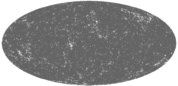
Figure 2:

Figure 3: