The early–type galaxy population in Abell 2218

Abstract

We present high signal-to-noise, moderate-resolution spectroscopy of 48 early-type members of the rich cluster Abell 2218 at $z=0.18$ taken with the LDSS2 spectrograph on the 4.2-m William Herschel Telescope. This sample is both larger and spans a wider galaxy luminosity range, down to $M^{\ast}_{B}+1$, than previous studies. In addition to the relatively large size of the sample we have detailed morphological information from archival Hubble Space Telescope imaging for 20 of the galaxies. We combine the morphological, photometric, kinematic and line-strength information to compare A 2218 with similar samples drawn from local clusters and to identify evolutionary changes between the samples which have occured over the last $\approx 3$ Gyrs. The overall picture is one of little or no evolution in nearly all galaxy parameters. Zeropoint offsets in the Faber–Jackson, Mg_b–$\sigma$ and Fundamental Plane relations are all consistent with passively evolving stellar populations. The slopes of these relations have not changed significantly in the 3 Gyrs between A 2218 and today. We do however find a significant spread in the estimated luminosity-weighted ages of the stellar populations in the galaxies, based on line diagnostic diagrams. This age spread is seen in both the disky early-type galaxies (S0) and also the ellipticals. We observe both ellipticals with a strong contribution from a young stellar population and lenticulars dominated by old stellar populations. On average, we find no evidence for systematic differences between the populations of ellipticals and lenticulars. In both cases there appears to be little evidence for differences between the stellar populations of the two samples. This points to a common formation epoch for the bulk of the stars in most of the early–type galaxies in A 2218. This result can be reconciled with the claims of rapid morphological evolution in distant clusters if the suggested transformation from spirals to lenticulars does not involve significant new star formation.

1 Introduction

The application of local galaxy scaling relations to the galaxy populations in distant clusters is widely regarded as one of the most powerful routes to understanding their formation and development. The main scaling relations which have been employed are the Faber–Jackson relation (FJR, luminosity–velocity dispersion, FJ76), the Kormendy relation (KR, surface brightness–effective radius, Korme77), the Fundamental Plane (FP, combining surface brightness, effective radius and velocity dispersion, DLBDFTW87,DD87,BBF92) and the Mg–velocity dispersion relation (Mg–$\sigma$, BBF93,CBDMSW99). These four relationships test different aspects of the luminosity and mass evolution of cluster galaxies and are predominantly applicable to the early-type galaxies which dominate the cores of rich clusters both locally and at high redshifts.

Two of these relations rely on accurate photometric and structural information for the galaxies, and as result there has been significant work employing WFPC2 on-board Hubble Space Telescope (HST ) to study the photometric evolution of morphologically-classified elliptical galaxies in distant clusters using the KR (BSL96; Schade et al. 1996, 1997; FCAF98,BASECDOPS98,ZSBBGS99). These studies suggest mild evolution in luminosity and size for ellipticals in rich clusters, consistent with passive evolution. Other groups assume “a priori” a degree of luminosity evolution based upon stellar population models and then attempt to use the observed KR evolution to constrain cosmological models [Pahre et al.1996, Moles et al.1998]. Unfortunately, as was pointed out by ZSBBGS99, the statistical and systematic errors in the measurement and transformation of HST magnitudes are too large to give unambigous results for cosmological parameters.

More detailed information comes from studies investigating the evolution of the FJR and FP which supplement the photometry (both HST and ground-based) with moderate-resolution spectroscopy, capable of resolving velocity dispersions down to $\approx 100$ km s^-1. Results have so far been published on the clusters A 2218 ($z=0.17$) and A 665 ($z=0.18$) by JFHD99; MS 1358$+$62 ($z=0.33$) and MS 2053–04 ($z=0.58$) by KDFIF97; A 370, MS 1512$+$36 and Cl 0949$+$44 all at $z=0.37$ (see BZB96,ZB97,BSZBBGH97b); Cl 0024$+$16 ($z=0.39$) by DF96, and MS 1054–03 ($z=0.83$) by DFKI98. In particular, the study of KIDF00 exploited a mosaic of HST images and Keck spectroscopy, to construct the FP for 30 luminous E and S0 galaxies in Cl 1358$+$62. The shape of the FP is very similar to that of the local Coma cluster and the offset between them can be explained by a mild evolution in luminosity. Unfortunately line strengths could not be explored since the widely-used Mg_b index falls into a strong telluric band at the cluster redshift. The combined data from all these studies strongly favour passive evolution of the stellar populations of early-type cluster galaxies both in surface brightness and mass-to-light ratio and a high redshift of formation, $z>2$. Further support for a high formation epoch for the stellar populations in early-type cluster galaxies comes from the modest evolution in the Mg_b absorption at a constant velocity dispersion in galaxies out to $z=0.37$ [Ziegler & Bender1997].

The relatively modest evolution claimed for the early-type population in clusters is in strong contrast to the evolution seen in the morphological mix in these environments. In particular, the origin of the well-studied “Butcher-Oemler” effect [Butcher & Oemler1984] in a population of star-forming cluster galaxies with spiral morphologies is now well established [Couch et al.1994, Couch et al.1998]. More recently there have been claims of morphological evolution in some classes of early-type galaxies in rich clusters. HST images have revealed an increasing paucity of S0 (lenticular) galaxies with redshift [Dressler et al.1997]. While S0s form the dominant luminous galaxy population in local rich clusters, DOCSE97 found that only 10–20% of bright cluster galaxies are S0s in rich clusters at $z\approx 0.5$. They suggested that this strong increase to the present-day resulted from the gradual transformation of spiral galaxies, accreted from the surrounding field, into S0s [Poggianti et al.1999]. If this transformation is relatively rapid, $<2$–3 Gyrs, then some proportion of the S0 population may show signatures of this past star formation activity in terms of young stellar populations and blue colours. However, low resolution spectroscopic surveys have typically failed to find large populations of bright, blue S0s [Couch et al.1998]. Moreover, the S0 population as a whole ought to show a wider dispersion in age than the cluster ellipticals. However, photometric analysis of morphologically-classified samples of ellipticals and S0s in distant clusters shows them to be almost identical in their 4000Å break colours [Ellis et al.1997], and hence by implication their ages. Unfortunately, the degeneracy between age and metallicity in most observables based on integrated spectra (e.g. broad-band optical photometry) make these hypotheses difficult to test conclusively [Worthey1994].

To break the age–metallicity degeneracy a number of groups have tried to identify absorption lines which are predominantly sensitive to age, e.g. Balmer lines, or which depend strongly on metallicity, mostly combinations of metal lines, [Jones & Worthey1995, Casuso et al.1996, Worthey & Ottaviani1997, Vazdekis & Arimoto1999]. Good progress has been made and we can now construct line diagnostic diagrams in which the age–metallicity degeneracy is nearly broken [Kuntschner & Davies1998, Jørgensen1999]. Recent analysis based on such line indices for the composite S0 populations in distant clusters have indicated that the stellar populations in luminous lenticular and elliptical cluster galaxies at $z=0.31$ have very similar luminosity-weighted mean ages [Jones, Smail & Couch2000]. This suggests that a model with a rapid transformation, from star-forming spiral to passive S0, is unlikely to be correct and a more gradual mechanism may be required [Poggianti et al.1999, Kodama & Smail2000].

Another approach to breaking the age–metallicity degeneracy is to use a combination of optical and optical-infrared photometry [Aaronson1978]. This approach has been used very recently by S00 to study the luminosity-weighted ages of early-type galaxies spanning a very wide range in luminosity in A 2218. This analysis suggests that while the most luminous ellipticals and S0s have very similar luminosity-weighted ages, the less luminous S0s may exhibit a much wider range in ages. Likewise, an intensive spectroscopic analysis of individual galaxies in the local Fornax poor cluster by Kunt00 has found that some of the lower luminosity S0 galaxies have extended star formation histories, compared to the more luminous ellipticals and S0s.

In the light of the discussion above, it is clearly important to apply the detailed spectroscopic techniques to individual galaxies spanning as wide a range in luminosity as possible in distant clusters, to study their line strengths and kinematics. However, this is very difficult and most previous spectroscopic studies have targetted only a modest number of typically the more luminous (and hence massive) galaxies in each cluster. We have therefore undertaken a programme to obtain high-quality spectra of a large number of early-type galaxies (of order 50) across a wide range of luminosity in two rich clusters A 2218 and A 2390. Both clusters have been imaged by HST providing accurate structural parameters. At $z=0.18$ and $z=0.23$ respectively, the cluster galaxies are bright enough to observe even sub-$L^{*}$ systems with 4-m class telescopes, while still representing a look-back time of around a quarter of the age of the Universe, adequate to address evolutionary questions. Both clusters are very rich systems and may well serve in the future as more suitable benchmarks for the comparison to very rich, high redshift clusters ($z\approx 1$) than Coma. Moreover, comparisons between A 2218 and A 2390 and more distant systems also have the advantage that aperture corrections are less important than for comparisons based on Coma.

In this paper, we present the study of galaxies in A 2218. In §2, the observations and the data reduction are described. Galaxy scaling relations and line diagnostic diagrams are examined in §3, and in §4 we discuss our results and give our conclusions in §5. The paper ends with comprehensive Appendices listing all our observational data.

Throughout the paper we adopt the following values for the cosmological parameters: $H_{0}=60$ km s^-1 Mpc^-1, $q_{0}=0.1$, $\Lambda=0$. For the nearby Coma comparison cluster ($z=0.024$) this results in a distance modulus of $dm=35.42$ mag and for A 2218 ($z=0.175$) in $dm=40.0$ mag, a scale of 3.51 kpc arcsec^-1 and a look–back time of 2.6 Gyrs.

2 Observations and data reduction

A 2218 is a very rich cluster at $z=0.18$ with a large velocity dispersion, $\sigma=1370^{+160}_{-120}$ km s^-1[Le Borgne et al.1992] and a high X-ray luminosity of $L_{X}$(0.5–4.4 keV) = $6.5\times 10^{44}$ ergs s^-1. An HST-based lensing analysis provides a detailed view of the mass distribution within the central 1 Mpc of the cluster and indicates a mass of $M(r<400{\rm kpc})=4\times 10^{14}M_{\odot}$ [Kneib et al.1996]. Most interestingly, the lensing map identifies two mass concentrations within the core of the cluster and led to the suggestion that it is suffering (or has just suffered) a core-penetrating merger.

A 2218 has previously been observed in a Fundamental Plane study by Jørgensen et al. (1999, JFHD). They targetted a sample of 11 early-type galaxies photometrically-selected from relatively shallow ground-based imaging. Their main conclusion was that both the evolution in luminosity, as well as in mass-to-light ratio, is modest and in agreement with passive stellar population models (e.g. BC93).

Our study of the early-type galaxy population in A 2218 is based upon optical photometry from the 5.1-m Hale telescope at Palomar Observatory and multi-object spectroscopy using LDSS2 at the 4.2-m William Herschel Telescope (WHT) on La Palma. In addition, we have exploited WFPC2 images taken with HST to provide high-quality morphological information for a subset of our sample. We next discuss the properties of these various datasets.

2.1 Hale/COSMIC imaging

The ground-based $UBVI$ imaging of a $9.7^{\prime}\times 9.7^{\prime}$ region centered on A 2218 (Fig. 9) used for our initial target selection was obtained with the COSMIC imaging spectrograph on the 5.1-m Hale telescope at Palomar during June 1994 and June 1995. A thick 2048² TEK CCD (pixel scale $0.286^{\prime\prime}$ pixel^-1) was used and individual exposures of $\sim 500$–1000 s were taken using in–field dithering (on a grid with $\sim 30^{\prime\prime}$ spacing). The frames were reduced in a standard manner with iraf using twilight flatfields to initially flatfield the frames before masking the brighter objects and stacking the data frames to create master flatfields in each filter. The data were then flatfielded using these master frames, aligned and coadded using a cosmic ray rejection algorithm. The total exposure times are 2.5 ks in $U$, 16.5 ks in $B$, 5.8 ks in $V$ and 21.7 ks in $I$ and the seeing measured on the final frames was 1.20^′′, 1.25^′′, 2.05^′′ and 0.95^′′ FWHM for $UBVI$ respectively. The frames were calibrated onto the Johnson/Cousins system of Lo92 and corrected for reddening calculated from the COBE dust maps [Schlegel et al.1998]. We estimate $E(B-V)=0.025$ leading to extinction coefficients for the Landolt filters of $A_{U}=0.136,A_{B}=0.108,A_{V}=0.083,A_{R}=0.067,A_{I}=0.048$ and $A_{702}=0.061$ for the HST/WFPC2 F702W filter. We determine $1\sigma$ limiting surface brightnesses of $\mu_{U}=26.1$, $\mu_{B}=28.9$, $\mu_{V}=28.0$ and $\mu_{I}=27.4$ mag arcsec^-2 for the final ground-based frames.

We used the SExtractor image analysis package [Bertin & Arnouts1996] to create a catalogue of galaxies detected in our deep $I$-band frame. We adopted a minimum area after convolution with a $0.86^{\prime\prime}$ FWHM top-hat filter of 0.82 sq. arcsec above the $\mu_{I}=24.6$ mag arcsec^-2 isophote. The galaxy catalogue created in this way includes positions, total magnitudes (mag_best from SExtractor) and crude morphological information on $\sim 2800$ stars and galaxies within the $I$-band frame. To calculate colours for these galaxies we measured aperture magnitudes within 4.0-^′′ (14 kpc) diameter apertures on the seeing-matched $UBVI$ frames and used these to construct $(U-B)$, $(B-V)$ and $(B-I)$ colours for the galaxies. In the Appendix we list the observed colours and coordinates for the galaxies we obtained spectra for (Table 4). The galaxy identifications are plotted on the full field in Fig. 9 and thumbnail images of the 48 galaxies are given in Fig. 10.

For the Faber–Jackson relation we translate our observed $I$-band magnitudes into absolute Gunn $r$ magnitudes, $r_{\rm abs}$, following the description of JFHD. The transformation of $I$ into restframe $r_{\rm rest}$ can be calculated with:

$$r_{\rm rest}=I+0.062(V-I)+0.76$$ (1)

Subtracting the distance modulus for A 2218 from $r_{\rm rest}$ then yields $r_{\rm abs}$. We use the extinction-corrected total $I$-band magnitudes ($I_{tot}$) and aperture $(V-I)$ colours in this calculation.

2.2 HST/WFPC2 imaging

In addition to the deep multi-colour ground-based imaging, morphological information is also available for a subset of the galaxies in our sample. This comes from an HST image of A 2218 taken with the WFPC2 camera on September 2, 1994. The total exposure time was 6.5 ks in the F702W filter ($R_{702}$) and the final frame covers a field of roughly $2.5^{\prime}\times 2.5^{\prime}$ at $\sim 0.15^{\prime\prime}$ resolution in the core of the cluster. These data were reduced and analysed by KESCS96 and more details can be found in that work.

The WFPC2 image has a $1\sigma$ surface brightness limit of $\mu_{R}\approx 30$ mag pixel^-2, which is more than adequate to provide high-quality morphological information on the brighter cluster members. Thumbnail images of the 19 galaxies (disregarding the cD) for which we have spectra are shown in Fig. 11 and we indicate the position of the HST field on Fig. 9. The brighter galaxies in the HST field ($R_{702}<22.5$) have been visually classified by Prof. W. Couch onto the revised Hubble scheme used by the MORPHS project (see S00).

2.2.1 Determination of structural parameters

To measure the structural parameters of the spectroscopically-observed early-type galaxies lying within the HST image (plus the cD galaxy) we extracted subframes of all 19 galaxies using midas and analysed each galaxy using the profile fitting method developed by Saglia et al. (1997a, 1997b). We briefly summarise this technique here: after masking stars and artifacts from around the galaxy, the circularly averaged surface brightness profile of the galaxy was fitted with PSF-convolved $r^{1/4}$ and exponential components (both simultaneously and separately). The PSF was generated using the tinytim software package [Krist & Hook1997]. The quality of the fits was assessed by Monte Carlo simulations, taking into account sky-subtraction corrections, signal-to-noise, the radial extent of the profiles and the $\chi^{2}$ quality of the fit. In this way, we were able to derive the effective radius ($r_{e}$ in arcsec), the total $F702W$-band magnitude ($R_{702}$) and the mean surface brightness within $r_{e}$ ($\langle\mu_{e}\rangle$) for the entire galaxy as well as the luminosity and scale of the bulge ($m_{b}$ and $r_{e,b}$) and disk ($m_{d}$ and $h$) component separately, within the limitations described by SBBBCDMW97. We estimate the average error in $R_{702}$ and $r_{e}$ to be $0.015$ mag and $25\%$ respectively. The structural parameters for all the galaxies can be found in Table 5 of the Appendix.

We also performed an isophote analysis based on the procedure introduced by BM87. Deviations from the elliptical isophotes were recorded as a function of radius by a Fourier decomposition algorithm. The presence and strength of the a4 coefficient (taken as a signature of diskyness) is in good agreement with the visually determined morphological class of S0 and early-type spirals.

2.2.2 Rest-Frame Surface Brightness Profiles

In order to determine the rest frame properties of the galaxies, we perform the transformation of the HST magnitudes to restframe Gunn $r_{rest}$ as described by JFHD. We summarize here the transformations introduced by JFHD: According to HBCHTWW95, the instrumental magnitude in the F702W filter is:

$$R_{702}=-2.5\log({\rm DN})/t_{{\rm exp}}+ZP+2.5\log(GR)$$ (2)

with $GR$ being the respective gain ratios for the WF chips and $ZP$ the zeropoint for an exposure time $t_{{\rm exp}}=1$ s. $ZP=21.670$ with consideration of the difference between “short” and “long” exposures of 0.05 mag [Hill et al.1998] and an aperture correction of 0.109 [Holtzman et al.1995]. This is transformed into Cousins $I$ using the equations

$$R_{c}=R_{702}+0.486(V-R_{c})-0.079(V-R_{c})^{2}$$ (3)

and

$$(V-R_{c})=0.52*(V-I)$$ (4)

which yields:

$$I=R_{702}-0.227(V-I)-0.021(V-I)^{2}$$ (5)

The $(V-I)$ colour was taken from our ground-based aperture photometry, see Table 4. The $4^{\prime\prime}$ photometric aperture yields an equivalent area for the distant galaxies to the area used in the Coma photometry. Finally, the calibration to restframe Gunn $r_{rest}$ is achieved using Equation 1.

Since the observed F702W passband is close to restframe Gunn $r_{rest}$ at the redshift of A 2218, the overall k-corrections are small. On average $R_{702}-r_{rest}=-0.40$. For the same reason, the effective radii can be directly compared to the ones measured of Coma galaxies in Gunn $r$. The mean surface brightness within $r_{e}$ is:

$$\langle\mu_{r}\rangle_{e}=r_{rest}+2.5\log(2\pi)+5\log(r_{e})-10\log(1+z)$$ (6)

where the last term corrects for the dimming due to the expansion of the Universe. The mean surface brightness in units of L_o/pc² is

$$\log\langle I\rangle_{e}=-0.4(\langle\mu_{r}\rangle_{e}-26.4)$$ (7)

With an angular distance of A 2218 of $d=683$ Mpc for our cosmology, the effective radius in kpc is:

$$\log(R_{e})=\log(r_{e})+\log(d)-2.314\quad(R_{e}\,\mbox{in kpc})$$ (8)

whereas Coma ($z=0.024$) has $d=115.7$ Mpc.

Compared to the data given by JFHD, our measurements are almost identical. For this comparison, we used only their HST-based sample. There are 15 galaxies in common with respect to the structural parameters and the largest deviations in $\langle\mu_{r}\rangle_{e}$ for these are only 3–6% in four galaxies (the cD and #1454, #1552 and #1662). These deviations may be due to residual background light from nearby bright galaxies (#1552 and #1662 are close to the cD, #1454 close to the giant elliptical #1437). For the remainder of the galaxies we summarize the comparison in Table 1. This table also contains the estimated total (random and systematic) errors of the parameters. While there are 15 galaxies between our sample and that from JFHD available to compare structural parameters, there are only six for which a similar spectroscopic comparison is possible.

Table 1: Difference between this paper and JFHD.

parameter	Ngal	Difference	error	errorJFHD
$R_{\mathrm{702}}$	11	$-$0.01$\pm$0.12	0.015	0.015
$(V-I)$	15	0.023$\pm$0.047	0.007	0.025
$r_{z}$	11	$-$0.03$\pm$0.11	0.05	0.05
$\log r_{e}$	11	0.003$\pm$0.071	0.111	0.078
$\langle\mu_{r}\rangle_{e}$	11	$-$0.00$\pm$0.24	0.25	0.29
$\log\sigma$	8	0.06$\pm$0.07	0.020	0.025

Errors are estimated total errors (random $+$ systematic).

2.3 WHT/LDSS2 multi–object spectroscopy

2.3.1 Sample Selection

The aim of the project is to study the stellar populations of a large sample of early-type cluster galaxies spanning a wide range in luminosity. However, owing to the need for good sky subtraction in our spectra we were constrained to include only around 20 galaxies in each mask. For this reason we took great care to select only galaxies which were likely to be cluster members based upon their broad-band colours from our ground-based $UBVI$ imaging.

Using the existing redshift catalogue for the field [Le Borgne et al.1992], we defined a region in $UBVI$ colour space which was occupied by cluster members. Galaxies falling outside the colour region, defined as $2.60<(B-I)<3.20$, $-0.50<(B-V)<0.50$ and $-0.10<(U-B)<0.50$, were rejected (see, e.g. Fig. 1). The width of this region places negligible restrictions on the stellar populations of the selected galaxies, but rejects the majority of background galaxies. Combined with the richness of the cluster this ensured a high rate of success in targetting cluster members in our spectroscopic sample (1 non-member out of 49 targets). The colour-selected sample of galaxies includes 138 galaxies with $I_{\rm tot}<18.8$ (our adopted magnitude limit) within the $9.7^{\prime}\times 9.7^{\prime}$ area covered by the Hale images.

This catalogue was then used as the input for mask design. We prepared two masks containing galaxies with an average $I$-band surface brightness within the spectroscopic slit brighter than $\mu_{I}=19.7$ mag arcsec^-2. A third mask contained galaxies as faint as $\mu_{I}=20.2$ mag arcsec^-2. Dividing the galaxies between the masks in this way enabled exposure times to be chosen to ensure that similar signal to noise was obtained in each spectrum.

The position angles of the masks were chosen so as to maximise the number of galaxies with early-type morphologies (E–S0–Sa) selected within the HST field. Galaxies were allocated to slits manually. With few exceptions, a minimum slit length of $15^{\prime\prime}$ was used, and the position of the slit was also chosen so that fainter companion galaxies did not obscure the sky. Occasionally, the choice of either of two galaxies made the packing of the mask equally efficient. In this situation, we preferred galaxies for which a redshift was already known.

Figure 1: The $(B-I)$–$I$ colour magnitude diagram from our Hale imaging for bright galaxies lying in a $9.7^{\prime}\times 9.7^{\prime}$ (2.2 Mpc) region centered on A 2218. The sequence of red cluster members is readily seen extending down to $I\sim 22$ ($M_{B}\sim-17$). The box encompasses galaxies matching our selection criteria, while circles denote those galaxies which were actually observed.

2.3.2 Observations

During the nights of June 2–5, 1997, we obtained multi-object spectroscopy using LDSS2 [Allington-Smith et al.1994] at the WHT. To obtain high-quality spectra for the faint galaxies in A 2218 at $z=0.18$, we designed a new high dispersion grism optimised for red wavelengths. The existing LDSS2 high-dispersion blue grism has relatively low throughput in the wavelength range of interest here ($\lambda\lambda=6000$–7000Å). More critically, the undeviated central wavelength of this grism is 4200Å, this severely limits the field of view that can be obtained because of the large deviation of the redder wavelengths which cause them to fall at the extreme edge of the detector.

The new high-dispersion red grism, R640, consists of a 600 l/mm, $34^{\circ}$-blaze angle transmission grating coupled to a $32.7^{\circ}$ Schott SF10 high refractive index prism. This combination achieves an undeviated central wavelength of 6500Å allowing the whole of the field-of-view to be used to select galaxies. The intrinsic dispersion of the SF10 glass also helps boost the dispersion of the grism by $\approx$8% providing a measured dispersion of 2.1Å per pixel with the SITe CCD (24$\mu$m pixels, spatial resolution $0.59^{\prime\prime}$ pixel^-1). The peak efficiency of the grism, $\approx 55\%$, represents a gain of almost a factor of two in the $\lambda\lambda=6000$–7000Å region over that available from the high-dispersion blue grism.

With a slit width of $1.5^{\prime\prime}$ the R640 grism provides a limiting spectral resolution element of 4.6Å FWHM. This allows us to measure velocity dispersions for galaxies as low as $\approx 120$ km s^-1, at which point, the intrinsic and instrumental broadening of the spectra are equal. Observing with the S1 3750 blocking filter the total restframe wavelength range covered by the SITe CCD was $\lambda\lambda\approx 4900-6400$Å encompassing the important absorption lines H$\gamma$, H$\beta$, Mg_b and Fe5270 at the cluster redshift.

The three masks were observed with total exposure times of about 5 hours each (Table 2). Of the 61 galaxy spectra, 12 galaxies were included on two different masks to allow us to check for systematic variations between the results from the various masks. There is only one foreground galaxy (#2302, only 10,000 km s^-1 away from A 2218) which demonstrates the efficiency of our sample selection. In total therefore we obtained spectra of 48 different cluster galaxies, of which 19 lie within the HST image. They were morphologically classified visually by Prof. W. Couch, who classifies them as 8 E, 1 E/S0, 5 S0, 3 SB0/a, 1 Sa, 1 Sab (see Table 5), hence galaxies with disks make up 50% of our HST sample. In addition five of the galaxies outside the HST field have clear evidence for a disk component (see Table 6), but the modest seeing ($0.95^{\prime\prime}$ in $I$) of our ground-based images prevents us from classifying them in more detail.

Table 2: Observation of the masks.

Mask	number of galaxies	$t_{\mathrm{exp}}$ [hr]
2	24	5.50
5	19	4.75
7	18	4.50

2.3.3 Reduction and analysis of the spectra

The spectral reduction was undertaken using midas with own fortran routines and followed the standard procedure, including correction for S–distortions of the spectra closest to the edges of the field. The individual 2-d images of the slitlets were extracted from the whole frame (after bias subtraction) and reduced individually. Dome flat–fields were used to correct for pixel-to-pixel variation, cosmic rays were removed by a $\kappa$–$\sigma$ clipping algorithm with a $5\times 5$ pixel filter and bad columns were cleaned by interpolating adjacent columns (there were 0 to 5 bad columns per slitlet). The rectification was achieved by tracing the spectral profiles and then shifting the pixels in the spatial direction. This transformation was applied in the same manner to the science, calibration and sky flat images. After sky flat–fielding, to correct for illumination effects, the spectra were wavelength calibrated and the sky was subtracted by modeling each CCD column seperately. One-dimensional spectra were extracted using the Horne–algorithm [Horne1986], which optimally weights the extracted profile to maximise the signal-to-noise. Finally, the one-dimensional spectra were rebinned to logarithmic wavelength steps in preparation for the Fourier Correlation Quotient (FCQ) determination of the velocity dispersion and the measurement of absorption line strengths.

Spectra of standard stars were reduced in a similar manner. A spectrophotometric flux standard (BD$+$28 4211) was observed through an acquisition star hole in one mask. Template G and K giants stars (HD 102494, HD 107328, HD 126778, HD 132737 and HD 184275) were observed through a longslit using the same grism as for the galaxies. To minimize the effect of the possible variation in slit width the star spectra were summed over a small number of rows.

The velocity dispersions (as well as the radial velocities) were determined using the latest version of the FCQ program kindly provided by Prof. R. Bender (see Bende90a). The wavelength range analyzed ($\lambda\lambda=5943$–6279Å) was centered on the Mg_b feature and lies between two very strong telluric emission lines. The resulting dispersions cannot be interpreted simply, since the slitlets had small variations in width and were therefore not identical in width to the longslit. We applied a procedure to corrrect for this. FCQ was run on all galaxies to give a $\sigma_{{\rm fcq}}$ for each of the five template stars. Separately we computed the width of the auto-correlation function of each star, $\sigma_{\rm star}$, and added this in quadrature to estimate the total line width of the galaxy absorption lines using each template : $\sigma_{{\rm tot}}=\sqrt{\sigma_{{\rm fcq}}^{2}+\sigma_{{\rm star}}^{2}}$. We determined the final value of the stellar velocity dispersion by taking the median value of these five measurements, $\overline{\sigma_{\rm tot}}$, and subtracting from it (in quadrature) the instrumental dispersion, $\sigma_{{\rm inst}}$ i.e.  $\sigma_{\rm gal}=\sqrt{\overline{\sigma_{\rm tot}}^{2}-{\sigma_{\rm inst}}^{2}}$. The instrumental dispersion is determined using eight unblended emission lines in the arc spectrum, from the appropriate slitlet, to evaluate the width of an arc line at the position of Mg_b in the redshifted galaxy spectrum. All the values of $\sigma_{{\rm gal}}$ are given in Table 6 together with the heliocentric radial velocities $v_{{\rm rad}}$.

For comparison, velocity dispersions of all galaxies of one mask were also measured using the iraf package fxcor yielding an average difference of only 28 km s^-1. We also compare our velocity dispersion results with those of early-type galaxies in common with JFHD (see Table 3). The median difference in $\sigma_{{\rm gal}}$ is 22 km s^-1 or 10%.

Table 3: Comparison between our measurements and JFHD.

Galaxy	$v_{{\rm rad}}$	$v_{{\rm JFHD}}$	$\Delta v$	$\sigma_{{\rm gal}}$	$\sigma_{{\rm JFHD}}$	$\Delta\sigma$
1293	47895.8	47882.5	13.3	239.9	201.4	38.5
1343	50026.9	49986.2	40.7	241.5	248.3	$-$6.8
1437	48495.0	48478.5	16.5	248.5	204.6	43.8
1662	44948.2	44928.6	19.5	364.9	298.5	66.4
1711	47619.0	47608.8	10.2	203.7	215.3	$-$11.6
1914	47555.5	47534.1	21.4	147.4	162.2	$-$14.7
2076	49399.4	49394.3	5.1	219.0	196.8	22.2
2604	49390.2	49418.9	$-$28.8	187.8	130.9	56.8

Galaxy numbers correspond to those in Table 6, $v_{{\rm rad}}$ heliocentric radial velocity measured by us, $v_{{\rm JFHD}}$ heliocentric radial velocity measured by JFHD, $\Delta v$ the difference between both measurements. $\sigma_{{\rm gal}}$: velocity dispersion measured by us and corrected to the same aperture used by JFHD, $\sigma_{{\rm JFHD}}$: velocity dispersion measured by JFHD, $\Delta\sigma$ the difference between both measurements. All velocities are in km s^-1.

The absorption indices were measured on the Lick system [Faber et al.1985]. Our spectra were first degraded to the resolution of the Lick system. The indices were then corrected for the velocity broadening $\sigma_{{\rm gal}}$ (a few example spectra are shown in Fig. 12). Because the equivalent widths are determined with respect to a local continuum, flux calibration has little effect on the (atomic) absorption line strengths (the average difference in Mg_b for example is $-0.014$Å, which is about 10% of the typical error). Nevertheless, we present in Table 6 the line strengths of H$\beta$ and Mg_b measured from the flux-calibrated spectra (values of other indices may be requested from the first author). We calibrated the data using standard stars in common with the EFAR studies [Colless et al.1999]. These showed a scatter around zero with $\sigma=\pm 0.1$Å for Mg_b and hence no recalibration was applied to the index strengths to place them on the Lick system.

The absorption of the iron lines Fe5270 and Fe5335 could not be derived reliably for the majority of the galaxies because the red continuum band of Fe5270 is contaminated the [OI] telluric emission line at $\lambda=6296$Å. The Fe5335 line is also redshifted into this sky line, so that this absorption feature cannot be measured. The same problem also arises for the red continuum window of Mg₂.

From the repeat observation of 12 galaxies on different masks we are able to confirm the internal reliability of our spectral analysis. As an example we show two independent spectra of galaxy #786 in Fig. 2, indicating that the continuum as well as the H$\beta$ and Mg_b indices are well matched. If we take all 12 comparison spectra regardless of their signal-to-noise we find median offsets for the H$\beta$ and Mg_b line indices and velocity dispersion, $\sigma$, at the $<10$% level.

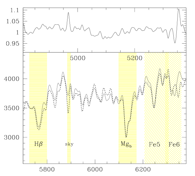
Figure 2: Lower panel: Flux-calibrated spectra of galaxy #786 observed through two different masks. The spectra have been degraded to the Lick resolution and normalized at Mg_b. Index definitions are overplotted as hatched areas (Fe5=Fe5270, Fe6=Fe5335). The continuum as well as the H$\beta$ and Mg_b indices are all well matched. Only the Fe5335 index is severely affected by two sky emission lines. The lower axis represents observed wavelengths, the upper shows restframe wavelengths (in Å). (See also Fig. 12). The abscissa is in counts (1 ADU $=1.3e^{-}$). Upper panel: ratio of the 2 spectra.

3 The Local Comparison Sample

3.1 Photometry and Structural Parameters

The Coma cluster provides a good local reference as it represents the best studied rich local cluster, albeit less rich than A 2218. We take data on early-type galaxies in the cluster from Joerg99 and JFK95b. Their galaxy photometry was taken through the Gunn $r$ filter, then corrected for extinction and cosmic expansion. The combined sample contains 115 early-type galaxies (35 E, 55 S0, 25 intermediate types) and is 93 % complete at absolute magnitudes $M_{r}<-20.35$.

3.2 Velocity Dispersions

The spectroscopic data in Joerg99 and JFK95 were aperture corrected by the authors to match a circular aperture with radius 1.7^′′. Therefore, we corrected our velocity dispersion ($\sigma$) determinations by $\Delta(\log\sigma)=+0.025$ to match the Coma aperture. The aperture correction was computed from the logarithmic gradient given by JFK95:

$$\Delta(\log\sigma)=0.04\cdot\log\left(\frac{d({\rm A\,2218})}{d({\rm Coma})}\cdot\frac{a({\rm A\,2218})}{a({\rm Coma})}\right)$$ (9)

where $d$ is the angular distance and $a$ is the aperture radius. For our observations $a$ was taken as the harmonic mean of the slit width of 1.7^′′ and the weighted number of rows (an average of 4.7 pixels, or 2.8^′′) over which the spectra were integrated by the Horne algorithm.

3.3 Line Indices

The best available sample of line indices for local early-type galaxies comes from the SMAC collaboration [Kuntschner et al.2000]. We use this dataset therefore as the primary comparison source for our line index analyses. While the SMAC sample includes galaxies from lower density regions (such as the Virgo cluster), about half of the dataset comes from the Coma cluster. We chose not to use line indices from Joerg99 because the H$\beta$ absorption strengths are not compatible with the higher S/N observations of KLSHD00 (see Fig. 1 of that paper).

The Mg equivalent widths of the A 2218 galaxies were aperture corrected according to the same prescription given by JFK95 as for the velocity dispersions. For the conversion between Mg₂ and Mg_b we follow ZB97 and adopt a factor of 15. This leads to a coefficient of 0.6 (instead of 0.04) in Eq. 9 resulting in a mean aperture correction of $\Delta({\rm Mg}_{b})=+0.37$Å for the A 2218 galaxies. We did not correct the H$\beta$ line strengths for aperture effects since no significant radial dependence of this index is found in local galaxies [Mehlert et al.2000].

4 Results

4.1 Comparison with local data

We begin by explaining the symbols used in the figures on which the following discussion is based. In all subsequent figures, large symbols are galaxies in A 2218, while small boxes represent the local reference sample. Galaxies classified morphologically as S0 or early-type spiral galaxies (from the A 2218 HST field) as well as five galaxies that clearly exhibit disks in the ground-based images are shown by filled symbols. In Section 4.3, we will divide the full A 2218 sample radially into two subsamples with equal numbers of galaxies. The core region (all galaxies within 130″ from the cluster centre) overlaps with the HST field (providing morphological classifications) and we show these galaxies as circles. Galaxies in the outer region (triangles) may contain small disks which can not be detected on the ground-based images. We fit both the distant and the local sample only within the region shown by horizontal and/or vertical dotted lines in the plots, which represent the selection boundaries for the A 2218 data.

For linear fits to the relations we use the bisector method, which is a combination of two least-square fits with the dependent and independent variable interchanged. Errors on the bisector fits were determined by bootstrap resampling the data 100 times. The shaded area in each figure illustrates the possible slopes within the $\pm 1\sigma$ bounds on the mean slope of the A 2218 sample, whereas the two solid lines indicate the same range for the local comparison data. All fit results are given in Table 7 in the Appendix.

4.1.1 Faber–Jackson relation

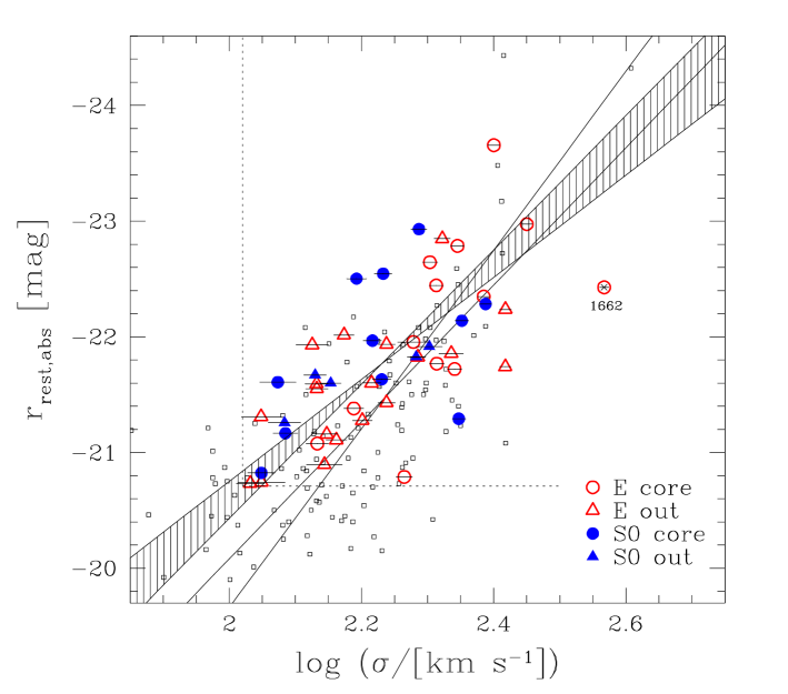
Figure 3: The Faber–Jackson relation (velocity dispersion versus total restframe Gunn $r$ magnitude) for the galaxies in A 2218 (large symbols), compared to Coma early-type galaxies (small open boxes; Jørgensen et al. 1995, 1999). Hashed area: fits to the distant FJR (within $\pm 1\sigma$), open area: fits to the local FJR within selection boundaries of the distant sample (dotted lines).

The Faber–Jackson relation in A 2218 is compared to the Coma sample of Jørgensen et al. (1995b) in Fig. 3. Due to the lookback time to A 2218, we should expect galaxies in this cluster to be brighter than their counterparts in Coma at a given velocity dispersion. If we assume that cluster galaxies are formed at $z_{f}=2$, passive evolution would increase their brightness by $0.19$ mag [Bruzual & Charlot1993]. The observed change in absolute magnitude is $0.30\pm 0.09$ mag, which is compatible with the theoretical prediction.

With 48 galaxies in A 2218 covering velocity dispersions down to $105$ km s^-1, we are also able to investigate the evolution in the slope of the FJR. The slope of the Coma data is steeper than that in A 2218 (a difference of $1.7\pm 1.1$) but the offset has low statistical significance, and depends on the boundaries used to define the Coma galaxy sample. Thus there is only weak evidence from this plot for differential evolution of massive and less-massive early-type galaxies. It is worth noting, however, that the A 2218 data may also have larger scatter than that of the Coma sample. This may indicate a wider range of recent star formation histories of galaxies in the A 2218 cluster, an issue to which we will return in the following sections.

Looking at the individual galaxies in A 2218, one in particular stands out: #1662 (marked with a cross in Fig. 3). This galaxy has a higher velocity dispersion than the cD galaxy (as measured by JFHD), it is located close to the cD and shows moderately high ellipticity, a positive a4 coefficient and some asymmetry in the HST image (see Fig. 11). We confirmed that there was no other galaxies on the slit and splitting the spectroscopic exposures into two independent halves we find roughly equal and high $\sigma$’s. The origin of this galaxy is puzzling: it could perhaps be the stripped core of a massive galaxy, although it is hard to understand why the parent galaxy would have been susceptible to stripping if it were as large as suggested by the dispersion.

4.1.2 Line index analysis

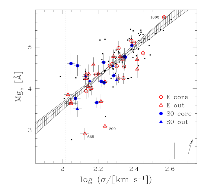
Figure 4: Mg_b–$\sigma$ relation of A 2218 compared to the SMAC sample (small filled boxes). Symbols and lines as in Fig. 3. The arrow in the lower right corner shows the aperture correction applied to the measured $\sigma$ and Mg_b of the distant galaxies, the cross represents the median errors for the SMAC data (Kuntschner et al. 2000).

Overall, the distribution of A 2218 galaxies in the Mg_b–$\sigma$ plane is quite similar to that of local early–type galaxies in the SMAC sample (see Fig. 4). However, two galaxies in A 2218 (#299 and #665) stand out as peculiar, having low Mg_b line strengths for their $\sigma$’s. #299 has a strong H$\beta$ absorption so that it may be a post-starburst (k+a or E$+$A) galaxy, while #665 has an average H$\beta$ value. It is not possible to detect any stellar disk in either #299 or #665 in the ground–based images, but both galaxies are very blue in ($U-V$) compared to the luminosity-corrected mean colour–magnitude relation of the total sample (this is also true for #704 and #1605 which have high H$\beta$ absorption) perhaps indicating some recent star formation activity. The galaxy with the highest $\sigma$ (#1662, marked with a cross in Fig. 4) has a Mg_b line strength which is compatible with the Mg_b–$\sigma$ relation of the other A 2218 galaxies.

Whether or not we excluded the galaxies #299 and #665 from the bootstrap bisector fits, the slopes for the A 2218 and local samples are consistent ($\Delta\hbox{slope}=0.18\pm 0.58$ with these galaxies included; $\Delta\hbox{slope}=-0.26\pm 0.48$ with these galaxies excluded). The offset between the two samples is more dependent on whether these galaxies are included, since they tend to reduce the average Mg_b absorption ($\Delta\hbox{zp}=-0.061\pm 0.074$Å with the galaxies included; $\Delta\hbox{zp}=-0.004\pm 0.072$Å with the galaxies excluded).

We can compare this shift with that expected due to the passive evolution of the galaxy population by adopting a formation redshift. For $z_{f}=2$, we expect a change $\Delta\hbox{zp}=-0.19$Å (assuming a typical [Fe/H] of 0.25 for the sample, see ZB97). Since we see a significantly smaller offset, the average galaxy must have been formed at a considerably earlier time. However, if we exclude the galaxies #299 and #665 we may well be removing exactly those galaxies which are showing evolutionary differences. Including these galaxies and allowing for a systematic offset of 0.1 in the relative calibration of the spectral index would reduce the difference to within the statistical uncertainty of our fiducial model.

Since the H$\beta$ line index is more age sensitive, but less dependent on metallicity than Mg_b, we explore the age/metallicity spread of the A 2218 galaxies in more detail in Figs. 5 and 6. The distribution within the H$\beta$–$\sigma$ plane is broad. In particular, the large scatter of the fainter galaxies in H$\beta$ indicates a wide range of star formation histories. The more massive galaxies in A 2218 have on average higher H$\beta$ absorption than galaxies in the SMAC sample with the same velocity dispersion. This is illustrated in Figs. 5 by calculating the median H$\beta$ aborption in five bins (medians for each sample are indicated by solid and dotted horizontal bars respectively in Fig. 5). Although there is a trend for $H\beta$ to increase with decreasing velocity dispersion, this effect is complicated by the systematic variation in metal abundance with velocity dispersion. We return to this issue below, and firstly concentrate on the offset of the brighter galaxies. Comparing the four brightest bins, the offset is $\approx 0.35\pm 0.1$Å. We are confident that this systematic offset cannot be produced by calibration errors since our systematic errors are less than 0.1Å.

In order to interpret this difference, we compare the absolute values of the H$\beta$ index with the Worthey model (1994), and also in a relative sense only. The absolute values of the index suggests that galaxies in the SMAC sample have luminosity weighted ages for their stellar populations of 8 Gyr, hile A 2218 galaxies are much younger, with luminosity weighted ages of only 4 Gyr (compare with Fig. 6). However, the absolute calibration of the model is uncertain. A more reliable approach is to compare the difference in absorption line strength with that expected from the difference in lookback time. The expected difference in H$\beta$ line strength for a single population formed at $z_{f}=2$, observed at $z=0.17$ and the present day is 0.14 Å. This is less than the observed shift, although the two values could be reconciled if we include both the maximum systematic uncertainty of 0.1 Å in the index calibration and the statistical uncertainty. Nevertheless, it is interesting to note that the pressure from the H$\beta$ index is to introduce more recent star formation, while the pressure from the Mg_b observations is to make the galaxies older. It is unlikely that this conflict arises from our use of a single age stellar population to interpret the differences as the intermediate age population will have similar effects on both indices.

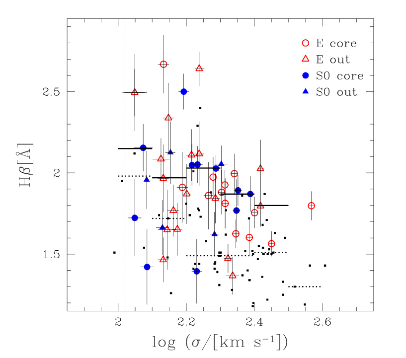
Figure 5: The distribution of the H$\beta$ line indices of the A 2218 early–type galaxies compared to SMAC. Symbols as in Fig. 3. Short horizontal solid lines: median value of H$\beta$ for specific $\sigma$ bins for A 2218; horizontal dotted lines: same for SMAC.

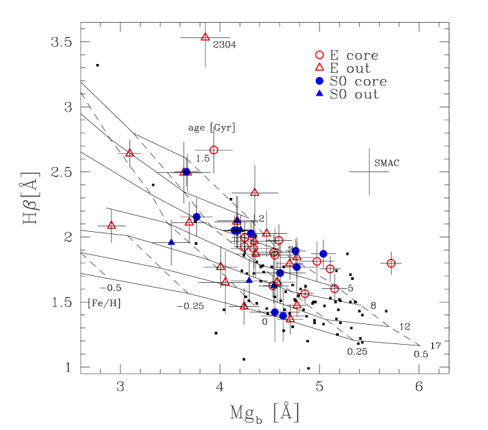
Figure 6: Age – metallicity diagnostic diagram using H$\beta$ as a primary age indicator and Mg_b as a metallicity indicator. Big symbols: A 2218, small filled boxes: SMAC sample (Kuntschner et al. 2000, typical errorbar shown). Overplotted is a grid of SSP models from Worthey (1994) shifted as described in the text. “Horizontal” lines follow constant age, “vertical” lines constant metallicity.

Exploring the distribution of A 2218 galaxies between age and metallicity using line diagnostic diagrams has the advantage over the Mg_b–$\sigma$ and H$\beta$–$\sigma$ diagrams, in that it does not rely on assuming a universal metal abundance – velocity dispersion relation before we can extract any information on the ages of the stellar populations. We use the Mg_b–H$\beta$ diagram, Fig. 6, rather than the combined [MgFe] index, because we were unable to derive reliable Fe indices for all our galaxies. The Mg_b–H$\beta$ correlation has the drawback that the models based on solar abundance ratios do not match the Mg/Fe ratio observed in early-type galaxies [Thomas et al.1999]. However, we are primarily interested in the relative ages of galaxies, so we can apply an empirical relationship between Mg_b and [MgFe] from the SMAC data to the model grid of Worth94: Mg_b$=$[MgFe]$*1.58-1.20$, to transform it to the relevant observables. While ages derived from this grid are clearly uncertain in an absolute sense, this approach allows us to quantify the relative offsets between the data.

The bulk of the A 2218 galaxy population show systematically younger ages at a fixed metallicity compared to the SMAC galaxies (Fig. 6). This contributes to a deficit of A 2218 galaxies in the lower right-hand corner of the plot compared to the SMAC sample. There is also a systematic shift between the two samples that is driven by the H$\beta$ index. The magnitude of the offset is larger than that expected for the look-back time to A 2218 if the galaxies form all their stars at redshifts above 2, as we have discussed previously. Since the velocity dispersions of the galaxies are not directly visible in this diagram, the comparison suggests that the evolution of Mg_b and H$\beta$ are consistent; it only becomes evident from comparing the distribution of galaxies in Figures 4 and 5 that the SMAC sample contains a higher proportion of high velocity dispersion galaxies. Thus, while galaxies in A 2218 occupy a large region of the available parameter space in Fig. 6 and appear to be more diverse than the SMAC population, the result is not conclusive because low $\sigma$ galaxies, which in general show a wider range in H$\beta$, are under-represented in the SMAC sample.

A few galaxies in A 2218 are exceptions to the general distribution, having H$\beta$ as low as galaxies in the SMAC dataset. We have searched for emission in these galaxies, which might fill-in the H$\beta$ line, but find none. In contrast, galaxy #2304 has very strong Balmer absorption in H$\beta$ and also in the H$\gamma$ and H$\gamma_{A}$ indices. This galaxy has clearly undergone a starburst in the recent past, and is an example of the post-starburst galaxies frequently identified in lower-resolution studies of more distant clusters (e.g. PSDCB99).

4.1.3 Fundamental Plane

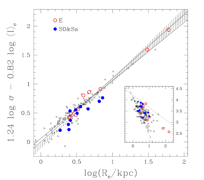
Figure 7: The Fundamental Plane of A 2218 early-type galaxies (big symbols) compared to Coma (small open boxes, Jørgensen et al. 1995a; Jørgensen 1999). Lines as in Fig. 3. The HST F702W photometry was transformed to restframe Gunn $r_{rest}$ magnitudes as described in Section 2.2.2. The full diagram shows the edge-on view, while the inset shows the FP face-on (using the same symbols). The abscissa is $(2.21\log(R_{e})-0.82\log\langle I\rangle_{e}+1.24\log\sigma)/2.66$, ordinate $(1.24\log\langle I\rangle_{e}+0.82\log\sigma)/1.49$. The dotted line indicates the “exclusion zone” for nearby galaxies, the dashed line the magnitude completeness limit for the Coma sample.

Another probe of the star formation histories of galaxies is the stellar mass-to-light ratio. We can investigate the Fundamental Plane (FP) of A 2218, restricting the analysis to those galaxies within the HST field where accurate measurements of the structural parameters are possible. In Fig. 7, we present the FP and compare the distant galaxies to the Coma sample of Jørgensen et al. (1995a, 1996). The scatter around the FP of A 2218 is with 0.108 in $\log(R_{e})$. This is very similar to the scatter seen in Coma, 0.096, as is the distribution of the galaxies across the surface of the plane (inset panel in Fig. 7). The average brightening of the A 2218 early-type galaxies can be investigated by assuming that there is no evolution in the structure of the galaxies (i.e. $R_{e}$ and $\sigma$ remain fixed). In this case the evolution of the zero-point of the relation measures the increase in brightness. The zero-point offset is $0.067\pm 0.023$ mag, consistent with a $z_{f}=2$ passive evolution model which predicts a shift of 0.10 mag.

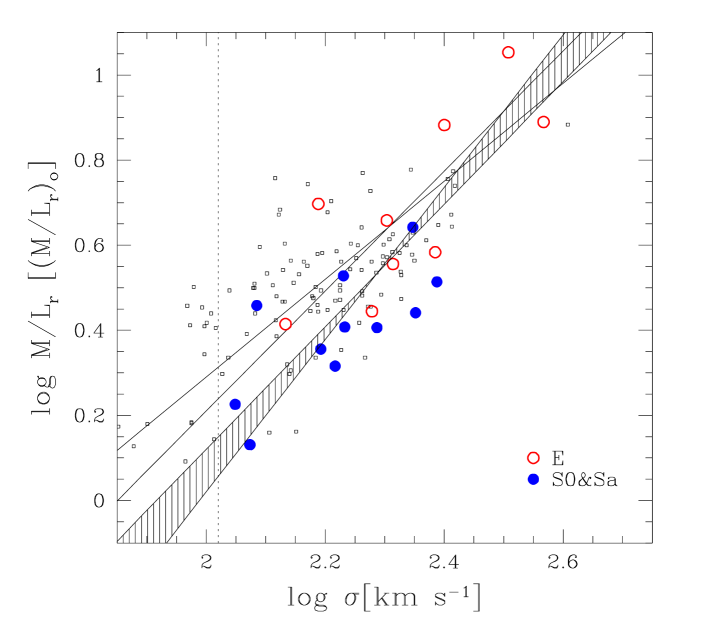
Figure 8: The mass-to-light ratio versus velocity dispersion. Symbols as in Fig. 7. Hashed area: fits to the A 2218 galaxies (within $\pm 1\sigma$), open area: fits to the Coma sample within selection boundaries of the distant sample (dotted line).

To cast this discussion in terms of mass-to-light ratios (Fig. 8) we calculated the masses of the galaxies following JFHD: $M=5R_{e}\sigma^{2}/G$, based on BBF92. We limited the Coma sample to galaxies with $\log\sigma\geq 2.02$ (dotted line in Fig. 8) in order to match the area of parameter space covered by the A 2218 galaxies. The bootstrap bisector fits to $M/L=a\sigma^{m}$ show compatible M/L slopes ($\Delta m=0.34\pm 0.20$) but a systematic offset in the zero point of the relation, $\Delta a=0.080\pm 0.026$. This is consistent with the expected change due to passive evolution: $\Delta a=0.12$.

In their $M/L$ analysis, JFHD find a substantial evolution in the slope of this relation. While their Coma value ($m=0.66\pm 0.13$) is much flatter than the slope for their five intermediate redshift clusters ($m=1.49\pm 0.29$ including A 2218), the slopes we determine for Coma and A 2218 are both compatible (and similar to that found for their intermediate redshift clusters by JFHD). The difference between our estimate of the Coma slope and that from JFHD must result from the different fitting methods applied, in particular our exclusion of the lowest velocity dispersion galaxies.

Finally, we note that we have searched for a trend in H$\beta$ line strength with M/L, but did not find one. Thus the naive expectation that a recent star formation event would equally effect a galaxy’s brightness and its Balmer line strength is not apparent in our dataset.

4.1.4 Summary and Discussion

The overall result from the comparison of bright galaxies in A 2218 and the local reference cluster, Coma, is that the galaxy population has evolved little between $z=0.18$ and the present-day. This is consistent with an early formation epoch for the bulk of their stellar populations. The distribution of the galaxies in the Mg_b–$\sigma$ plane and on the Faber–Jackson relation is almost identical in the two clusters. Weak evolution of bright galaxies in clusters sets strong limits on their formation epoch, as has been discussed extensively for the Mg–$\sigma$ relation [Ziegler & Bender1997] and the Fundamental Plane at intermediate redshifts (e.g. BSZBBGH97b,JFHD99), and even out to $z\sim 1$ (e.g. DFKI98). The changes we see in the dynamical relations for bright galaxies reinforces the conclusions of these authors. However, we are also in a position to address the ages of stellar populations directly using the age sensitive H$\beta$ line index.

In the H$\beta$–$\sigma$ diagram (Fig 5), the distant galaxies cover a wide range in H$\beta$, indicative of differences in the stellar populations. The low-dispersion galaxies have the greatest range of H$\beta$ line strengths. Some of these galaxies clearly had extended star formation activity at a low level, or recent episodes of minor star formation involving a few per cent of the total mass. Although the expected increase in luminosity is less visible in the FJ and FP relations, this is in line with the study of ZSBBGS99. These authors have investigated the Kormendy relation (the photometric projection of the FP) of five distant clusters and concluded that current accuracy of photometric data (even from HST) is not high enough to exclude low-level star formation activity in early–type galaxies.

Comparing the H$\beta$–Mg_b measurements to models, we find that the bulk of A 2218 galaxies have younger luminosity-weighted ages than nearby galaxies, as expected from the look-back time to $z=0.18$. The lower luminosity galaxies exhibit a wider range of stellar ages and metallicities. This tendency for lower luminosity galaxies to be less homogeneous is consistent with the expectation of models of the Butcher-Oemler effect in distant clusters [Smail et al.1998, Poggianti et al.1999, Kodama & Bower 2000, Smail et al.2001]. In the scenarios presented by these authors, the blue, star-forming galaxies responsible for the Butcher-Oemler effect are expected to undergo significant fading of their stellar populations when star formation ceases, as well as perhaps suffering more active stripping of stars by dynamical processes within the clusters [Smail et al.1998, Poggianti et al.1999]. For these reasons the evolved descendents of the Butcher-Oemler galaxies will on average be found in the lower luminosity galaxy population at lower redshifts. Equivalently, the lower luminosity galaxies will show a wider range in their previous star formation histories and our observations tend to support this suggestion.

4.2 E vs S0 Comparison

Based on morphologies determined from HST/WFPC2 images, DOCSE97 have shown that distant rich clusters contain a greater fraction of spiral galaxies, and a correspondingly smaller fraction of S0 galaxies, than similar local clusters. Over the redshift range 0–0.5, the S0 fraction decreases from 60% locally to 10–20% in the higher redshift clusters. In contrast, it appears that the elliptical galaxy fraction remained relatively constant over the last 5 Gyrs. The different evolutionary histories of these populations might be detectable at $z\approx 0.2$, even though the properties of E and S0 galaxies are very similar in the nearby Universe (e.g. BBF92,BBF93,SBD93). In an attempt to uncover such evidence, JSC00 have analysed the combined spectra of E and S0 galaxies in three clusters at $z=0.31$. Surprisingly they found no significant difference between the stellar populations in the two classes of galaxies. We repeat this test here, exploiting the fact that our spectra have higher signal-to-noise allowing us to search for differences between individual galaxies, rather than having to look at the average galaxy population.

In Figs. 3–8, we have distinguished between elliptical galaxies and those that have been morphologically classified as S0 or early–type spirals from the HST imaging (see Table 5) or which show a strong disk component clearly visible in the ground-based images (see Table 6). We will now discuss the differences between these two populations (in the following refered to as ‘ellipticals’ or Es and ‘lenticulars’ or S0s, respectively) as exhibited in those figures.

4.2.1 Faber–Jackson relation

We begin by comparing the FJR (Fig. 3). Since the E and S0 sub-samples have similar distributions in $\log\sigma$, the two-dimensional Kolmogorov–Smirnov test provides a good measure of the consistency of the two populations. Applying the KS test yields a probability of $p=0.66$ that the two distributions are similar. The bootstrap bisector fits to the E and S0 sample finds a steeper slope for the S0 galaxies, but at the $\approx 1\sigma$ level (see Table 7). There is no significant difference in the overall distribution of the two classes. Models in which most of the S0 galaxies are produced by major mergers involving starbursts in the recent past are inconsistent with these observations since they predict that the merger remnant will have a higher blue luminosity up to several Gyrs after the burst event and have an increased $\sigma$ as well. In contrast, the data are compatible with less-extreme truncation models in which the cluster environment suppresses star formation rate in normal spirals (e.g. LTC80,PSDCB99; Balogh et al. 1999).

4.2.2 Line Index Analysis

The distributions of E and S0 galaxies in A 2218 also appear very similar in the Mg_b–$\sigma$ diagram (Fig. 4). A KS test finds no significant differences ($p=0.61$), and the bootstrap bisector fits are compatible (Table D1). This remains true even if the sample is restricted to HST classifications. We see a similar picture in the Mg_b–H$\beta$ diagram (Fig. 6). The galaxies with strong disks in A 2218 are again distributed similarly to those galaxies without disks (KS: $p=0.62$).

Our analysis of the individual galaxies in A 2218 supports the results for the stellar populations in the composite, luminous elliptical and S0 populations in clusters at $z=0.31$ from JSC00. In both cases there appears to be little evidence for differences between the stellar populations of the two samples. This points to a common formation epoch for the bulk of the stars in most of the early–type galaxies in A 2218. Naively this appears to be at odds with the strong morphological evolution of cluster galaxies reported by DOCSE97. But the two findings can be reconciled with each other if the suggested transformation from spirals to lenticulars does not involve significant new star formation. The line indices are clearly sensitive to both the strength of any past star formation event and the time which has elapsed since the last star formation. Any model for the formation of S0 galaxies which predicts a low enough ratio of these two parameters is viable [Poggianti et al.1999, Kodama & Smail2000].

4.2.3 Fundamental Plane

The HST sample of twenty A 2218 galaxies is split morphologically nearly evenly between elliptical and early-type disk galaxies (see Section 2.3.2). These two subsamples are equally distributed across the surface of the plane so that the edge-on projection can be used to reliably compare their stellar populations. Both subsamples have lower scatters than the combined sample: 0.077 in $\log r_{e}$ for the 9 Es and 0.091 for the 11 S0s, compared to 0.108 for all galaxies. The lenticulars lie predominantly below the E galaxies with an average offset of 0.11$\pm$0.05 for almost identical slopes. However, this need not reflect an evolutionary trend in the stellar populations of E vs S0 galaxies. SBD93 have reported a similar offset in galaxies in local clusters. The offset may simply be caused by the way $R_{e}$ and $\langle I\rangle_{e}$ are interrelated, resulting in a slightly higher surface brightness for the disk galaxies at a given certain velocity dispersion and effective radius.

4.2.4 Discussion

At low redshift, E and S0 galaxies have similar stellar populations (e.g. Bender et al. 1992, 1993) with only the highest signal-to-noise ratio line index analyses begining to show a distinction in the star formation histories of the two types. For example, Kunt00 found that the faint S0 in the Fornax cluster tended to have younger ages relative to the (typically more luminous) elliptical galaxies in the cluster. However, these differences might reflect the mass dependence of star formation history since the majority of the S0 galaxies in Kuntschner’s sample were systematically fainter than the Fornax ellipticals. The two brightest and most massive S0 galaxies were found to have similar star formation histories to the ellipticals.

At intermediate reshift we should expect the differences between E and S0 galaxies to become more apparent, particularly if the morphological mix of the cluster population evolves rapidly with look-back time [Dressler et al.1997]. However, our data suggest that the stellar populations in ellipticals and lenticulars are very similar on average, although individual galaxies introduce large variations in galaxy properties of both E and S0 populations. There is little systematic difference between the two samples in the H$\beta$ line index diagram or around the Mg_b–$\sigma$ relation. In terms of the line index analysis both E and S0 galaxies exhibit a similarly large range of ages. In our sample these galaxies span a similar range of velocity dispersion, so that the importance of mass and morphology can be distinguished: velocity dispersion (or mass) seems to play a much more prominent role in determining the stellar population of a galaxy than morphology alone.

Although ellipticals and lenticulars are similarly distributed within the Fundamental Plane, the smaller S0 galaxies with lower velocity dispersions are slightly offset from the average edge-on FP and have smaller M/L values than the bulk of the ellipticals. This may arise from either a somewhat increased luminosity (although the line index analysis seems to preclude this) or from differences in the dynamics which would produce a different relationship between mass, $\sigma$ and $R_{e}$ for ellipticals and S0s.

4.3 Radial Dependence

Several authors have reported variations in the properties of cluster galaxies with their distance from the cluster core. ASHCYEMOR96, DFKIFF98 and PKSECZO01 have found a radial dependence of the colour-magnitude relation. Clearly, such studies need to be carefully controlled in order to take into account the density–morphology relation that is well known in both local and distant clusters [Dressler et al.1997]. In order to explore any dependence on cluster radius within our dataset, we subdivide our sample into two radial bins (at $r=130^{\prime\prime}$), such that they contain equal numbers of galaxies. The average projected radius of galaxies in the outer bin is $230^{\prime\prime}$ (805 kpc) compared with $70^{\prime\prime}$ (245 kpc) for galaxies in the core region.

4.3.1 Faber–Jackson relation

The central and outer galaxies have differing mean velocity dispersions ($\log\sigma=2.30$ and 2.17 respectively) and hence the two dimensional KS test is not the appropriate statistical method to compare these subsamples. Therefore, we restrict our comparison to the bootstrap bisector fits. The slope for the galaxies in the outskirts is shallower than the one for the core galaxies ($\Delta$(slope)$=1.16\pm 1.17$), but not significantly. The difference in mean luminosity is negligible.

4.3.2 Line index anlaysis

We find that the inner and outer subsamples are equally distributed around the Mg_b–$\sigma$ fit ($\Delta$(slope)$=0.35\pm 0.77$). The median values of the two datasets fall within the range of fits for the joint sample in Fig. 4 revealing again the universality of the Mg_b–$\sigma$ relation.

The bulk of the core galaxies occupy a small region within the Mg_b–H$\beta$ plane, corresponding to a relative narrow range of model ages and metallicities, with the remainder spread over a wider region of the plane. The galaxies located in the outskirts of the cluster, on the other hand, show a larger spread with both high and low H$\beta$ values and lower Mg_b line strengths (Fig. 6). Due to the systematic difference in velocity dispersion it is hard to directly compare the distribution on a statistical basis.

4.3.3 Discussion

ASHCYEMOR96 have analysed the colours of galaxies in the A 2390 cluster. They found a systematic trend in the colour–magnitude relation for galaxies to become bluer in the outer parts of the cluster, outside $\approx 1$ Mpc (see also PKSECZO01). They interpreted this as a gradient in the age of the early-type galaxies in the cluster. Similarly, DFKIFF98, studied the colours of disky galaxies in the $z=0.33$ cluster Cl 1358$+$62 and reported a tendency for disky galaxies to have increasingly younger ages beyond a radius of $0.7h_{50}^{-1}$ Mpc.

However, the change in the colours of galaxies with radial distance might well be driven by the morphology-density relation: at larger radius a greater fraction of the galaxy population will be late-type spirals, and it may be this (rather than a bluing of the colours of galaxies of a particular morphology) that drives the radial dependence seen by DFKIFF98. At some level, the difference between a disky, but bulge-strong galaxy (e.g. Sa) and a “pure” lenticular is unimportant. For instance, if we are testing the formation and evolution of the stellar population. However, the morphological information can be used to tie together galaxies in a likely evolutionary sequence, for example linking spiral galaxies in the outer parts of the cluster to the formation of S0 galaxies.

In our study we sample galaxies over a similar radius to the colour-based work, although good morphological imaging is only available for the core region. Overall there appears to be little difference between the radial subsamples, with both outer and inner region having galaxies with a wide range of stellar ages in the H$\beta$ diagram, for example. Thus old galaxies seem to be distributed throughout the cluster and not limited only to the centre. These results are inconsistent with a simple model in which the cluster grows a series of onion shells, with the oldest galaxies being confined to the most bound orbits, and the most recently accreted galaxies are confined to orbits which tend to keep them away from the core. However, numerical simlations have shown that this picture is naive and that cluster populations become mixed quite effectively over a period of only a few dynamical times [Balogh et al.1999], particularly if the cluster goes through a significant merging event. Thus the infall model cannot be ruled out by this study due to the limited range of radii that we have covered. In order to make a definitive test of this model, spectra will need to be obtained for galaxies out to 2–3 virial radii.

5 Summary and conclusions

We have found:

• The FJ and Mg-$\sigma$ relations have similar slopes to those seen in Coma. The offset between the relations is small but is consistent with the difference in look-back time between the clusters if the light of the galaxies are dominated by stars formed at $z_{f}>2$.

• The age-sensitive H$\beta$ index provides an alternative means to compare the stellar populations of galaxies in A 2218 with local systems. We find larger differences than for the FJ and Mg-$\sigma$ relations, implying contamination by more recent star formation in some galaxies.

• The H$\beta$ index also shows a large variation between galaxies, with both E and S0 galaxies spanning a wide range in line strengths. The youngest galaxies are usually systems with lower velocity dispersion.

• The distribution of E and S0 galaxies in age and metallicity as seen in the Mg_b–H$\beta$ diagram is quite similar. Thus, S0 galaxies are not restricted to young ages and/or high metallicities. This suggests that higher metallicities and younger ages are not necessarily conspiring to produce the small scatter observed in color-magnitude and FP relations of early-type galaxies as was suggested by T97 and others.

• The M/L ratios derived from the Fundamental Plane have a somewhat steeper slope in A 2218 than the Coma cluster, although the effect is weaker than that seen in a composite of intermediate redshift clusters by JFHD. The increase in the slope of the relation is primarily driven by the disk-type galaxies in A 2218, a morphological distinction that is not apparent in the line index diagrams.

• Galaxies in both the central and outer samples span a wide range in ages, showing that the stellar populations are not well correlated with radius. We will revisit this point in our next paper.

These results agree well with the analysis of deep optical and infrared photometry of this cluster presented in S00. Both studies find that the overall evolution of the population is consistent with passive stellar evolution, but that faint galaxies show substantially greater diversity in their star formation histories than their bright counterparts.

Our current approach of looking at the stellar populations of intermediate redshift clusters in detail is directly complimentary to the approach taken by SEEB98, KB00 and others, of linking together the galaxy populations of clusters at different redshifts in an evolutionary sequence. A consensus model is emerging from these studies in which galaxies are continually accreted from the surrounding field, their star formation is strongly suppressed by the cluster and their stellar populations generally age following passive evolutionary tracks.

The diversity of galaxy ages that we have found in this paper arises naturally in such a model. However, the model needs to be developed to account for two features seen in our data. Firstly, the younger galaxies are not uniquely disk (S0) systems, suggesting that the cluster environment must disrupt the disk of the infalling galaxies as well as suppressing star formation. Secondly, old stellar populations dominate in brighter galaxies, suggesting that most of the stars in bright galaxies were already in place at $z\gg 1$ (although not necessarily in a single system): the model must explain why the star formation histories of bright and faint galaxies differ. The key issue is whether the same star formation histories (and their dependence on galaxy mass) hold in groups and lower mass clusters. By investigating a much wider range of environments, we will gain insight into the decline of star formation in clusters, probing whether it is driven by a cluster-specific mechanism (such as ram-pressure stripping, see e.g. A99,Q00) or due to the decline in the gas reservoir available to galaxies in the Universe as a whole.

We have carried out a similar study to this paper in the cluster Abell 2390 ($z=0.23$). Since A 2218 is at a similar redshift and both clusters have high X-ray luminosities, we will intercompare these two clusters in a forthcoming paper. For this purpose, we have also expanded our fiducial cosmological model and will present combined analyses of line strength and mass-to-light ratio measurements which attempt to be more independent of such models. Moreover, to further increase the number of cluster galaxies with accurate morphological and structural parameters we will utilize the recently completed wide-field mosaic taken by HST/WFPC2 of A 2218. Combining this with our panoramic spectroscopy will yield one of the largest samples for studies of the evolution of the Fundamental Plane. This will allow us to also explore how the large scatter seen in H$\beta$ line strengths for galaxies with low velocity dispersions propagates into the Fundamental Plane.

Appendix A Ground–based photometric data

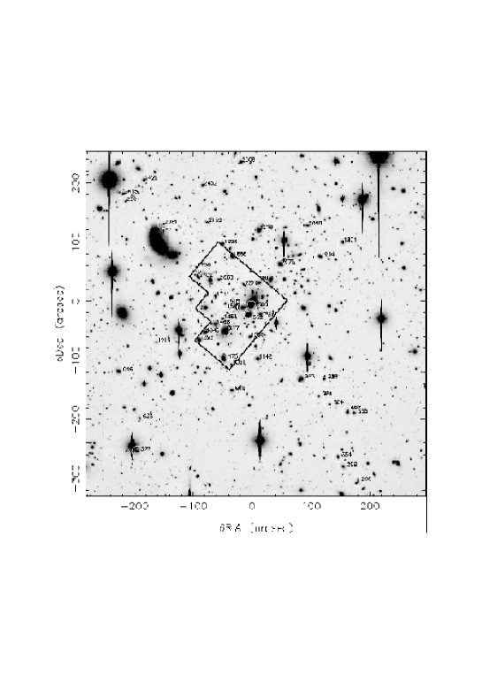
Figure 9: $I$-band image of the cluster A 2218 taken with the 5.1-m Hale telescope. The labels correspond to the galaxy numbers of Table 4. North is up and East to the left. Coordinates are distance from the central galaxy in arcseconds. The HST field-of-view is indicated as well.

Place Fig. mosaic_p200.jpg here.

Place Fig. mosaic_p200b.jpg here.

Figure 10: $20^{\prime\prime}\times 20^{\prime\prime}$ sections from the Hale $I$-band images of each of the spectroscopically confirmed cluster members in our sample. These panels have North top and East left and the contours are in 0.5 mag increments with the faintest contour being $\mu_{I}=21.5$ mag arcsec^-2. The labels give the galaxy ID as listed in Table 4 and where available the morphology from the HST image.

Table 4:

ID	R.A.	Dec.	$I_{\mathrm{tot}}$	$U_{\mathrm{ap}}$	$B_{\mathrm{ap}}$	$V_{\mathrm{ap}}$	$I_{\mathrm{ap}}$
	(J2000)
208	16 35 19.89	$+$66 07 41.5	17.224	21.431$\pm$0.053	21.031$\pm$0.004	19.611$\pm$0.003	17.832$\pm$0.002
299	16 35 23.91	$+$66 08 05.9	17.128	20.715$\pm$0.016	20.362$\pm$0.003	19.097$\pm$0.003	17.538$\pm$0.002
354	16 35 25.42	$+$66 08 22.3	17.751	21.706$\pm$0.012	21.208$\pm$0.004	19.789$\pm$0.003	18.151$\pm$0.002
377	16 36 21.37	$+$66 08 32.6	17.311	21.359$\pm$0.007	20.969$\pm$0.008	19.532$\pm$0.005	17.801$\pm$0.004
626	16 36 20.64	$+$66 09 28.3	17.509	21.426$\pm$0.009	21.082$\pm$0.004	19.541$\pm$0.003	17.914$\pm$0.002
665	16 35 20.86	$+$66 09 36.0	17.131	20.749$\pm$0.005	20.514$\pm$0.003	19.193$\pm$0.003	17.611$\pm$0.002
697	16 35 22.66	$+$66 09 37.7	17.142	21.079$\pm$0.007	20.725$\pm$0.004	19.230$\pm$0.003	17.571$\pm$0.002
704	16 35 27.58	$+$66 09 50.5	18.320	21.679$\pm$0.008	21.512$\pm$0.004	20.162$\pm$0.003	18.571$\pm$0.002
786	16 35 30.67	$+$66 10 04.5	17.950	21.618$\pm$0.007	21.295$\pm$0.004	19.795$\pm$0.002	18.154$\pm$0.001
849	16 35 54.85	$+$66 10 14.5	17.203	21.230$\pm$0.007	20.878$\pm$0.004	19.326$\pm$0.003	17.703$\pm$0.002
926	16 35 29.09	$+$66 10 33.8	17.900	21.912$\pm$0.008	21.510$\pm$0.005	19.997$\pm$0.004	18.374$\pm$0.002
983	16 35 35.53	$+$66 10 34.0	16.210	20.809$\pm$0.006	20.416$\pm$0.004	18.826$\pm$0.004	17.187$\pm$0.003
1046	16 36 26.42	$+$66 10 47.3	16.824	20.961$\pm$0.006	20.642$\pm$0.003	19.086$\pm$0.003	17.472$\pm$0.002
1051	16 35 54.96	$+$66 10 58.6	18.235	22.207$\pm$0.013	21.796$\pm$0.006	20.238$\pm$0.004	18.601$\pm$0.003
1142	16 35 47.59	$+$66 11 07.8	16.618	20.634$\pm$0.005	20.298$\pm$0.003	18.773$\pm$0.003	17.206$\pm$0.002
1175	16 35 57.14	$+$66 11 08.1	16.132	20.633$\pm$0.007	20.270$\pm$0.005	18.663$\pm$0.005	17.079$\pm$0.004
1213	16 36 15.88	$+$66 11 35.9	17.785	21.452$\pm$0.007	21.144$\pm$0.004	19.608$\pm$0.002	18.035$\pm$0.001
1256	16 35 49.79	$+$66 11 44.5	17.683	21.827$\pm$0.011	21.489$\pm$0.006	19.982$\pm$0.005	18.409$\pm$0.003
1293	16 36 03.95	$+$66 11 40.0	16.711	21.038$\pm$0.007	20.642$\pm$0.004	18.972$\pm$0.003	17.333$\pm$0.002
1343	16 36 02.25	$+$66 11 52.5	16.775	20.974$\pm$0.006	20.571$\pm$0.004	18.914$\pm$0.003	17.278$\pm$0.002
1437	16 35 56.74	$+$66 11 55.2	15.403	21.200$\pm$0.011	20.776$\pm$0.009	19.097$\pm$0.009	17.461$\pm$0.008
1454	16 35 57.35	$+$66 12 15.3	17.768	21.515$\pm$0.007	21.183$\pm$0.004	19.605$\pm$0.003	17.988$\pm$0.002
1466	16 35 59.34	$+$66 12 06.3	16.415	21.237$\pm$0.008	20.826$\pm$0.005	19.224$\pm$0.004	17.598$\pm$0.003
1516	16 35 46.76	$+$66 12 22.5	17.454	21.452$\pm$0.008	21.131$\pm$0.006	19.597$\pm$0.005	18.007$\pm$0.004
1552	16 35 49.92	$+$66 12 23.4	16.514	20.995$\pm$0.008	20.578$\pm$0.006	18.955$\pm$0.005	17.312$\pm$0.005
1580	16 35 49.38	$+$66 12 35.9	17.097	21.081$\pm$0.012	20.751$\pm$0.010	19.206$\pm$0.010	17.640$\pm$0.009
1605	16 35 56.65	$+$66 12 40.9	17.992	21.406$\pm$0.007	21.154$\pm$0.004	19.778$\pm$0.003	18.315$\pm$0.002
1662	16 35 51.78	$+$66 12 34.0	16.634	20.732$\pm$0.006	20.343$\pm$0.004	18.762$\pm$0.004	17.163$\pm$0.003
1711	16 35 59.31	$+$66 12 53.2	17.293	21.269$\pm$0.007	20.919$\pm$0.004	19.357$\pm$0.003	17.760$\pm$0.002
1831	16 35 23.68	$+$66 14 23.1	17.235	21.223$\pm$0.006	20.862$\pm$0.003	19.331$\pm$0.002	17.684$\pm$0.002
1888	16 35 54.60	$+$66 14 00.2	16.561	20.882$\pm$0.007	20.585$\pm$0.006	19.044$\pm$0.005	17.488$\pm$0.004
1914	16 35 30.09	$+$66 13 59.6	17.044	21.097$\pm$0.007	20.807$\pm$0.004	19.329$\pm$0.004	17.699$\pm$0.003
1928	16 35 57.21	$+$66 14 21.4	17.337	21.221$\pm$0.008	20.910$\pm$0.004	19.336$\pm$0.003	17.709$\pm$0.002
1976	16 35 47.23	$+$66 14 44.4	16.089	20.454$\pm$0.005	20.105$\pm$0.003	18.517$\pm$0.003	16.930$\pm$0.002
2061	16 36 13.77	$+$66 14 54.7	18.165	21.945$\pm$0.014	21.688$\pm$0.009	20.258$\pm$0.009	18.664$\pm$0.004
2076	16 35 41.15	$+$66 13 46.8	16.274	20.694$\pm$0.006	20.353$\pm$0.004	18.740$\pm$0.004	17.123$\pm$0.003
2090	16 35 33.51	$+$66 14 51.6	17.462	21.232$\pm$0.006	20.949$\pm$0.004	19.480$\pm$0.003	17.898$\pm$0.002
2139	16 36 01.55	$+$66 14 57.4	17.802	21.467$\pm$0.008	21.268$\pm$0.004	19.860$\pm$0.003	18.257$\pm$0.002
2270	16 35 51.39	$+$66 13 11.9	17.428	21.512$\pm$0.009	21.107$\pm$0.004	19.531$\pm$0.003	17.925$\pm$0.002
2304	16 36 24.41	$+$66 15 32.9	18.331	21.936$\pm$0.009	21.550$\pm$0.004	20.138$\pm$0.003	18.567$\pm$0.002
2452	16 36 02.77	$+$66 16 00.1	17.387	21.318$\pm$0.008	21.083$\pm$0.004	19.604$\pm$0.003	17.936$\pm$0.002
2508	16 35 52.09	$+$66 16 39.0	17.465	21.338$\pm$0.010	21.060$\pm$0.006	19.565$\pm$0.006	17.939$\pm$0.004
2604	16 35 47.16	$+$66 13 15.8	17.106	21.138$\pm$0.006	20.808$\pm$0.004	19.217$\pm$0.003	17.605$\pm$0.002
2615	16 36 24.96	$+$66 15 45.8	17.460	21.404$\pm$0.008	21.053$\pm$0.004	19.598$\pm$0.003	18.001$\pm$0.002
2660	16 35 58.27	$+$66 13 21.2	17.895	21.824$\pm$0.010	21.549$\pm$0.004	20.000$\pm$0.003	18.402$\pm$0.002
2702	16 36 04.16	$+$66 13 25.0	16.923	20.863$\pm$0.006	20.516$\pm$0.004	18.882$\pm$0.003	17.285$\pm$0.002
2738	16 36 04.76	$+$66 13 42.2	18.271	21.939$\pm$0.010	21.663$\pm$0.005	20.107$\pm$0.003	18.485$\pm$0.002

The galaxy ID can be found in the finding chart (Fig. 9), $I_{\mathrm{tot}}$ is the total magnitude derived from the Hale images (SExtractor’s best_mag), $U_{\mathrm{ap}}$, $B_{\mathrm{ap}}$, $V_{\mathrm{ap}}$, and $I_{\mathrm{ap}}$ are magnitudes within a circular aperture of 4.0″ diameter measured in the seeing-convolved images. None of the given magnitudes are corrected for extinction.

Appendix B Kinematic and structural parameters for the HST subsample

blablabla

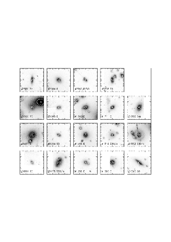
Figure 11: Images of the 19 galaxies in our spectroscopic sample which fall within the HST/WFPC2 field of A 2218. Each panel is $20^{\prime\prime}$ square and is labelled with the galaxy ID and visual morphology from Table 5.

Table 5:

ID	$\log(\sigma_{a})$	$R_{702}$	$\log\langle I_{e}\rangle$	$r_{e}$	$\log(R_{e})$	$r_{e,b}$	$h$	$d/b$	type
0	2.50	14.81	1.43	18.347	1.85	30.00	2.75	0.27	cD
1051	2.04	18.83	2.85	0.562	0.33	0.56	…	0.00	S0
1175	2.28	16.71	2.60	1.976	0.88	1.98	…	0.00	SB0/a
1256	2.18	18.29	2.26	1.421	0.74	1.12	1.75	0.22	E
1293	2.38	17.42	2.92	0.997	0.58	0.75	0.82	0.49	E
1343	2.38	17.26	3.01	0.968	0.57	1.70	0.20	0.33	S0
1437	2.40	15.68	1.69	9.214	1.55	6.65	8.22	0.48	E
1454	2.34	18.03	2.90	0.771	0.47	0.48	3.23	0.27	S0
1466	2.30	17.23	2.37	2.055	0.90	2.05	…	0.00	E
1516	2.07	18.15	2.88	0.745	0.46	0.75	…	0.00	SB0/a
1552	2.23	16.89	2.45	2.198	0.93	2.56	0.10	0.08	SB0/a
1580	2.21	17.91	2.98	0.732	0.45	0.73	…	0.00	S0
1605	2.13	18.51	2.70	0.761	0.47	0.59	0.63	0.43	E
1662	2.56	17.08	2.90	1.186	0.66	1.60	0.11	0.16	E
1711	2.31	17.95	2.90	0.794	0.48	0.59	0.95	0.29	E
1888	2.19	17.44	2.62	1.380	0.72	0.38	1.15	2.02	Sab
2270	2.23	17.96	2.63	1.082	0.62	1.08	…	0.00	Sa
2604	2.27	17.67	2.88	0.931	0.55	0.93	…	0.00	E
2660	2.08	18.68	2.48	0.926	0.55	0.93	…	0.00	E/S0
2702	2.35	17.49	3.10	0.782	0.48	0.78	0.47	0.21	S0

The galaxy ID can be found in the finding chart (Fig. 9) and coordinates are given in Table 4, $\log(\sigma_{a})$ is the logarithm of the aperture corrected velocity dispersion (the value for the cD galaxy # 0 was taken from JFHD99), $R_{702}$ is the extinction-corrected, Vega-based total magnitude in the WFPC2 F702W filter, $\log\langle I_{e}\rangle$ is the mean surface brightness within the effective radius $r_{e}$ (in arcsec) in the $I$ band according to Equation 8, $\log(R_{e})$ is the logarithm of the effective radius (in kpc), $r_{e,b}$ is the effective radius of the bulge, $h$ is the scale-length of the disk (both in arcsec) and $d/b$ is the luminosity weighted disk-to-bulge ratio (see Section 4.1.3 for the derivation). The galaxy types were obtained visually by Prof. Couch. Thumbnail images are shown in Fig. 11.

Appendix C Spectroscopic data

Table 6:

ID	$\sigma$	$v$	H$\beta$	Mgb	S/N	disk
208	181.1$\pm$5.6	46505$\pm$18	1.62$\pm$0.14	4.17$\pm$0.15	50	d
299	163.3$\pm$5.0	45708$\pm$15	2.64$\pm$0.11	2.72$\pm$0.12	133
354	105.5$\pm$7.2	48949$\pm$28	2.49$\pm$0.15	3.30$\pm$0.16	65
377	247.0$\pm$4.9	48505$\pm$17	2.03$\pm$0.18	4.10$\pm$0.20	137
626	128.1$\pm$5.3	46573$\pm$19	1.97$\pm$0.21	3.98$\pm$0.24	84
665	126.1$\pm$7.2	46577$\pm$22	2.09$\pm$0.13	2.54$\pm$0.14	99
697	189.5$\pm$8.6	49622$\pm$12	2.05$\pm$0.11	3.84$\pm$0.13	76	d
704	105.6$\pm$8.7	47276$\pm$17	2.49$\pm$0.24	3.27$\pm$0.26	70
786	137.1$\pm$4.9	50537$\pm$10	1.77$\pm$0.16	3.64$\pm$0.17	93
849	204.6$\pm$8.6	45484$\pm$18	1.37$\pm$0.11	4.34$\pm$0.13	82
926	132.6$\pm$4.8	49293$\pm$14	2.34$\pm$0.22	3.98$\pm$0.23	68
983	198.3$\pm$5.5	48917$\pm$17	1.47$\pm$0.09	4.40$\pm$0.10	132
1046	247.1$\pm$4.8	46372$\pm$15	1.80$\pm$0.13	4.33$\pm$0.14	41
1051	105.6$\pm$4.9	48272$\pm$23	1.72$\pm$0.24	4.23$\pm$0.26	53	d
1142	194.2$\pm$5.3	45491$\pm$15	1.93$\pm$0.09	3.88$\pm$0.10	113
1175	182.8$\pm$5.2	48256$\pm$14	2.03$\pm$0.08	3.94$\pm$0.09	140	d
1213	150.1$\pm$4.6	48067$\pm$22	1.87$\pm$0.18	3.99$\pm$0.21	75
1256	145.7$\pm$5.1	49638$\pm$ 1	1.91$\pm$0.22	3.97$\pm$0.23	72
1293	229.1$\pm$4.8	47896$\pm$17	1.60$\pm$0.11	4.78$\pm$0.13	109
1343	230.6$\pm$4.9	50027$\pm$15	1.87$\pm$0.11	4.67$\pm$0.12	110	d
1437	237.3$\pm$4.5	48495$\pm$15	1.76$\pm$0.10	4.74$\pm$0.11	127
1454	210.0$\pm$5.5	49624$\pm$ 9	1.77$\pm$0.19	4.40$\pm$0.21	103	d
1466	189.9$\pm$5.1	49405$\pm$12	1.88$\pm$0.14	4.17$\pm$0.15	107
1516	111.8$\pm$7.0	44919$\pm$13	2.15$\pm$0.15	3.40$\pm$0.16	78	d
1552	161.4$\pm$5.4	48842$\pm$19	2.05$\pm$0.11	3.78$\pm$0.13	43	d
1580	155.5$\pm$4.7	47850$\pm$14	2.05$\pm$0.13	3.81$\pm$0.14	122	d
1605	128.3$\pm$4.7	47050$\pm$17	2.67$\pm$0.18	3.57$\pm$0.19	86
1662	348.5$\pm$5.6	44948$\pm$28	1.80$\pm$0.09	5.35$\pm$0.11	150
1711	194.5$\pm$5.4	47619$\pm$20	1.81$\pm$0.15	4.60$\pm$0.17	89
1831	182.2$\pm$5.5	47833$\pm$14	1.84$\pm$0.15	4.40$\pm$0.17	80
1888	147.1$\pm$5.3	47906$\pm$ 4	2.50$\pm$0.11	3.29$\pm$0.12	86	d
1914	140.8$\pm$5.1	47556$\pm$15	1.65$\pm$0.16	4.20$\pm$0.18	87
1928	207.0$\pm$4.6	48684$\pm$14	2.00$\pm$0.12	3.88$\pm$0.13	137
1976	266.2$\pm$5.0	46339$\pm$17	1.56$\pm$0.08	4.48$\pm$0.09	145
2061	131.5$\pm$8.2	49002$\pm$ 8	1.65$\pm$0.24	3.68$\pm$0.26	73
2076	209.1$\pm$5.2	49399$\pm$15	1.63$\pm$0.09	4.16$\pm$0.10	138
2090	134.4$\pm$5.3	49211$\pm$15	2.13$\pm$0.19	3.81$\pm$0.21	86	d
2139	114.5$\pm$6.5	48905$\pm$ 2	1.96$\pm$0.18	3.14$\pm$0.19	59	d
2270	160.6$\pm$5.2	46078$\pm$12	1.39$\pm$0.20	4.26$\pm$0.22	79	d
2304	101.6$\pm$4.7	46568$\pm$17	3.53$\pm$0.23	3.48$\pm$0.25	60
2429	163.3$\pm$4.9	46235$\pm$12	2.12$\pm$0.20	3.80$\pm$0.22	46
2452	127.3$\pm$4.8	46286$\pm$16	1.66$\pm$0.17	3.92$\pm$0.19	68	d
2508	128.0$\pm$5.3	47114$\pm$17	1.47$\pm$0.14	3.87$\pm$0.15	102
2604	179.3$\pm$9.9	49390$\pm$17	1.97$\pm$0.12	4.22$\pm$0.13	86
2615	155.0$\pm$5.2	49558$\pm$12	2.11$\pm$0.16	3.32$\pm$0.17	83
2660	114.8$\pm$4.5	48561$\pm$15	1.42$\pm$0.23	4.18$\pm$0.25	63	d
2702	212.3$\pm$5.5	47747$\pm$14	1.89$\pm$0.09	4.39$\pm$0.10	156	d
2738	173.7$\pm$5.5	47723$\pm$14	1.86$\pm$0.21	4.18$\pm$0.23	76

The galaxy ID can be found in the finding chart (Fig. 9) and coordinates are given in Table 4, $\sigma$ is the velocity dispersion measured in km s^-1 (not aperture corrected) and its error, $v$ the radial velocity and its error. The line indices are measured in the flux-calibrated spectra and given in Å. The signal-to-noise ratio is given in the last but one column, while the last column indicates whether the galaxy has a strong disk (d).

Figure 12: A 2218 example spectra shown in the observed frame. Spectra were degraded to the Lick resolution for measurement of the indices (for identification, see Fig. 2). The left panels show spectra with decreasing S/N ($\sigma$) from top to bottom, whereas the right panels show ‘peculiar’ galaxies (1662: high $\sigma$, 2270: low H$\beta$, 299: low Mg_b) and the skylines.

Appendix D Bootstrap bisector fits

Table 7:

Relation	Local	A 2218: Full	E	S0	In	Out
(1) $\log\sigma$–Mgb	3.80$\pm$0.35	3.97$\pm$0.49	4.18$\pm$0.67	3.15/1.01	3.61$\pm$0.57	3.96$\pm$0.52
	4.40$\pm$0.06	4.33$\pm$0.06	4.28$\pm$0.08	4.40$\pm$0.09	4.39$\pm$0.09	4.27$\pm$0.09
		$-$0.07	$-$0.12	0	$-$0.01	$-$0.13
	-4.10	$-$4.55	$-$5.08	$-$2.66	$-$3.70	$-$4.59
	72	48	31	16	24	24
(1a) $\log\sigma$–Mgb		3.54$\pm$0.31	3.37$\pm$0.39
		4.39$\pm$0.04	4.37$\pm$0.05
		$-$0.01	$-$0.03
		$-$3.53	$-$3.18
		46	29
(2) $\log\sigma$–$r_{\rm abs}$	$-$6.82$\pm$0.89	$-$5.10$\pm$0.69	$-$5.44$\pm$0.35	$-$4.32$\pm$0.99	$-$5.46$\pm$0.90	$-$4.30$\pm$0.75
	$-$21.49$\pm$0.06	$-$21.80$\pm$0.07	$-$21.78$\pm$0.06	$-$21.95$\pm$0.13	$-$21.81$\pm$0.14	$-$21.77$\pm$0.08
		$-$0.31	$-$0.29	$-$0.45	$-$0.32	$-$0.28
	$-$6.23	$-$10.38	$-$9.59	$-$12.28	$-$9.60	$-$12.14
	75	48	31	16	24	24
(3) $\log(R_{e})$–FP	1.05$\pm$0.05	1.13$\pm$0.08	1.08$\pm$0.06	1.05$\pm$0.18
	0.58$\pm$0.01	0.52$\pm$0.02	0.60$\pm$0.03	0.49$\pm$0.04
		$-$0.06	0.02	$-$0.11
	0.03	$-$0.07	0.03	$-$0.06
	88	20	9	11
(4) $\log\sigma$–$\log(M/L)$	1.27$\pm$0.13	1.61$\pm$0.17	1.52$\pm$0.42	1.18$\pm$0.31
	0.60$\pm$0.01	0.52$\pm$0.02	0.58$\pm$0.05	0.47$\pm$0.04
		$-$0.08	$-$0.02	$-$0.13
	$-$2.29	$-$3.16	$-$2.88	$-$2.23
	102	20	9	11

1. row: slope$\pm 1\sigma$

2. row: $y(\langle x\rangle)$ i.e. ordinate value at median value of abscissa

3. row: $\Delta$(A 2218–local)

4. row: zeropoint

5. row: number of galaxies

Local sample: (1) SMAC (full sample), (2) Jøergensen reduced to value range of A 2218: $\log(\sigma)>2.0$, $r_{\rm abs}<-20.7$, (3) Jøergensen reduced to value range of A 2218: $\log(R_{e})>0.26$,FP$>0.20$, (4) Jøergensen reduced to value range of A 2218: $\log(\sigma)>2.0$

Distant sample: A 2218 full sample; E: only ellipticals; S0: only lenticulars; In: only core sample; Out: only outer region sample; (1a) full sample without #299 and #665

References

- [\citefmtAbadi et al.1999] Abadi, M.G., Moore, B., Bower, R.G., 1999, MNRAS, 308, 947.
- [\citefmtAbraham et al.1996] Abraham, R., et al., 1996, ApJ, 471, 694.
- [\citefmtAllington-Smith et al.1994] Allington-Smith, J.R, et al., 1994, PASP, 106, 983.
- [\citefmtAaronson1978] Aaronson, M., 1978, ApJ, 221, L103
- [\citefmtBalogh et al.1999] Balogh, M.L., Morris, S.L., Yee, H.K.C., Carlberg, R.G., Ellingson, E., 1999 ApJ, 527, 54.
- [\citefmtBarger et al.1998] Barger, A.J., Aragón-Salamanca, A., Smail, I., Ellis, R.S., Couch, W.J., Dressler, A., Oemler, A., Poggianti, B.M., Sharples, R.M., 1998, ApJ, 501, 522.
- [\citefmtBarrientos et al.1996] Barrientos, L.F., Schade, D., López-Cruz, O., 1996, ApJ, 460, L89.
- [\citefmtBender1990] Bender, R., 1990, A&A, 229, 441.
- [\citefmtBender et al.1992] Bender, R., Burstein, D., Faber, S.M., 1992, ApJ, 399, 462.
- [\citefmtBender et al.1993] Bender, R., Burstein, D., Faber, S.M., 1993, ApJ, 411, 153.
- [\citefmtBender & Möllenhoff1987] Bender, R. Möllenhoff, C., 1987, A&A, 177, 71.
- [\citefmtBender et al.1998] Bender, R., Saglia, R.P., Ziegler, B., Belloni, P., Bruzual, G., Greggio, L., Hopp, U., 1998, ApJ, 493, 529.
- [\citefmtBender et al.1996] Bender, R., Ziegler, B., Bruzual, G., 1996, ApJ, 463, L51.
- [\citefmtBertin & Arnouts1996] Bertin, E., Arnouts, S., 1996, A&AS, 117, 393.
- [\citefmtBruzual & Charlot1993] Bruzual, G.A., Charlot, S., 1993, ApJ, 405, 538.
- [\citefmtButcher & Oemler1984] Butcher, H., Oemler A., 1984, ApJ, 285, 426
- [\citefmtCasuso et al.1996] Casuso, E., Vazdekis, A., Peletier, R.F., Beckman, J., 1996, ApJ, 458, 533.
- [\citefmtColless et al.1999] Colless, M., Burstein, D., Davies, R.L., McMahan, R.K., Saglia, R.P., Wegner, G., 1999, MNRAS, 303, 813.
- [\citefmtCouch et al.1998] Couch, W.J., Barger, A.J., Smail, I., Ellis, R.S., Sharples, R.M., 1998, ApJ, 497, 188.
- [\citefmtCouch et al.1994] Couch, W.J., Ellis, R.S., Sharples, R.M., Smail, I., 1994, ApJ, 430, 121.
- [\citefmtDjorgovski & Davis1987] Djorgovski, S., Davis, M., 1987, ApJ, 313, 59.
- [\citefmtDressler et al.1987] Dressler, A., Lynden-Bell, D., Burstein, D., Davies, R.L., Faber, S.M., Terlevich, R.J., Wegner, G., 1987, ApJ, 313, 42.
- [\citefmtDressler et al.1997] Dressler, A., Oemler Jr., A., Couch, W.J., Smail, I., Ellis, R.S., Barger, A., Butcher, H., Poggianti, B.M., Sharples, R.M., 1997, ApJ, 490, 577.
- [\citefmtEllis et al.1997] Ellis, R.S., Smail, I., Dressler, A., Couch, W.J., Oemler, A., Butcher, H., Sharples, R.M., 1997, ApJ, 483, 582
- [\citefmtFaber et al.1985] Faber, S.M., Friel, E.D., Burstein, D., Gaskell, C.M., 1985, ApJS, 57, 711.
- [\citefmtFaber & Jackson1976] Faber, S.M., Jackson, R.E., 1976, ApJ, 204, 668.
- [\citefmtFasano et al.1998] Fasano, G., Cristiani, S., Arnouts, S., Filippi, M., 1998, AJ, 115, 1400.
- [\citefmtHill et al.1998] Hill, R.J. et al., 1998, ApJ, 496, 648.
- [\citefmtHoltzman et al.1995] Holtzman, J.A., Burrows, C.J., Casertano, S., Hester, J.J., Trauger, J.T., Watson, A.M., Worthey, G., 1995, PASP, 107, 1065.
- [\citefmtHorne1986] Horne, K., 1986, PASP, 98, 609.
- [\citefmtJones & Worthey1995] Jones, L.A., Worthey, G., 1995, ApJL, 446, L31.
- [\citefmtJones, Smail & Couch2000] Jones, L.A., Smail, I., Couch, W.J., 2000, ApJ, 528, 118.
- [\citefmtJørgensen1999] Jørgensen, I., 1999, MNRAS, 306, 607.
- [\citefmtJørgensen et al.1999] Jørgensen, I., Franx, M., Hjorth, J., van Dokkum, P.G., 1999, MNRAS, 308, 833 (JFHD).
- [\citefmtJørgensen et al. 1995a] Jørgensen, I., Franx, M., Kjærgaard, P., 1995a, MNRAS, 273, 1097.
- [\citefmtJørgensen et al. 1995b] Jørgensen, I., Franx, M., Kjærgaard, P., 1995b, MNRAS, 276, 1341.
- [\citefmtJørgensen et al.1996] Jørgensen, I., Franx, M., Kjærgaard, P., 1996, MNRAS, 280, 167.
- [\citefmtKelson et al. 2000b] Kelson, D.D., Illingworth, G.D., van Dokkum, P.G., Franx, M., 2000b, ApJ, 531, 184.
- [\citefmtKelson et al.1997] Kelson, D.D., van Dokkum, P.G., Franx, M., Illingworth, G.D., Fabricant, D., 1997, ApJ, 478, L13.
- [\citefmtKent1985] Kent, S.M., 1985, PASP, 97, 165.
- [\citefmtKneib et al.1996] Kneib, J.-P., Ellis, R.S., Smail, I., Couch, W.J, Sharples, R.M., 1996, ApJ, 471, 643.
- [\citefmtKodama & Bower 2000] Kodama, T., Bower, R.G., 2000, MNRAS. in press.
- [\citefmtKodama & Smail2000] Kodama, T., Smail, I., 2001, ApJL, submitted.
- [\citefmtKormendy 1977] Kormendy, J., 1977, ApJ, 218, 333.
- [\citefmtKrist & Hook1997] Krist, R., Hook, R., 1997, The Tiny Tim User’s Manual, STScI, Baltimore
- [\citefmtKuntschner2000] Kuntschner, H., 2000, MNRAS, 315, 184.
- [\citefmtKuntschner & Davies1998] Kuntschner, H., Davies, R.L., 1998, MNRAS, 295, L29.
- [\citefmtKuntschner et al.2000] Kuntschner, H., Lucey, J.R., Smith, R.J., Hudson, M.J., Davies, R.L., 2000, MNRAS. submitted.
- [\citefmtLandolt1992] Landolt, A.U., 1992, AJ, 104, 340.
- [\citefmtLarson et al.1980] Larson, R.B., Tinsley, B.M., Caldwell, C.N., 1980, ApJ, 237, 692.
- [\citefmtLe Borgne et al.1992] Le Borgne, J.F., Pello, R., Sanahuja, B., 1992, A&AS, 95, 87.
- [\citefmtMehlert et al.2000] Mehlert, D., Saglia, R.P., Bender, R., Wegner, G., 2000, A&AS, 141, 449.
- [\citefmtMoles et al.1998] Moles, M., Campos, A., Kjærgaard, P., Fasano, G., Bettoni, D., 1998, ApJ, 495, L31.
- [\citefmtPahre et al.1996] Pahre, M.A., Djorgovski, S., deCarvalho, R.R., 1996, ApJ, 456, L79.
- [\citefmtPimbblet et al.2001] Pimbblet, K.A., Kodama, T., Smail, I., Edge, A.C., Couch, W.J., Zabludoff, A.I., O’Hely, E., 2001, in prep.
- [\citefmtPoggianti et al.1999] Poggianti, B.M., Smail, I., Dressler, A., Couch, W.J., Barger, A., Butcher, H., Ellis, R.S., Oemler Jr., A., 1999, ApJ, 518, 576.
- [\citefmtQuilis et al.2000] Quilis, V., Moore, B., Bower, R., 2000, Science, 288, 1617.
- [\citefmtSaglia et al.1993] Saglia, R.P., Bender, R., Dressler, A., 1993, A&A, 279, 75.
- [\citefmtSaglia et al.1997a] Saglia, R.P., Bertschinger, E., Baggley, G., Burstein, D., Colless, M., Davies, R.L., McMahan Jr., R.K., Wegner, G., 1997a, ApJS, 109, 79.
- [\citefmtSaglia et al.1997b] Saglia, R.P., Burstein, D., Baggley, G., Davies, R.L., Bertschinger, E., Colless, M., McMahan Jr., R.K., Wegner, G., 1997b, MNRAS, 292, 499.
- [\citefmtSchade et al.1997] Schade, D., Barrientos, L.F., Lopéz-Cruz, O., 1997, ApJ, 477, L17.
- [\citefmtSchade et al.1996] Schade, D., Carlberg, R.G., Yee, H. K.C., Lopéz–Cruz, O., Ellingson, E., 1996, ApJ, 464, L63.
- [\citefmtSchaifers et al.1981] Schaifers, K., Vogt, H.H. (eds.), 1981, Landolt–Börnstein series, Vol. VI/2a, Springer.
- [\citefmtSchlegel et al.1998] Schlegel, D.J., Finkbeiner, D.P., Davis, M., 1998, ApJ, 500, 525.
- [\citefmtSmail et al.1998] Smail, I., Edge, A.C., Ellis, R.S., Blandford, R.D., 1998, MNRAS, 293, 124.
- [\citefmtSmail et al.2001] Smail, I., Kuntschner, H., Kodama, T., Smith, G.P., Packham, C., Fruchter, A.S., Hook, R.N., 2001, MNRAS, in press.
- [\citefmtThomas et al.1999] Thomas, D., Greggio, L., Bender, R., 1999, MNRAS, 302, 537.
- [\citefmtTrager1997] Trager, S. C., 1997, PhD Thesis, University of California at Santa Cruz.
- [\citefmtvan Dokkum & Franx1996] van Dokkum, P.G., Franx, M., 1996, MNRAS, 281, 985.
- [\citefmtvan Dokkum et al.1998a] van Dokkum, P.G., Franx, M., Kelson, D.D., Illingworth, G.D., Fisher, D., Fabricant, D., 1998a, ApJ, 500, 714.
- [\citefmtvan Dokkum et al.1998b] van Dokkum, P.G., Franx, M., Kelson, D.D., Illingworth, G.D., 1998b, ApJ, 504, L17.
- [\citefmtVazdekis & Arimoto1999] Vazdekis, A., Arimoto, N., 1999, ApJ, 458, 533.
- [\citefmtWorthey1994] Worthey, G., 1994, ApJS, 95, 107.
- [\citefmtWorthey & Ottaviani1997] Worthey, G., Ottaviani, D.L., 1997, ApJS, 111, 377.
- [\citefmtZiegler et al. 1999] Ziegler, B., Saglia, R.P., Bender, R., Belloni, P., Greggio, L., Seitz, S., 1999, A&A, 346, 13.
- [\citefmtZiegler & Bender1997] Ziegler, B.L., Bender, R., 1997, MNRAS, 291, 527.