Quiescent and flare analysis for the chromospherically active star Gl 355 (LQ Hya)

We discuss ROSAT and ASCA observations of the young active star Gl 355. During the ROSAT observation a strong flare was detected with a peak flux more than an order of magnitude larger than the quiescent level. Spectral analysis of the data allows us to study the temperature and emission measure distribution, and the coronal metal abundance, for the quiescent phase and, in the case of ROSAT, also during the evolution of the flare. The global coronal metallicity $Z/Z_{\odot}\sim 0.1$ derived from both ROSAT and ASCA data is much lower than solar and presumably also much lower than the photospheric abundance expected for this very young star. The temperature structure of the quiescent corona was about the same during the various observations, with a cooler component at $T_{1}\sim 7$ MK and a hotter component (to which only ASCA was sensitive) at $T_{2}\sim 20$ MK. During the flare, the low temperature component remained approximately constant and equal to the quiescent value, while the high-temperature component was the only one that varied. We have modeled the flare with the hydrodynamic-decay sustained-heating approach of Reale at al. (1997) and we have derived a loop semi–length of the order of $\sim 1.5$ stellar radii, i.e. much larger than the dimensions of flares on the Sun, but comparable with the typical dimensions inferred for other stellar flares. We have compared the derived loop size with that estimated with a simpler (but physically inconsistent) approach, finding that for this, as well for several other stellar flares, the two methods give comparable loop sizes. Possible causes and consequences of this result are discussed.

1 Introduction

It has been known for a long time that a subset of late K and M dwarf stars in the solar neighborhood are characterized by the occurrence of flares at optical, UV, X–ray and radio wavelengths. Moreover, all types of late–type stars show flaring activity in their soft X–ray emission (see for instance Schmitt Sch94 (1994)). Flares on the Sun and on dKe–dMe stars are usually believed to be basically similar in their origin and development, in spite of the fact that stellar flares are normally $2\div 4$ orders of magnitude more energetic than the largest solar flares. Magnetic coupling between the components in a binary system or between a young star and an accretion disk has been invoked to explain the energy budget for some giant flares (Graffagnino et al. GWS95 (1995), Grosso et al. GMF97 (1997), van den Oord v88 (1988)).

One of the fundamental problems in the study of stellar flares is the determination of the geometry and size of the flaring coronal plasma. Indeed stellar coronae, as shown by spatially resolved observations of the solar corona, are far from being spatially homogeneous. The lack of spatial information is a strong limitation for the study of stellar coronae: low–resolution coronal X–ray spectra are insensitive to the plasma density and do not allow distinguishing between an extended low-pressure emitting region and a compact high pressure one. Indeed, spatial information about the size of a flare could help to discriminate between different theoretical scenarios. For instance, it is accepted that the decay time of a flare X–ray light curve is related to the length of the flaring loop. This property is often used to derive the spatial size of unresolved flares, assuming that there is no heating in the decay (e.g. Haisch Hai83 (1983), White et al. WCP86 (1986), van den Oord & Mewe vM89 (1989), Pallavicini et al. PTS90 (1990), Pallavicini P95b (1995)). However, if a significant amount of heating is present during the flare decay, the derived loop lengths can be in error.

Thus far, the main tools to study the spatial distribution of stellar coronal plasmas have been eclipse monitorings and the study of flares. However, as discussed by Schmitt (S98 (1998)) convincing examples of rotationally modulated X–ray emission are rare and eclipse observations often do not produce unambiguous results (see for instance White et al. WSP90 (1990), Culhane et al. CWSP90 (1990), Tagliaferri et al. TWD91 (1991), Schmitt & Kürster SK93 (1993), Ottmann et al. OSK93 (1993), Kürster & Dennerl KD93 (1993), White et al. 1994a , Ottmann O94 (1994), Antunes et al. ANW94 (1994), Huenemoerder H98 (1998), Tagliaferri et al. TCCP99 (1999), Rodonò et al. RPL99 (1999)). Recently the observation of the total eclipse of a large flare on Algol (Schmitt & Favata SF99 (1999)) has for the first time yielded a strong geometrical constraint on the size of a flaring structure. However, apart from this unique case, most estimates of stellar flare sizes have relied on modeling approaches (e.g. Ortolani et al. OPMRW98 (1998), Favata and Schmitt FS99 (1999), Maggio et al. MPRT00 (2000)).

Several reviews of the X–ray properties of flare stars based on observations performed by different satellites and/or detectors have appeared in the literature: from Einstein data (Haisch Hai83 (1983), Ambruster et al. ASG89 (1989)); EXOSAT data (Pallavicini et al. PTS90 (1990)); and ROSAT data (Schmitt Sch94 (1994)). A review about the status of solar and stellar flare research has been published by Haisch et al. (HSR91 (1991)) and see also Haisch & Rodonò (HR89 (1989)).

We present here the analysis of an intense X-ray flare detected from Gl 355 with the ROSAT satellite. The high count–rate has allowed us to perform a time–resolved spectral analysis of the flare to discuss the temporal evolution of plasma parameters such as the temperature $T$, the emission measure $EM$, the global coronal metallicity $Z$, and of the absorbing column density $N_{\rm H}$. We have investigated the possible variation during the flare of the metal abundance and of the hydrogen column density. The flare analysis was performed by the method developed by Reale et al. (RBPSM97 (1997)) which considers the possibility of sustained heating during the flare decay and the derived loop size was compared with that computed following the methodology of Pallavicini (P95b (1995)). The same comparison was performed for flares detected from other stars and studied with the Reale et al. (RBPSM97 (1997)) methodology. The quiescent emission from Gl 355 was also studied using ROSAT and ASCA observations and the long–term behavior of Gl 355 was investigated comparing the results of observations performed at different epochs.

The paper is organized as follows. In Section 2 we describe the main parameters and previous observations for Gl 355. The ROSAT and ASCA observations (light curves and spectra) are discussed in Section 3. In Section 4.1 we discuss the results for the quiescent emission, while the flare analysis and modeling are reported in Section 4.2 and 5. Finally, in Section 6 we present a summary of the main results and draw the conclusions.

2 The target

$\alpha_{2000}=09^{h}\,32^{m}\,25.5^{s}$	$\delta_{2000}=-11^{\circ}\,11^{\prime}\,05"$	$l_{II}=244.59$	$b_{II}=28.40$
$V=7.82\pm 0.02$	$B-V=0.93\pm 0.02$	$\pi=54.52\pm 0.99$ mas	$d=18.34\pm 0.33$ pc
$V_{rad}=8.6\pm 0.5$ km s-1	Spectral Type = K2Ve	$P_{rot}=1.60$ days	B.C. = $-0.40\pm 0.05$
$v\sin i=26.5\pm 0.5$ km s-1	$i=55\pm 5^{\circ}$	W(Li) = 219 mÅ	$R=0.8\pm 0.1\,R_{\odot}$

Table 1: Gl 355 main parameters.

Gl 355 (HD 82558, LQ Hya, BD -10 2857, FK S9098, SAO 155272) is a relatively well known nearby star of spectral type K2Ve. Some parameters derived from the Hipparcos Input Catalogue (HIC, see Turon et al. TuronHIC92 (1992)) and from the Hipparcos/Tycho Catalogues HTC, ESA ESA97 (1997)), are reported in Table 1. The rotational period (P${}_{rot}=1.60$ days) and the Bolometric Correction (BC) are quoted from Strassmeier et al. (SBCR97 (1997)), Fekel et al. (1986b ), Robinson et al. (RCSNS94 (1994)) and Kurucz (K93 (1993)). $v\sin i$ and the inclination angle $i$ are quoted from Donati (D99 (1999)) whereas the lithium line equivalent width W(Li) is from Sterzik & Schmitt (SS97 (1997)). The spectral type is from Montes et al. (MSCU99 (1999)). Gl 355 has also been classified as a BY Dra variable (Fekel et al. 1986a and 1986b ). Its high lithium abundance and high rotation rate suggest a young age, possibly even a pre–main sequence object (Vilhu et al. VGW91 (1991)) or more likely a ZAMS star. Variable spot distributions on this star inferred from Doppler imaging have been reported (Saar et al. SPT92 (1992) and SPT94 (1994), Strassmeier et al. SRWHM93 (1993), Rice & Strassmeier RS98 (1998)) and widespread magnetic fields have been detected (Saar et al. SPT92 (1992) and SPT94 (1994), Basri & Marcy BM94 (1994), Donati et al. DSCRC97 (1997), Donati D99 (1999)). Gl 355 shows chromospheric emission in lines such as Ca II H and K (Fekel et al. 1986a and 1986b , Strassmeier et al. SFBDH90 (1990)), Ca II $\lambda$8542 (Basri & Marcy BM94 (1994)) and $H\alpha$ (Vilhu et al. VGW91 (1991)). Strong UltraViolet (UV) chromospheric and transition region emission lines were also found by Simon & Fekel (SF87 (1987)). Gl 355 was also monitored photometrically since 1982 (Strassmeier et al. SBCR97 (1997)) and two periods were singled out in the light–curve: 11.4 and 6.8 years (Olàh et al. OKS00 (2000)). There are also strong indications for a short (few years) magnetic cycle (Kitchatinov et al. KJD00 (2000)).

The star was detected in the Röntgensatellit (ROSAT) All Sky Survey (RASS, Snowden & Schmitt SS90 (1990)) where it is indicated as object 1RXS J093225.5–111101. The X–ray data were discussed by Hempelmann et al. (HSSRS95 (1995)). The RASS count rate was $2.73\pm 0.20$ ct s^-1 and the hardness ratio, $HR$, was $-0.04\pm 0.07$. The conversion factor from count–rate to flux (in the 0.1–2.4 keV energy band) is $(8.31+5.30\cdot HR)\times 10^{-12}$ erg cm^-2 ct^-1 (Fleming et al. FMMW94 (1994)), where HR is the hardness ratio. The RASS flux is therefore $2.2(\pm 0.3)\times 10^{-11}$ erg cm^-2 s^-1. This translates into $\log L_{\rm X}/L_{\rm bol}=-3.06$ (where $f_{\rm bol}=L_{bol}/4\pi d^{2}=2.7\times 10^{-5}\times 10^{-0.4(m_{\rm V}+BC)}$ erg cm^-2 s^-1) putting this star toward the highest activity limits (see Sterzik & Schmitt SS97 (1997) for a discussion) very likely in the so–called saturation regime (Randich R00 (2000)). With the adopted distance (Table 1) the X-ray luminosity in the RASS observation turns out to be $8.8\times 10^{29}$ erg s^-1 (see also the RASS catalogue of nearby stars of Hünsch et al. HSSV99 (1999)).

Gl 355 is also among the sources detected in the ROSAT Wide Field Camera (WFC) All-Sky Survey (Pye et al. PMABBDPRSW95 (1995)) of extreme–ultraviolet sources (RE J0932–111) with a count rate of $42\pm 6$ and $45\pm 7$ ct ks^-1 in the S1 and S2 bands ($90\div 206$ and $62\div 110$ eV), respectively. It has also been observed by the Extreme UltraViolet Explorer (EUVE) and results are reported in the all–sky catalogue of faint extreme UV sources (Lampton et al. LLS97 (1997), EUVE J0933–111, count–rate $0.066$ ct s^-1), in the second source catalog (Bowyer et al. BLLWJM96 (1996), 2EUVE J0932–11.1, count–rate $77\pm 13$ ct ks^-1 at 100 Å) and spectral atlas (Craig et al. CAF97 (1997)).

Finally, strong flares in the UV from Gl 355 have been detected by Ambruster & Fekel (AF90 (1990)) and Montes et al. (MSCU99 (1999)) with the International Ultraviolet Explorer (IUE) satellite. However, no flare in X–rays had previously been detected.

3 Observations and analysis

The observations discussed in this paper were performed by the ROSAT and ASCA satellites in Nov 1992 and May 1993, respectively.

A pointed observation of Gl 355 was performed in Nov 1992 with the Position Sensitive Proportional Counter (PSPC) detector on board the ROSAT satellite (Trümper Tr83 (1983), Pfeffermann et al. Pfe87 (1987)). The PSPC has an energy resolution $(\Delta E/E)$ of $\simeq 0.42$ at 1 keV and a bandwidth of $0.1\div 2.4$ keV. The spectral resolution is quite moderate when compared with that of the ASCA detectors but at the lower energies the PSPC is more sensitive to the presence of soft emission components.

The Advanced Satellite for Cosmology and Astrophysics (ASCA, Tanaka et al. TIH94 (1994)) is an X–ray observatory carrying four detectors onboard, namely two Solid State Imaging Spectrometers (SIS, Burke et al. BMH91 (1991)) and two Gas Imaging Spectrometers (GIS, Ohashi et al. OMI91 (1991)). Each detector is at the focus of an imaging thin foil grazing incidence telescope and each SIS has four CCD chips, but for the observation of Gl 355 in May 1993 they were operated in a 1–CCD mode, that implies a Field of View (FoV) of $11^{\prime}\times 11^{\prime}$. The Full Width at Half Maximum (FWHM) energy resolution of each SIS is $\sim 60-120$ eV from 1–6 keV, compared to 200–600 eV for the GIS. Each GIS has a 40’ diameter circular FoV. SIS0 and GIS2 are the two best calibrated detectors. The energy bandwidth with $>10$% efficiency is $0.5\div 10$ keV for the SIS and $0.8\div 10$ keV for the GIS. Screening of the data were applied removing data acquired during satellite passages through regions with geomagnetic rigidity $<6$ GeV/c for the SIS and $<7$ GeV/c for the GIS (Day et al. DAE95 (1995)).

Light curves and spectra were extracted using the FTOOLS (v. 4.0) package. The light curve analysis was performed with the XRONOS (v. 4.02) package while for the spectral analysis we used the XSPEC (v. 10.0) package. Auxiliary response files were computed with the FTOOLS utilities ascaarf and pcaarf. Images were analyzed with the XIMAGE package (v. 2.60).

3.1 ROSAT light curve

ID	Count rate	Soft Band	Hard band	Hardness Ratio
	$0.1\div 2.4$ keV	$0.1\div 0.28$ keV	$0.5\div 2.0$ keV	(H-S)/(H+S)
RP200998N00	$1.73\pm 0.04$	$0.64\pm 0.02$	$0.94\pm 0.03$	$0.19\pm 0.04$
RP200999N00	$29.9\pm 0.14$	$9.00\pm 0.08$	$19.1\pm 0.11$	$0.36\pm 0.03$
RP201000N00	$12.8\pm 0.09$	$3.54\pm 0.05$	$8.54\pm 0.08$	$0.41\pm 0.04$
RP201001N00	$9.11\pm 0.08$	$2.70\pm 0.04$	$5.80\pm 0.06$	$0.36\pm 0.03$
RP201002N00	$4.73\pm 0.05$	$1.59\pm 0.03$	$2.87\pm 0.04$	$0.29\pm 0.03$
RP201003N00	$3.02\pm 0.04$	$1.11\pm 0.03$	$1.69\pm 0.03$	$0.21\pm 0.03$
RP201004N00	$3.87\pm 0.05$	$1.39\pm 0.03$	$2.14\pm 0.04$	$0.21\pm 0.03$
RP201005N00	$3.26\pm 0.05$	$1.13\pm 0.03$	$1.88\pm 0.03$	$0.25\pm 0.01$

Table 2: Parameters computed for the ROSAT PSPC pointed observation of Gl 355. Column (1): the observation ID; Column (2): the background subtracted source count–rate in counts s^-1 corrected for the telescope vignetting and point spread function; Column (3) and (4): the soft and hard band count rates in counts s^-1, also corrected for the telescope vignetting and point spread function; Column (5): the computed hardness ratio defined as (H-S)/(H+S) where H and S are the hard and soft counts, respectively.

The ROSAT pointed observation consists of eight shots with exposure times in the range $\sim 1500\div 2000$ s. They were obtained from 1992, November 5 at 15:40 Universal Time (UT) to November 6 at 3:35 UT. We retrieved the raw data (identification codes: RP200998N00–RP201005N00) from the ROSAT public archive. These observations were also included in the White, Giommi & Angelini catalog (WGA, White et al. 1994b , source 1WGA J0932.4–1110) where parameters as count–rates, hardness and softness ratios, etc., were automatically derived. However, the WGA energy bands are not always suitable for stellar corona analysis (see for instance Fleming et al. FMMW94 (1994)) and therefore we have computed the relevant parameters in more adequate energy bands. These are the “total” band $\equiv$ PSPC channels 11–240 ($\approx$ 0.1–2.4 keV); “soft” band $\equiv$ PSPC channels 11–41 ($\approx$ 0.1–0.28 keV); and “hard” band $\equiv$ PSPC channels 52–201 ($\approx$ 0.5–2.0 keV). Results are reported in Table 2.

Figure 1: Total light curve obtained by the ROSAT PSPC observations. The count rate is not background subtracted. Observations were performed starting on 1992, November 5.

The ROSAT PSPC light curve shows an evident flare which occurred on 1992, Nov 5, at $\sim 18$ UT. The count rate, as reported in Table 2, increases by more than an order of magnitude. Fig. 1 shows the complete light curve with superimposed the identification codes of the observations considered here. The flare maximum can be located close to the observation 200999 or just before it. A second, much smaller, event is located around the observation 201004 where an increase in the count rate is again recorded. The background estimated in circles around the source varies among the various pointings from $\sim 0.3$ ct s^-1 to $\sim 0.6$ ct s^-1 and it amounts at most to $\sim 20$% of the source counts.

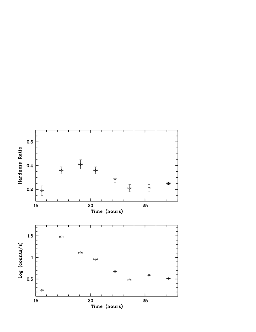
Figure 2: Hardness ratio and background subtracted light curve (in the 0.1–2.4 keV band) for the ROSAT PSPC observation. The hardness ratio is defined as H-S/H+S where H are the counts in the band between 0.1–0.28 keV and S the counts in the band between 0.5–2.0 keV. The resulting e–folding time of the light curve is $\tau_{\rm lc}=10.1\pm 0.5$ ks. For comparison, the hardness ratio measured during the RASS observations is $-0.04\pm 0.07$.

Fig. 2 shows the hardness ratio and background subtracted light curve for all the ROSAT pointings. Surprisingly, the hardest observation is that correspondent to the pointing number 201000, already in the flare decay phase. This issue will be discussed later in the context of the flare spectral analysis (Sect. 4.2). The light curve after the flare maximum can be well fitted by an exponential with e–folding decay time of $\tau_{d}\sim 10.1$ ks.

The RASS ROSAT observation performed during the first half of 1990 allows a comparison with the pre–flare (200998) and post–flare (201003, 201004, and 201005) pointings. The count rate of the RASS observation is $\sim 50\%$ higher than during the pre–flare but almost a factor 2 lower than during the last three observations whereas the hardness ratio ($-0.04\pm 0.07$) seems to indicate a softer status than those observed in November 1992. Intrinsic long–term variability both in count–rate and spectral shape thus emerges (see also the ASCA light curve, Sect. 3.2, and the spectral analysis of the quiescent emission, Sect. 4.1).

3.2 ASCA light curve

Gl 355 was observed by the ASCA satellite on 1993, May 7 at 20:14, roughly six month after the ROSAT observation. The effective exposures were 19.1 and 22.2 ks long for the SIS and GIS detectors, respectively. The sequence number of the observation is 21020000 and again we retrieved the raw data from the ASCA public archive.

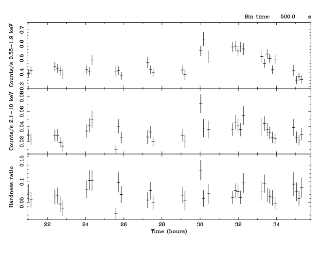
Figure 3: SIS0 light curves (not background subtracted) integrated in the energy bands 0.55-1.9 keV (top), 2.1–10 keV (middle), and the related hardness ratio (bottom). Observations were performed starting on 1993, May 7.

The light curves (Figure 3) were integrated considering two energy bands between 0.55–1.9 keV and 2.1–10 keV. The count rate is essentially constant for the first half of the observation, $\sim 0.4$ cts for the SIS. The second half, on the contrary, shows an increase of $\sim 50$% in particular in the softest band. However, the hardness ratio does not show significant variations due to the relatively poor statistics involved.

3.3 ROSAT spectra

The high ROSAT count rate allowed us to perform a time–resolved spectral analysis. We applied the optically thin plasma codes of Raymond & Smith (RS77 (1977)) and Mewe et al. (1996a , MEKAL). Both codes adopt optically–thin, collisional ionization equilibrium emissivity models. Since no significant differences were found in the results obtained with the two models we only report the MEKAL ones. The presence of absorbing material has been taken into account using the WABS component in XSPEC, which implements the Morrison & McCammon (MM83 (1983)) model of X–ray absorption from interstellar material. Abundance variations in the source spectra have been modeled through a single parameter, the global “metallicity” $Z$, by assuming a fixed ratio between individual elemental abundances and the corresponding solar photospheric values as given by Anders & Grevesse (AG89 (1989)).

The errors on the counts have been taken into account by the Gehrels (Geh86 (1986)) approximation for data following the Poissonian statistics rather than the Gaussian statistics. Systematic errors were also considered for the ROSAT data as discussed later. The $\chi^{2}$ minimization statistics was applied through the paper.

ROSAT spectra were extracted from the event files using the XSELECT/FTOOLS package and were rebinned to give at least 25 counts per bin. For all the observations a source spectrum was accumulated from a circular region of about $2\div 3$ arcmin, while a background spectrum was integrated in an annular region centered on the source with inner and outer radii of 4 and 11 arcmin, respectively. We also use the spectra produced automatically by the WGA catalog analysis procedures. In both cases the derived fit parameters were essentially the same. Being Gl 355 a relatively bright and isolated X–ray source, the automatic extraction procedure used in the WGA catalog processing produced accurate results.

The spectra for the individual ROSAT pointings were fitted with 1– and 2–temperature models, with variable $N_{\rm H}$ and metallicity $Z$. No attempt was made to vary the abundances of individual elements, since this is not warranted by the PSPC low–resolution.

For the observations with higher count rates (i.e. during the main part of the flare) we did not get any satisfactory spectral fit taking into account the Poissonian errors only, and no significant improvements could be obtained by adding further thermal components. In low–resolution spectra, such as those provided by the PSPC, high $\chi^{2}_{\rm red}$ values are unlikely to be due to uncertainties in the model. Coronal spectra obtained by ROSAT have in fact been widely fitted successfully. We rather interpret this result as a consequence of the high statistics of our spectra during the flare evolution which leads to Poissonian errors comparable to or less than the other sources of uncertainty. In particular, a calibration error of $\sim 2\%$ is expected to affect on average each spectral channel and we took it into account (Fiore et al. FEMSW94 (1994), Bocchino et al. BMS94 (1994)).

3.4 ASCA spectra

The extracted ASCA spectra were rebinned to give at least 25 counts per bin. For the SIS detectors, we used the standard background data provided by the ASCA observatory team since the source almost completely fills the 1–CCD mode FoV. Standard screening was applied and spectra were accumulated in a region as wide as possible around the source: 3 and 2 arcmin for SIS0 and SIS1, respectively. The GIS spectra were integrated in a region containing 98% of the source flux. A background spectrum was accumulated from the outer regions of the FoV.

To avoid known ASCA calibration problems, the spectral analysis was restricted to the energy range 0.55-10 keV for the SIS detectors and 0.6–10 keV for the GIS detectors. In fact, spectral channels at higher energies are dominated by the noise due to the rapid effective area decrease, while SIS channels with energy less then 0.55 keV have relevant calibration uncertainties (Dotani et al. DYR95 (1995)). No acceptable fit, in fact, was obtained including the low–energy channels both in terms of $\chi^{2}$ values and of the distribution of residuals.

We have performed spectral fits of ASCA data for the SIS0, SIS0+SIS1, GIS2, GIS2+GIS3, and SIS0+GIS2 datasets. SIS0 and GIS2 are the best calibrated detectors. The fits to these data were performed with 1–, 2– or 3–temperature models and free metallicity $Z$. Only in the case of the SIS spectra we have also performed the analysis with individual elemental abundances left free to vary. In all fits, in order to reduce the number of free parameters, the interstellar absorption $N_{\rm H}$ was fixed at $4\times 10^{19}$ cm^-2, as suggested by the ROSAT analysis (Sect. 4.1). However, due to the harder ASCA energy band, the adopted value of the absorbing column does not affect the results.

4 Results

4.1 Quiescent Emission

The ROSAT observations 200998 (the pre–flare observation), 201003, 201004, 201005, the ASCA observation and the RASS data allow us to study the quiescent emission of Gl 355 on a long and a short time–scale. As already pointed out in Sect(s). 3.1 and 3.2 on the basis of the light curves, both long– and short–term variability is clearly present amounting to up a factor of $2\div 3$ in flux.

Obs.	$N_{H}$	$KT$	EM	$Z$	flux${}_{0.1-2.4\,{\rm keV}}$	$\chi_{\nu}^{2}$	d.o.f.
	($10^{19}$ cm-2)	keV	$10^{52}$ cm-3	$Z/Z_{\odot}$	erg s-1 cm-2
200998n00	$4.20\pm^{3.16}_{2.63}$	$0.63\pm^{0.08}_{0.08}$	9.04	$0.08\pm^{0.04}_{0.03}$	$1.43\times 10^{-11}$	0.22	14
201003n00	$3.60\pm^{2.08}_{1.84}$	$0.76\pm^{0.07}_{0.06}$	14.53	$0.09\pm^{0.03}_{0.03}$	$2.58\times 10^{-11}$	1.3	14
201004n00	$4.70\pm^{1.88}_{1.72}$	$0.88\pm^{0.11}_{0.09}$	21.39	$0.05\pm^{0.03}_{0.02}$	$3.5\times 10^{-11}$	1.2	14
201005n00	$3.13\pm^{2.04}_{1.79}$	$0.75\pm^{0.07}_{0.06}$	14.93	$0.10\pm^{0.04}_{0.03}$	$2.79\times 10^{-11}$	1.3	14

Table 3: 1T fits to the ROSAT spectra for the quiescent emission. Errors at 90% confidence for the parameters of interest.

We have tried to fit the ROSAT PSPC observations on Nov 1992 with the simplest possible model: a 1T model with free global metallicity. No observation could be fitted with solar metallicity even assuming 2T and 3T models. As reported in Table 3, the first model gives acceptable fits. The absorbing column on the line of sight is not well constrained (errors of the order of 50% of the best fit value, or larger), but the mean value is $\sim 4\times 10^{19}$ cm^-2 and we could not obtain satisfactory fits with $N_{\rm H}$ lower than a few times $10^{19}$ cm^-2.

Figure 4: (Top) ROSAT spectrum for observation 200998 (the pre–flare observation). The best fit 1T model (Table 3) and fit residuals are also shown. (Bottom) ROSAT spectrum for observation 200999 (the flare peak). The best fit 2T model (Table 5) and fit residuals are also shown.

The metal abundance is highly subsolar ($Z/Z_{\odot}=0.03\div 0.14$ at the 90% confidence level) and is confirmed by the analysis of the ASCA spectra discussed below. The best–fit temperature is $\sim 0.7$ keV with a moderate hardening for observation 201004 coincident with the small flare apparently superimposed to the tail of the main event (Fig. 1). The flux in the 0.1–2.4 keV energy band ranges from $\sim 1.4$ to $\sim 3.5\times 10^{-11}$ erg cm^-2s^-1, directly linked to the EM variations from $\sim 9$ to $\sim 21\times 10^{52}$ cm^-3. All ROSAT observations outside of the flare can thus be fitted by 1T models (see the best fit for observation 200998 in Fig. 4, top panel). The spectral parameters derived for the pre– and post–flare emissions are comparable and the moderate (a factor of $2\div 3$) flux variability seems to be due mainly to EM variations which in turn might be due to changes in either the volume or the density of the emitting regions.

Camera	KT1	EM1	KT2	EM2	Z	flux${}_{0.55-10\,{\rm keV}}$	$\chi_{\nu}^{2}$	d.o.f.
	keV	$10^{52}$ cm-3	keV	$10^{52}$ cm-3	$Z/Z_{\odot}$	erg s-1 cm-2
SIS0	$0.65\pm^{0.05}_{0.09}$	4.44	$1.30\pm^{0.34}_{0.27}$	3.23	$0.15\pm^{0.07}_{0.05}$	$1.10\times 10^{-11}$	0.9	103
SIS0+SIS1	$0.62\pm^{0.01}_{0.07}$	4.44	$1.17\pm^{0.21}_{0.15}$	3.63	$0.13\pm^{0.05}_{0.03}$	$1.10\times 10^{-11}$	0.9	203
GIS2	$0.87\pm^{0.10}_{0.09}$	6.46	-	-	$0.11\pm^{0.07}_{0.04}$	$0.81\times 10^{-11}$	0.8	111
GIS2+GIS3	$0.89\pm^{0.07}_{0.06}$	6.46	-	-	$0.12\pm^{0.05}_{0.03}$	$0.83\times 10^{-11}$	0.8	245
SIS0+GIS2	$0.65\pm^{0.04}_{0.06}$	4.44	$1.39\pm^{1.60}_{0.27}$	2.42	$0.17\pm^{0.08}_{0.05}$	$1.00\times 10^{-11}$	1.1	217

Table 4: 1T and 2T fits to ASCA spectra. For simultaneous fits the normalizations are kept the same for both SIS and GIS detectors. Errors at 90% confidence for the parameters of interest.

Considering the ASCA observation on May 1993 1T spectral fits gave satisfactory results only for the low resolution GIS detectors. The best fit temperature appears slightly harder (but comparable within the errors) than that one derived from the ROSAT analysis, while the metal abundance is essentially the same (Table 4).

Obs.	$N_{H}$	$KT_{1}$	EM1	$KT_{2}$	EM2	$Z$	flux0.1-2.4keV	$\chi_{\nu}^{2}$	d.o.f.
	$(10^{19}$ cm-2)	keV	$10^{52}$ cm-3	keV	$10^{52}$ cm-3	$Z/Z_{\odot}$	erg s-1 cm-2
200999n00	$1.87\pm^{1.76}_{1.54}$	$0.71\pm^{0.23}_{0.26}$	8.76	$4.44\pm^{n.c.}_{1.53}$	114.30	$0.55\pm^{0.80}_{0.45}$	$3.11\times 10^{-10}$	1.0	12
201000n00	$2.80\pm^{2.31}_{2.20}$	$0.53\pm^{0.20}_{0.19}$	4.84	$2.69\pm^{2.29}_{0.76}$	41.17	$0.62\pm^{1.20}_{0.38}$	$1.28\times 10^{-10}$	0.9	12
201001n00	$2.83\pm^{2.21}_{2.07}$	$0.61\pm^{0.23}_{0.29}$	8.88	$1.65\pm^{n.c.}_{0.40}$	25.51	$0.28\pm^{0.40}_{0.17}$	$8.45\times 10^{-11}$	0.9	12
201002n00	$2.72\pm^{2.71}_{2.32}$	$0.61\pm^{0.17}_{0.29}$	7.67	$1.75\pm^{n.c.}_{1.43}$	10.90	$0.21\pm^{0.35}_{0.12}$	$4.22\times 10^{-11}$	0.5	12

Table 5: 2T ROSAT MK fits for the flare emission. The metal abundance is free to vary in solar proportion. Errors at 90% confidence for the parameters of interest.

Acceptable fits to the SIS spectra were obtained only with the addition of a second thermal component, with the global metallicity free to vary (Table 4). The metal abundance is comparable to that obtained from the analysis of the ROSAT data and is well below solar. Since ASCA is much more effective than ROSAT in measuring metal abundances, this result clearly shows that a low metal abundance is indeed needed to model the corona of Gl 355 in spite of the fact that this is a very young star with presumably solar photospheric abundances. As expected, the introduction of a second component gives a lower value for the cooler temperature, while the hotter temperature is around $1.3$ keV and its EM is about 25–50% lower than that one of the cooler component. The higher temperature derived for the ASCA 2T fit is due to the much larger energy range involved, which makes ASCA sensitive to hotter plasma than the ROSAT PSPC.

		SIS0	SIS0+SIS1
$KT_{1}$	(keV)	$0.64\pm^{0.00}_{0.03}$	$0.63\pm^{0.02}_{0.030}$
EM1	($10^{52}$ cm-3)	3.96	4.44
$KT_{2}$	(keV)	$2.10\pm^{0.70}_{0.30}$	$2.00\pm^{0.40}_{0.30}$
EM2	($10^{52}$ cm-3)	1.53	1.61
O${}_{(FIP=13.6\,eV)}$		$0.47\pm^{0.30}_{0.19}$	$0.39\pm^{0.17}_{0.13}$
Ne${}_{(FIP=21.6\,eV)}$		$0.65\pm^{0.36}_{0.24}$	$0.55\pm^{0.21}_{0.16}$
Mg${}_{(FIP=7.6\,eV)}$		$0.32\pm^{0.23}_{0.15}$	$0.24\pm^{0.13}_{0.10}$
Si${}_{(FIP=8.2\,eV)}$		$0.33\pm^{0.18}_{0.15}$	$0.31\pm^{0.12}_{0.10}$
S${}_{(FIP=10.4\,eV)}$		$0.50\pm^{0.42}_{0.38}$	$0.41\pm^{0.27}_{0.25}$
Fe${}_{(FIP=7.9\,eV)}$		$0.17\pm^{0.09}_{0.05}$	$0.15\pm^{0.05}_{0.04}$
$\chi^{2}_{\nu}$	(d.o.f. = 98)	0.7	0.7
flux${}_{0.55-10\,{\rm keV}}$	erg s-1 cm-2	$1.2\times 10^{-11}$	$1.2\times 10^{-11}$

Table 6: 2T fits to ASCA spectra with individual abundances free to vary. For simultaneous fits the normalizations are kept the same for both SIS cameras. Errors at 90% confidence for only one parameter of interest.

In order to study in detail the chemical composition of stellar coronal plasmas several authors have fitted ASCA spectra with thermal models in which the elemental abundances are allowed to vary individually, rather than in a fixed ratio with respect to the solar values (e.g. White et al. WAD94 (1994), Drake et al. DSWS94 (1994), Mewe et al. 1996b , Tagliaferri et al. TCF97 (1997), Ortolani et al. OMP97 (1997)). We have tried the same approach for the SIS0 and SIS0+SIS1 datasets (Table 6) considering as free parameters only the ions that contribute most to line emission in the ASCA passband. These include O, Ne, Mg, Si, S and Fe, whose abundances can be sufficiently well constrained. Similar fits made by adding N, Ar and Ca as free parameters resulted in essentially unconstrained abundances for these elements. The abundances of all other elements were frozen to their solar values (see Mewe et al. MKvVT97 (1997) for a discussion).

Satisfactory fits were obtained with 2T models (Table 6). The hotter temperature is harder than that obtained with 2T fits and a variable global metallicity, while the ratio between the two EM is lower by $\sim 40$%. This is likely due to the redistribution of the best fit element abundances which, although all below solar, show a significant lower iron abundance with respect to solar than the other elements. Note however that the fit with variable individual abundances is not statistically better than the one with a single global metallicity.

Finally, we have tried to fit the SIS spectra with 3–temperature (3T) models and solar abundances. These fits still did not give satisfactory results. The addition of a third component simply redistributed the temperature over a wider range. If the global metallicity is left free to vary both the SIS0 and the SIS0+SIS1 data sets gave satisfactory results but the introduction of a further thermal component is not formally required by the fit.

4.2 Flare analysis

In order to analyze the flare emission it is necessary to separate it from the quiescent emission of the corona. In the previous section we have shown that the definition of a “quiescent spectrum” for Gl 355 is not straightforward since a significant amount of variability is present. Considering the ROSAT observations 200999, 201000, 201001 and 201002, i.e. the observations performed during the flare, no satisfactory fit could be obtained with 1T models. Even subtracting the ROSAT observation 200998, or an average of the three post–flare observations 201003, 201004 and 201005, no adequate fit could be obtained. We thus performed 2T fits with the global metallicity either fixed to the solar value or left free to vary. With solar metallicity the fits are worse than the corresponding fits with 1T and global metallicity free to vary. However, if we allow the metal abundance to vary, the 2T fits give acceptable results (Table 5 and Fig. 4, bottom panel), but the hotter component is badly constrained. No better constraining can be obtained by freezing the absorbing column and/or fixing the metal abundance to the quiescent value. The intense dynamic evolution of the flare prevents a detector with a limited energy band as the ROSAT PSPC to constrain the hot component.

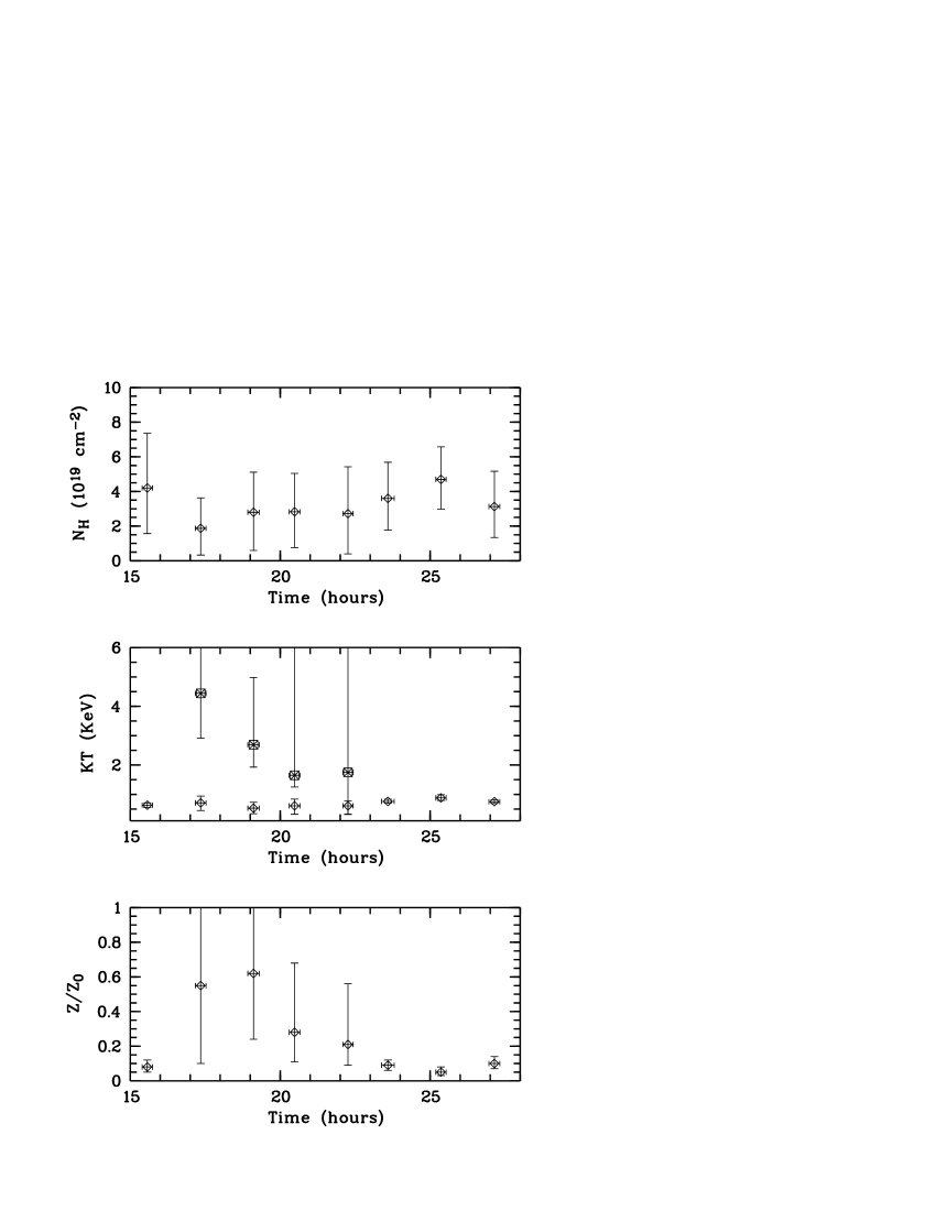
Figure 5: 1 and 2–T best fit parameters for the ROSAT PSPC observations. The first observation and the last three were fitted by 1T models, while the observations performed during the flare were fitted with 2T models (see Fig. 1).

As shown in Fig. 5, the temperature of the flare cooler component is essentially constant around 0.6–0.7 keV, in full agreement with the temperature derived for the quiescent emission.

The absorbing column density is also essentially constant during the flare, i.e. with no increase at the flare onset or at the peak which, if present, could be interpreted as evidence for a mass ejection. The metal abundance close to the flare peak is not well constrained but a hint (admittedly very weak) for an increase during the flare evolution seems to be present (Fig. 5).

In any case a hot component is clearly needed, although being not well constrained due to the limited ROSAT energy range. The flare event is totally due to hot plasma superimposed to the quiescent corona.

We note in passing that the observation 201000 shows for the low temperature component the lowest EM among the flare observations, about half of the values obtained for observations 200999, 201001 and 201002. The temperature is slightly reduced. These two factors likely explain why the hardness ratio for this observation is the hardest during the flare (cf. Table 2 and Fig. 2). This phenomenum may also be related to the presence of heating during the decay phase of the flare discussed in Sect. 5.

5 Flare modeling

5.1 Loop modeling

The flare observed by ROSAT has been analyzed considering the so called hydrodynamic decay–sustained heating scenario (Reale et al. RBPSM97 (1997)), which assumes that the flaring plasma is confined in a closed loop structure whose geometry does not change during the event. This method simultaneously yields estimates for the size of the flaring loop as well as for the presence and time scale of heating during the decay phase of the flare. The method uses the slope of the locus of points in the temperature vs. density diagram of the flare decay phase which, from hydrodynamic simulations of X–ray flares, has been found to be a good diagnostics for the presence of sustained heating. Under the assumption that the loop volume remains constant during the flare, the square root of the emission measure can be used as an indicator for the density. We also assume that the flare loop length is small in comparison with the coronal pressure scale height i.e. that isobaric conditions hold for the plasma in the flaring loop (we will verify the correctness of this assumption a posteriori). For the present flare, we make the further assumption that the hot component found in the 2T fits discussed in the previous section is indeed responsible for the flare event (i.e. that the cool component contributes only to the quiescent emission).

Detailed hydrodynamical simulations (Peres et al. PSVR82 (1982), Betta et al. BPRS97 (1997)) show that flares decay approximately along a straight line in the $\log\sqrt{EM}-\log T$ diagram, and that the value of the slope $\zeta$ of the decay path is related to the ratio between the observed decay time $\tau_{\rm lc}$ of the light curve and the thermodynamic cooling time of the loop $\tau_{\rm th}$ in the absence of heating during the flare decay. This allows deriving the length of the flaring loop as a function of observable quantities. Since the characteristics of the observed decay depend on the instrument response, the specific relationships to be used depend on the instrument and must be appropriately calibrated. An application of this technique to stellar flares observed with the ROSAT PSPC, and the appropriate calibrations, are given by Reale & Micela (RM98 (1998)) and Favata et al. (2000c ). See also Pallavicini et al. (1999) for a critical discussion of the method.

The theoretical thermodynamic decay time $\tau_{\rm th}$ (sec) of a closed coronal loop with semi–length $L$ (cm), and maximum temperature $T_{\rm max}$ (K) in the absence of sustained heating is (Serio et al. SRJSS91 (1991)):

$$\tau_{\rm th}=\frac{\alpha L}{\sqrt{T_{\rm max}}}$$ (1)

where $\alpha=3.7\times 10^{-4}$ cm^-1 s K^1/2. By means of a grid of hydrostatic loop models, an empirical relationship linking the loop maximum temperature $T_{\rm max}$ to the temperature $T_{\rm obs}$ (K) has been derived:

$$T_{\rm max}=0.13\times T_{\rm obs}^{1.163}.$$ (2)

In the present case, we cannot be sure that the flare maximum was observed but we can assume that the observation 200999 is not too far from the real flare peak. The observed peak temperature is $51.5\pm^{n.c.}_{17.7}\times 10^{6}$ K and therefore the actual maximum temperature from Eq. (2) is $\sim 121\times 10^{6}$ K.

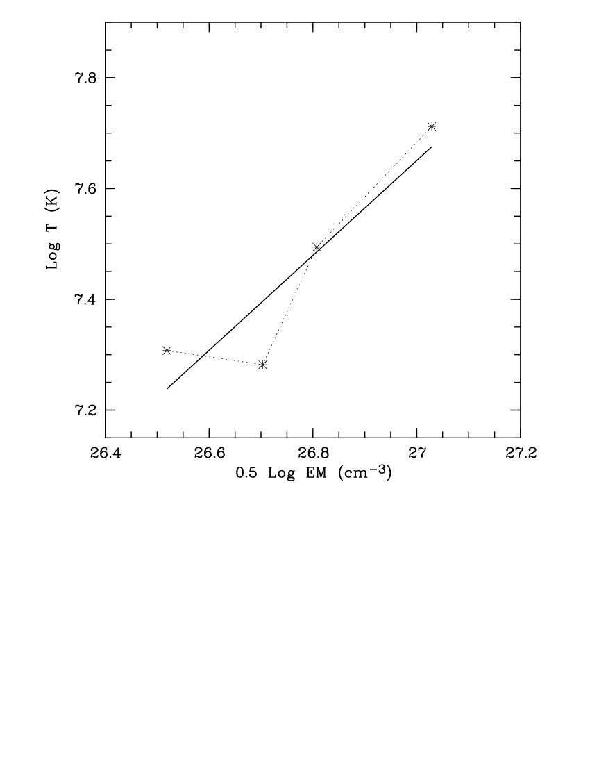
Figure 6: The evolution of the flare decay in the $\log T$ vs. $\log\sqrt{EM}$ plane. The dotted line connects points in temporal order while the solid line is the best fit to the decay.

The ratio between $\tau_{lc}$ and $\tau_{th}$ is a function of the slope $\zeta$ in the $\log\sqrt{EM}-\log T$ (see Fig. 6). The best fit for $\zeta$ with the present data is $0.86\pm 0.27$.

Applying the relation reported for the ROSAT data by Favata et al. (2000c ) valid for $0.4\leq\zeta\leq 1.7$:

$$\frac{\tau_{\rm lc}}{\tau_{th}}=F(\zeta)=\frac{3.67}{\zeta/0.3-1.0}+1.61$$ (3)

we get $F(\zeta)=3.6\pm 0.9$ with the value of the slope $\zeta$ derived above. Very low values of $\zeta$ mean that the flare decay is entirely driven by the sustained heating, so that the thermodynamic cooling time, $\tau_{\rm th}$, cannot be determined in a reliable way, and $L$ does not depend any more on $\tau_{\rm lc}$. On the other extreme, no sustained heating occurs and $\tau_{\rm lc}\sim\tau_{\rm th}$. The case discussed here is in the right regime where to apply Eq. (3). Our result shows that a large amount of sustained heating is actually present in line with the results obtained for other flares (Reale & Micela RM98 (1998); Ortolani et al. OPMRW98 (1998), Favata & Schmitt FS99 (1999); Favata et al. 2000a ; Favata et al. 2000b ; Favata et al. 2000c ; Maggio et al. MPRT00 (2000), Franciosini et al. Fetal01 (2001)).

The expression for the loop semi–length $L$ is:

$$L=\frac{\tau_{\rm lc}\sqrt{T_{\rm max}}}{\alpha F(\zeta)},$$ (4)

For the present event, the decay e–folding time, $\tau_{\rm lc}$ is $10.1\pm 0.5$ ks, and with the values above for $T_{max}$ and $\zeta$, the loop semi–length turns out to be $L=83(\pm 22)\times 10^{9}$ cm or, in units of the stellar radius, $L\sim 1.5\,R_{*}$. The uncertainty on $L$ is given by the sum of the propagation of the errors on the observed parameters $\tau_{\rm lc}$ and $\zeta$ with the standard deviation of the difference between the true and the derived loop lengths. The latter uncertainty, estimated by applying the method to spatially resolved observations of solar flares, amounts to $\approx 20\%$ and usually dominates on the other error sources. The loop length derived here could be somewhat underestimated if the flare peak occurred earlier than observation 200999, i.e. at a time when we had a data gap. The above relationships have been derived in the assumption of negligible interstellar absorption ($N_{\rm H}\sim 0$) and solar metallicity, but the corrections are small provided $N_{\rm H}\leq 10^{20}$ cm^-2 (Reale & Micela RM98 (1998)) and the metal abundance is at least of the order $Z/Z_{\odot}\sim 0.1$: these conditions are satisfied in our case.

The derived loop size is small in comparison with the pressure scale height, thus justifying the initial assumption that the flaring loops are isobaric. In fact, the pressure scale height is $H=2KT/\mu g$, where $T$ is the plasma temperature in the loop, $\mu$ is the molecular weight and $g$ is the surface gravity of the star. With $\log g/g_{\odot}\sim 0.07$ and $\mu\sim 0.6$ we get $H\sim 6\times 10^{11}$ cm.

The average plasma density can be estimated as:

$$n_{e}\sim\sqrt{\frac{EM}{V}},$$ (5)

where $EM$ is the emission measure derived from the fit, and $V$ the loop volume. Assuming $\beta=0.1\div 0.3$ for the ratio between the radius of the loop cross–section and its semi–length (typical values for solar coronal loops, Golub et al. GMR80 (1980)) we obtain $V=2\pi L^{3}\beta^{2}=3.6\div 33\times 10^{31}$ cm³ (considering the uncertainties on $\beta$ and $L$). Eq. (5) thus yields $n_{\rm e}=2\div 0.7\times 10^{11}$ cm^-3. The corresponding pressure $p_{e}=2n_{\rm e}kT_{\rm max}=6.7\div 2.3\times 10^{3}$ dyne cm^-2.

Using the scaling laws of Rosner et al. (RTV78 (1978)) applicable to static loops $T_{\rm max}=1.4\times 10^{3}(p_{0}L)^{1/3}$ K, where $p_{0}$ is the pressure at the base of the loop, we derive, at the temperature peak, $p_{0}=7.7\times 10^{3}$ dyne cm^-2. The similarity of $p_{0}$ and $p_{e}$, for the adopted range of values for $\beta$, implies that the plasma at the flare peak is not far from quasi-static conditions, i.e. the loop is almost completely filled with plasma evaporated from the chromosphere, as a consequence of the heating.

Obs.	$L_{X_{(0.1\div 2.4\,{\rm KeV})}}$	$L_{X_{(0.1\div 2.4\,{\rm KeV})}}$
	erg s-1	erg s-1	$L_{\rm flare}/L_{X}$
	total	flare only
RASS	$8.50\times 10^{29}$
200998n00	$5.77\times 10^{29}$
200999n00	$1.25\times 10^{31}$	$1.09\times 10^{31}$	0.87
201000n00	$5.10\times 10^{30}$	$4.16\times 10^{30}$	0.82
201001n00	$3.40\times 10^{30}$	$2.34\times 10^{30}$	0.69
201002n00	$1.70\times 10^{30}$	$0.93\times 10^{30}$	0.55
201003n00	$1.00\times 10^{30}$
201004n00	$1.35\times 10^{30}$
201005n00	$1.08\times 10^{30}$

Table 7: X–ray flare luminosity evolution. For comparison the luminosity detected during the RASS observation and for the pre– and post–flare quiescent emissions are also reported. In Column 2 the total luminosity from Gl 355 is reported; in Column 3 the luminosity of the flare component only and, finally, in Column 4, the fraction of the total luminosity due to the flare component.

It is interesting to compute the coronal magnetic field strength required to keep confined a plasma with the density reported here. Equating the magnetic pressure to the gas pressure in the flaring loop, $B^{2}/8\pi\sim p_{e}$, we get a value of $\sim$ 300 G in the corona. If we assume that the magnetic field has a dipolar structure, i.e. it scales with height with a $r^{-3}$ law, the expected magnetic field at the stellar surface in the flaring region comes out to be of the order of 2500 G. Recently, Donati (D99 (1999)) studied the magnetic cycles of HR 1099 and Gl 355 by means of Zeeman–Doppler imaging, and reported evidences for large–scale magnetic fields on Gl 355 with strengths of up to a few hundred Gauss. This discrepancy could mean that either the large scale magnetic field studied by Donati (D99 (1999)) is not related to the localized fields responsible for large flares or that the structure of these localized fields is not dipolar. In any case, conventional Doppler imaging measurements show that magnetic fields of the order of a few thousands Gauss are not uncommon on late–type active stars as AD Leo (see for instance Saar & Linsky SL85 (1985) and Linsky & Saar LS87 (1987)). We stress, however, that within the hypothesis of dipolar fields, the inferred strength of the photospheric magnetic field is not significantly affected by the derived flare loop size because a smaller loop implies a higher gas and magnetic pressure in the corona, but also a smaller difference between the strength of the photospheric and coronal magnetic fields. For instance, if the flare loop were a factor ten smaller, we would still require a photospheric magnetic field of about 2200 G in the dipole approximation.

Finally, we have computed, for each time interval during the flare, the X–ray luminosity in the $0.1\div 2.4$ keV band (see Table 7). A detailed determination of the energy balance of the present flare is not possible given the lack of multi-wavelength coverage and velocity information which could help assessing the plasma kinetic energy. The Gl 355 bolometric luminosity is $\sim 1.8\times 10^{33}$ erg s^-1. The total energy radiated by the flare in X–rays in the band $0.1\div 2.4$ keV is $E\sim 9\times 10^{34}$ over $\sim 19$ ks, and is equivalent to $\sim 0.4$% of the star’s bolometric energy output during the same interval. The observed peak flare luminosity was $\sim 1$% of the star’s bolometric luminosity.

5.2 “Order of magnitude” estimates

It is interesting to compare the above results, based on self-consistent hydrodynamic loop models, with simple order of magnitude estimates of the radiative and conductive cooling times for a single flaring loop with no additional heating in the decay phase. This approach is the one that has been most commonly used in previous analyses of stellar flares. We follow here the formalism of Pallavicini (P95b (1995); see also Pallavicini et al. PTS90 (1990)). For a loop of density $n_{e}$ and temperature $T$, the radiative cooling time is given by:

$$\tau_{\rm rad}=\frac{3kT}{n_{e}P(T)}$$ (6)

where $k$ is the Boltzmann constant and P(T) is the radiative loss function for unit emission measure which can be approximated as $P(T)\simeq 10^{-24.73}T^{0.25}$ erg cm³ s^-1 for temperatures higher than 20 MK (Mewe et al. MGv85 (1985)). If the flare cools predominantly by radiation, the above equation, together with the flare coronal temperature derived from the spectral fits (see Table 6), allows deriving a value for the flare density (or only an upper value to it, if conduction is not negligible). With $T=51.5\times 10^{6}$ K, this gives $n_{e}=1.3\times 10^{11}$ cm^-3, which, from Eq. (5), results in a volume (or in a lower limit to it) of $6.8\times 10^{31}$ cm³. With $\beta$ in the range $0.1\div 0.3$, the loop semi–length is thus $L\sim 100\div 50\times 10^{9}$ cm. i.e. slightly larger than the stellar radius and comparable to the values inferred above from the hydrodynamic modeling.

As discussed by Haisch (1983, see also Pallavicini 1995), if conduction losses are not negligible, but are comparable to radiative losses, it is possible to determine uniquely the loop length (as opposite to determining only an upper limit to it), under the assumption again that there is no heating during the flare decay. In fact, the conductive cooling time is given by:

$$\tau_{\rm cond}=4.8\times 10^{-10}\frac{n_{e}L^{2}}{T^{2.5}}$$ (7)

which, for $\tau_{\rm cond}\sim\tau_{\rm rad}$, gives $L=56\times 10^{9}$ cm, which is again comparable to the stellar radius in the case of Gl 355. Finally, we note that the so-called quasi-steady cooling model (van den Oord and Mewe vM89 (1989)), often used in modeling stellar flares, coincides, for the radiative loss function $P(T)$ assumed above, to a ratio $\tau_{\rm rad}/\tau_{\rm cond}=0.18$, i.e. to the case of radiation dominated cooling, although conduction is not completely negligible. Hence, the loop length estimated from the quasi-static cooling model cannot be too different from that estimated from radiative cooling alone (Pallavicini P95b (1995)).

Due to the similarity between the estimates of the Gl 355 flare loop size performed with the Reale et al. (RBPSM97 (1997)) approach and with simple “order of magnitude” considerations, we also analyzed four flares from Algol (Favata et al. 2000c ), three flares from AB Dor (Franciosini et al. Fetal01 (2001)), one more flare from AB Dor (Ortolani et al. OPMRW98 (1998)), six flares from AD Leo (Favata et al. 2000b ) and one flare from EV Lac (Favata et al. 2000a ).

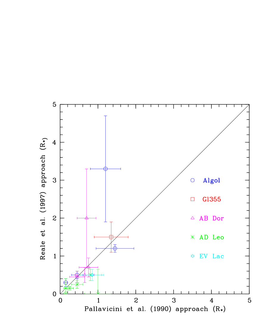
Figure 7: Comparison between flares loop sizes determined by the methodology developed by Reale et al. (RBPSM97 (1997)) and by the “order of magnitude” estimates by Pallavicini et al. (PTS90 (1990)).

The result of this comparison is shown in Fig. 7. In spite of the fact that simple orders of magnitude estimates are clearly based on physically wrong assumptions (since evidences of sustained heating during the decay of the considered flares have been usually reported), they provide values for the flare volume and density which are not too dissimilar from those derived from the hydrodynamic decay-sustained heating model of Reale et al. (RBPSM97 (1997)). Moreover, in many cases, the loop semi–length derived with both methods is large and comparable to the stellar radius, a situation quite different from that encountered in the case of solar flares. The large flare size is clearly needed to provide the large energy release of stellar flares with respect to solar ones, without requiring unrealistically high values of the magnetic field.

Several factors are probably conspiring here to give us this surprising coincidence. On one hand it is well known that if there is evidence of heating in the flare decay, the use of the observed quantity $\tau_{\rm lc}$ instead of the theoretical $\tau_{\rm th}$ to estimate the flare sizes, intrinsically produces too large loop lengths. On the other hand, if we assume that there is no heating, the density estimated from radiative cooling only should be higher than the true values since the flare also cools by conduction and the volume derived is correspondingly lower.

Within the limits of the small sample analyzed here, no trend seems to emerge for flare size with respect to the star parameters as spectral types, rotation rates, etc.

6 Summary and conclusions

The spectral analysis of the ROSAT and ASCA data show that this young star has coronal metal abundances strongly sub–solar. Although there are no direct measurements of the photospheric abundances of Gl 355, it is expected to be solar. Thus, as in the case of other young objects, e.g. AB Dor (Mewe et al. 1996b ) and HD 35850 (Tagliaferri et al. TCF97 (1997)), we have a star that shows coronal abundances much lower than the photospheric ones. This is also true for other more evolved stars, as e.g. II Peg (Mewe et al. MKvVT97 (1997); Covino et al. CTPMP00 (2000)). These ROSAT, ASCA and BeppoSAX findings are now confirmed with the gratings observations of Chandra for HR 1099 (Drake et al. DBK01 (2001)) and of XMM-Newton for AB Dor, Castor and HR 1099 (Brinkmann et al. BBG01 (2001), Güdel et al. 2001a , 2001b ).

Besides the strong flare detected by ROSAT, variability of a factor of 2-3 has been detected in both ROSAT and ASCA light curves of Gl 355. This variability is mainly due to EM changes, while the temperature of the quiescent corona remains approximately constant. For the ROSAT data, outside the flare, the coronal plasma is well represented by a single temperature model with very low metal abundances. For the ASCA data, due to the harder energy band, a second harder component is required.

Applying the relation $N_{\rm H}\sim 0.07$ cm^-3 from Paresce (P84 (1984)), and assuming a distance of $\sim 18$ pc for Gl 355, we obtain $N_{\rm H}\sim 4\times 10^{18}$ cm^-2. However, acceptable fits to the ROSAT data could only be obtained with $N_{\rm H}$ an order of magnitude higher. Fruscione et al. (FHJW94 (1994)), compiling a list of measured hydrogen column densities for stars mainly in the solar neighborhood, showed that for an object at slightly less than 20 pc $N_{\rm H}$ of the order of $10^{19}$ are possible (their Fig. 3). It has also been suggested (Rodonó et al. RPL99 (1999)) that extra–absorption might occur in some stars owing to the presence of neutral hydrogen in the circumstellar environment.

The most interesting feature in the Gl 355 ROSAT data is of course the strong flare detected. The coronal spectrum during the flare can be represented with a 2-T model, with the cooler component compatible with the quiescent one. From these fits we have a weak indication of an increase of the metal abundance during the flare although the large error bars do not allow for a strong claim. A change of the metal abundance value during strong flare was detected for various sources and with different satellites (e.g. Algol with ROSAT and BeppoSAX: Ottmann & Schmitt OS96 (1996), Favata & Schmitt FS99 (1999); AB Dor with XMM-Netwon: Güdel et al. 2001a ). A separate issue is whether a variation of the column absorption could occur during the flare. Enhancements of the hydrogen column density, associated with flaring events, have been observed in the past on Proxima Cen (Haisch et al. HLB83 (1983)), V773 Tau (Tsuboi et al. TKM98 (1998)) and Algol (Ottmann & Schmitt OS96 (1996); Favata & Schmitt FS99 (1999)), and usually interpreted as due to a coronal mass ejection. However, solar observations show that coronal mass ejection and flares are not always physically related one to another (Golub & Pasachoff GP97 (1997)). No evidence of mass ejection can be significantly singled out from the evolution of the best fit $N_{\rm H}$ in the present data.

We modeled the flare using the hydrodynamic decay–sustained heating scenario (Reale et al. RBPSM97 (1997)) and assumed that in the 2-T best fit model, the hotter temperature represents the flare plasma, while the cooler temperature represents the quiescent coronal plasma. We then derived the flare loop semi–length that turns out to be quite large, $\sim 1.5\,R_{*}$. Note that our flare temperature (the hotter component) in not well constrained at higher values, due to the ROSAT energy band. In any case, since the downward error bars for the temperature are well constrained by the fit, the loop semi–length that we derived should be regarded as a lower limit (in the Reale et al. RBPSM97 (1997) model scenario).

We then analyzed the flare with a simple “order of magnitude” approach (Pallavicini et al. PTS90 (1990), Pallavicini P95b (1995)) able to provide a lower limit for the loop semi–length since it considers only the radiative cooling time ignoring the conductive cooling and the continuous heating of the flare plasma. The lower limit for the loop semi–length so derived is however in agreement with that derived by the full hydrodynamic decay–sustained heating approach, in spite of the fact that the two techniques are based on quite different assumptions.

We then applied this approach to various flares already analyzed by different authors using the Reale et al. (RBPSM97 (1997)) methodology. We considered four flares from Algol (Favata et al. 2000c ), three flares from AB Dor (Franciosini et al. Fetal01 (2001)), one flare from AB Dor (Ortolani et al. OPMRW98 (1998)), six flares from AD Leo (Favata et al. 2000b ) and one flare from EV Lac (Favata et al. 2000a ). It is interesting to note that these simple “order of magnitude” estimates, based on poorly justified and/or physically inconsistent assumptions, give again loop semi–lengths comparable to those derived with the Reale et al. (RBPSM97 (1997)) model. Apparently, the various assumptions made in the simplified “order of magnitude” approach (such as for instance that there is no heating during the flare decay or that the radiative to conductive losses have a fixed ratio) conspire to give loop sizes which are in gross agreement with the method based on detailed hydrodynamic calculations. On the other hand, the fact that the latter approach is based on physically sound assumptions give a much better confidence on the reliability of flare loop sizes derived in this way.

- (1) Ambruster C., Fekel F.C. 1990, BAAS 22, 857
- (2) Ambruster C.W., Sciortino S., Golub L., 1989, ApJS 65, 273
- (3) Anders E., Grevesse N 1989, Geochim Coschim. Acta 53, 197
- (4) Antunes A., Nagase F., White N.E. 1994, ApJ 436, L83
- (5) Basri G., Marcy G.W. 1994, ApJ 431, 844
- (6) Betta R., Peres G., Reale R., Serio S. 1997, A&AS 122, 585
- (7) Bocchino F., Maggio A., Sciortino S. 1994, ApJ 437, 209
- (8) Bowyer S., Lampton M., Lewis J., Wu X., Jelinsky P., Malina R.F. 1996, ApJS 102, 129
- (9) Brinkmann A.C., Behar E., Güdel M. et al. 2001, A&A, in press
- (10) Burke B.E., Mountain R.W., Harrison D.C., et al. 1991, IEEE Trans. ED–38, 1069
- (11) Covino S., Tagliaferri G., Pallavicini R., Mewe R., Poretti E. 2000, A&A 355, 681
- (12) Craig N., Abbott M., Finley D., et al. 1997, ApJS 113, 131
- (13) Culhane J.L., White N.E., Shafer R.A., Parmar A.N. 1990, MNRAS 243, 424
- (14) Day C., Arnaud K., Ebisawa K., et al. 1995, The ABC Guide to ASCA Data Reduction, NASA/GSFC
- (15) Donati J.–F. 1999, MNRAS 302, 457
- (16) Donati J.–F., Semel M., Carter B.D., Rees D.E., Cameron A.C. 1997, MNRAS 291, 658
- (17) Dotani T., Yamashita A., Rasmussen A. 1995, ASCA News 3
- (18) Drake J.J., Brickhouse N.S., Kashyap V. et al. 2001, ApJL, in press
- (19) Drake S.A., Singh K.P., White N.E., Simon T. 1994, ApJ 436, L87
- (20) ESA 1997, The Hipparcos and Tycho Catalogues, ESA SP-1200
- (21) Favata F., Micela G., Reale F. 2000b, A&A 354, 1021
- (22) Favata F., Micela G., Reale F., Sciortino S., Schmitt J.H.M.M. 2000c, A&A, in press
- (23) Favata F., Reale F., Micela G., et al. 2000a, A&A 353, 987
- (24) Favata F., Schmitt J.H.M.M. 1999, A&A 350, 900
- (25) Fekel F.C., Bopp B.W., Africano J.L., et al. 1986a, AJ 92, 1150
- (26) Fekel F.C., Hoffet T.J., Henry G.W. 1986b, ApJS 60, 551
- (27) Fiore F., Elvis M., McDowell J.C., Siemiginowska A., Wilkes B.J. 1994, ApJ 431, 515
- (28) Fleming T.A., Molendi S., Maccacaro T., Wolter A. 1994, ApJS 99, 701
- (29) Franciosini E., Pallavicini R., Maggio A., et al. 2001, ASP Conf. Ser., in press
- (30) Fruscione A., Hawkins I., Jelinsky P., Wiercigroch A. 1994, ApJS 94, 127
- (31) Gehrels N. 1986, ApJ 303, 336
- (32) Golub L., Maxson C., Rosner R., et al. 1980, ApJ 238, 343
- (33) Golub L., Pasachoff J.M. 1997, The Solar Corona, Cambridge University Press
- (34) Graffagnino V.G., Wonnacot D., Schaeidt S. 1995, MNRAS 275, 129
- (35) Grosso N., Montmerle T., Feigelson E.D., et al. 1997, Nat 387, 56
- (36) Güdel M., Audards M., Briggs K. et al. 2001, A&A, in press
- (37) Güdel M., Audards M., Magee H. et al. 2001, A&A, in press
- (38) Haisch B.M. 1983, in Activity in red–dwarf stars, IAU Coll. 71, eds. P.B. Byrne, M. Rodonò, Reidel, Dordrecht, 255
- (39) Haisch B.M., Linsky J.L., Bornmann P.L., et al. 1983, ApJ 267, 280
- (40) Haisch B.M., Rodonò M. 1989, Solar and Stellar Flares, “Proc. of IAU Colloquium No. 104” (Dordrecht: Kluwer Acad. Publ.)
- (41) Haisch B.M., Strong K.T., Rodonó M. 1991, ARA&A 29, 275
- (42) Hempelmann A., Schmitt J.H.M.M., Schultz M., Rüdiger G., Stephien K. 1995, A&A 294, 515
- (43) Huenemoerder D.P. 1998, ASP Conf. Ser. 154, 1061
- (44) Hünsch M., Schmitt J.H.M.M., Sterzik M.F., Voges W. 1999, A&AS 135, 319
- (45) Kitchatinov L.L., Jardine M., Donati J.–F. 2000, MNRAS 318, 1171
- (46) Kürster M., Dennerl K. 1993, in Physics of Solar and Stellar Coronae, eds. J. Linsky & S. Serio (Dordrecht: Kluwer), 443
- (47) Kurucz R.L. 1993, CDROM #13 (ATLAS9 atmospheric models) and #18 (ATLAS9 and SYNTHE routines, spectral line database)
- (48) Lampton M., Lieu R., Schmitt J.H.M.M., et al. 1997, ApJS 108, 545
- (49) Lemen J.R., Mewe R., Schrijver C.J., Fludra A. 1989, ApJ 341, 474
- (50) Linsky J.L., Saar S.H. 1987, in Lecture Notes in Physics 291, 44
- (51) Maggio A., Pallavicini R., Reale F., Tagliaferri G. 2000, A&A, in press
- (52) Mewe R., Gronenschild E.H.B.M., van den Oord G.H. 1985, A&AS 62, 197
- (53) Mewe R., Kaastra J.S., Liedahl D.A. 1996a, Legacy The Journal of the HEASARC 6, 17 (MEKAL)
- (54) Mewe R., Kaastra J.S., van den Oord G., Vink J., Tawara Y. 1997, A&A 320, 147
- (55) Mewe R., Kaastra J.S., White S.M., Pallavicini R. 1996b, A&A 315, 170
- (56) Montes D., Saar S.H., Cameron A.C., Unruh Y.C. 1999, MNRAS 305, 45
- (57) Morrison R., McCammon D. 1983, ApJ 270, 119
- (58) Ohashi T., Makishima K., Ishida M., et al. 1991, Proc. SPIE 1549, 9
- (59) Olàh K., Kollàtth Z., Strassmeier K.G. 2000, A&A 356, 643
- (60) Ortolani A., Maggio A., Pallavicini R., et al. 1997, A&A 325, 664
- (61) Ortolani A., Pallavicini R., Maggio A., Reale F., White S.M. 1998, ASP Conf. Ser. 154, 1532
- (62) Ottmann R. 1994, A&A 286, L27
- (63) Ottmann R., Schmitt J.H.M.M. 1996, A&A 311, 211
- (64) Ottmann R., Schmitt J.H.M.M. 1993, ApJ 413, 710
- (65) Pallavicini R. 1995, Proc. IAU Coll. 151, 148
- (66) Pallavicini R., Tagliaferri G., Maggio A. 1999, Adv. Space Res., in press
- (67) Pallavicini R., Tagliaferri G., Stella L. 1990, A&A 228, 403
- (68) Paresce F., 1984, AJ 89, 1022
- (69) Peres G., Serio S., Vaiana G.S., Rosner R. 1982, ApJ 252, 791
- (70) Pfeffermann E., et al. 1987, Proc. SPIE Int. Soc. Opt. Eng. 733, 519
- (71) Pye J.P., McGale P.A., Allan D.J., Barber C.R., Bertram D., et al. 1995, MNRAS 274, 1165
- (72) Randich S. 2000, ASP Conf. Ser. 198, 401
- (73) Raymond J.C., Smith B.W. 1977, ApJS 35, 419
- (74) Rice J.B., Strassmeier K.G. 1998, A&A 336, 972
- (75) Reale F., Betta R., Peres G., Serio S., McTiernan J. 1997, A&A 325, 782
- (76) Reale F., Micela G. 1998, A&A 334, 1028
- (77) Robinson R.D., Carpenter K.G., Slee O.B., Nelson G.J., Stewart R.T. 1994, MNRAS 267, 918
- (78) Rodonó M., Pagano I., Leto G., et al. 1999, A&A 346, 811
- (79) Rosner R., Tucker W.H., Vaiana G.S. 1978, ApJ 220, 643
- (80) Saar S.H., Linsky J.L. 1985, A&A 299, L47
- (81) Saar S.H., Piskunov N.E., Tuominen I. 1992, ASP Conf. Ser. 26, 259
- (82) Saar S.H., Piskunov N.E., Tuominen I. 1994, ASP Conf. Ser. 64, 661
- (83) Schmitt J.H.M.M. 1994, ApJS 90, 735
- (84) Schmitt J.H.M.M. 1998, ASP Conf. Ser. 154, 463
- (85) Schmitt J.H.M.M., Favata F. 1999, Nat 401, 44
- (86) Schmitt J.H.M.M., Kürster M. 1993, Science 262, 215
- (87) Serio S., Reale F., Jakimiec J., Sylwester B., Sylwester J. 1991, A&A 241, 197
- (88) Simon T., Fekel F.C. 1987, ApJ 316, 434
- (89) Snowden S.L., Schmitt J.H.M.M. 1990, ApSS 171, 207
- (90) Sterzik M.F., Schmitt J.H.M.M. 1997, AJ 114, 1673
- (91) Strassmeier K.G., Bartus J., Cutispoto G., Rodonó M. 1997, A&AS 125, 11
- (92) Strassmeier K.G., Fekel F.C., Bopp B.W., Dempsey R.C., Henry G.W. 1990, ApJS 72, 191
- (93) Strassmeier K.G., Rice J.B., Wehlau W.H., Hill G.M., Matthews J.M. 1993, A&A 268, 671
- (94) Tagliaferri G., Covino S., Cutispoto G., Poretti E. 1999, A&A, 345, 514
- (95) Tagliaferri G., Covino S., Fleming T.A., et al. 1997, A&A 321, 850
- (96) Tagliaferri G., White N.E., Doyle J.G., et al. 1991, A&A 251, 161
- (97) Tanaka Y., Inoue H., Holt S.S. 1994, PASJ 46, L37
- (98) Trümper J. 1983, Adv. Space Res. 2, 241
- (99) Tsuboi Y., Koyama K., Murakami H., et al. 1998, ApJ 503, 894
- (100) Turon C., Gómez A., Crifo F., Crézé M., Perryman M.A.C., et al. 1992, A&A 258, 74
- (101) van den Oord G.H.J. 1988, A&A 205, 167
- (102) van den Oord G.H.J., Mewe R. 1989, A&A 213, 245
- (103) Vilhu O., Gustafsson B., Walter F.M. 1991, A&A 241, 167
- (104) White N.E., Shafer R.A., Parmar A.N. et al. 1990, ApJ 350, 776
- (105) White N.E., Arnaud K., Day C., et al. 1994, PASJ 46, L97
- (106) White N.E., Culhane J.L., Parmar A.R. et al. 1986, ApJ 301, 262
- (107) White N.E., Nicholas E., Arnaud K. et al. 1994a, PASJ 46, L97
- (108) White N.E., Giommi P., Angelini L. 1994b, IAU Circ. 6100 (eds.),