Can A Gravitational Quadruple Lens Produce 17 images?

Abstract

Gravitational lensing can be by a faint star, a trillion stars of a galaxy, or a cluster of galaxies, and this poses a familiar struggle between particle method and mean field method. In a bottom-up approach, a puzzle has been laid on whether a quadruple lens can produce 17 images. The number of images is governed by the gravitational lens equation, and the equation for $n$-tuple lenses suggests that the maximum number of images of a point source potentially increases as $n^{2}+1$. Indeed, the classes of $n=1,2,3$ lenses produce up to $n^{2}+1=2,5,10$ images. We discuss the $n$-point lens system as a two-dimensional harmonic flow of an inviscid fluid, count the caustics topologically, recognize the significance of the limit points and discuss the notion of image domains. We conjecture that the total number of positive images is bounded by the number of finite limit points $2(n-1):n>1$  (1 limit point at $\infty$ if $n=1$). A corollary is that the total number of images of a point source produced by an $n$-tuple lens can not exceed $5(n-1):n>1$. We construct quadruple lenses with distinct finite limit points that can produce up to 15 images and argue why there can not be more than 15 images. We show that the maximum number of images is bounded from below by $3(n+1):n\geq 3$. We also comment on “thick Einstein rings” that can have one or more holes.

1 Introduction

Gravitational lensing phenomenon is ubiquitous throughout the universe and is poised to bear a substantial weight of the explorations of diverse objects from planetary systems (Bennett and Rhie, 2000) to the universe itself (Kaiser, 1998; Tyson et al., 1998; Schechter, 2000). The utility of gravitational lensing dates back to the inception of Einstein’s general relativity (Einstein 1911, 1916; see Weinberg 1972; SEF 1992) whose first confirmation as the theory of gravity was offered by the measurements of the astrometric effect of the gravitational lensing by the sun of the background stars (Eddington 1919; see Weinberg 1972). The more dramatic lensing effect is the multiplicity of the images which arises due to the fact that there can be multiple null geodesics (photon paths) that connect a distance radiation emission source and an observer because of the focusing effect of the intervening lensing masses.

The first gravitationally lensed multiple image object to be discovered was double quasar Q0957+561A,B (Walsh et al., 1979) whose two images separated by about 6 arcseconds plank the elliptical lensing (cD) galaxy located at about 5 arcseconds from the brighter image A. A topological argument showed that a smooth extended mass distribution generates an odd number of images (Burke, 1981), and so with the first double quasar surfaced the problem of missing images which may be too dim to be identified in the middle of the stars of the lensing galaxy or which may have been altered due to the hard nucleus effect of the stars of the lensing galaxy in which the assumption of continuum mass distribution has to be modified.

The effective lensing range of a point mass is given by the Einstein ring radius which is roughly the geometric mean of the Schwarzschild radius and the (reduced) distance of the lensing mass. So, the lensing by a point mass is short-ranged and its singular nature can dominate the lensing behavior within its lensing range. The Schwarschild radius of a star is $\sim 10^{-5}$ (light) sec, the size of the universe is $\sim 4\times 10^{17}$ sec, and so the Einstein ring radius of a star at a cosmological distance is $\sim 2\times 10^{6}$ sec. Since the typical distance between two stars in a galaxy is $\sim 10^{8}$ sec, the effective number of stars that affect the local lensing behavior can be a few to many depending on the local surface mass density of the galaxy where the image under consideration is; the particle effect of the stars in a galaxy as a continuuum is ususally discussed under the subject title of quasar microlensing because the stellar granularity mainly affects the photometric behavior rather than the global astrometric behavior or the time delay (Young , 1981). Careful studies of the optical light curves of Q0957+561A,B have shown the absence of microlensing of time scales 40 - 120 days (Gil-Merino et al., 2000). The radio time delays of the double quasar at $4$cm and $6$cm are somewhat inconsistent with the optical time delay $\approx 420$ days (Haarsma et al., 1999), and the residual systematics may be an indicator of radio activities to be learned.

Quasar microlensing may be considered gravitational scintillation by a random distribution of an unknown effective number of point lenses (Young , 1981). In a microlensing of a star, the lensing range of a microlensing star is order of $\sim 1$AU (the reduced distance of the lens is $\sim 10^{6}$ times smaller than in quasar microlensing), and so the gravitational lensing involves only a single scattering and the lens is a low multiplicity $n$-point lens whose multiplicity is determined by the number of gravitationally bound objects within the lensing range of the total lensing mass. These low multiplicity point lenses are particularly interesting because the simplicity allows discoveries and measurements of the lensing systems which may be compact stars, planetary systems, or free-floating planets that are difficult to probe with other means. Observations of protoplanetary disks (Robberto et al. , 1999), density wake fields, and dust rings (Ozernoy et al., 2000) are being actively pursued, and microlensing will offer extensive statistics on planets as the final products of the planet formations and evolutions. Microlensing will also offer extensive statistics on stellar remnant black holes in the Galaxy adding our knowledge on the end point of the stellar evolution theories, the IMF, and the early history of the Galaxy.

Microlensing is a relatively recent experimental phenomenon (Alcock, 2000) advanced with large format CCDs, fast affordable computers, high density data storage devices, and our total ignorance on dark matter species (Paczynski, 1986). The experimental necessity to interpret each lensing event exactly, as opposed to statistical nature of quasar microlensing (Wyithe and Turner, 2000), affords examining of the low multiplicity point lens systems to exhausting details. We describe the simple behavior of the simplest lenses that is shared by arbitrary $n$-point lens systems: the $n$-point lens equation is almost analytic and that imposes topological constraints on the caustic curves in equations (18) and (12). In the case of binary lenses, the contraints are strong enough to specify all the topological configurations of the caustic curves (Rhie, 2001). With a bit of systematic toiling, one can also comb through the behavior of the class of triple lenses which is particularly useful for multiple planetary systems (Bennett and Rhie, 2001) or circumbinary planets (Bennett et al., 2000).

In the following sections, we summarize the properties of the $n$-point lens equations, construct quadruple lenses that produce up to 15 images and argue that 15 is the maximum possible number of images of any quadruple lenses. We discuss the notion of image domains and illustrate the correlation between the limit points as the “markers” of the positive image domains and the number of positive images of a point source. We conclude without a rigorous mathematical proof that the number of positive images of an $n$-point lens is bounded by the number of finite limit points $2(n-1):n>1$ and so the total number of images of a point source by an $n$-point lens can not exceeed $5(n-1):n>1$. We leave it as a conjecture, having no shortage of margin, for an algebraic topologist or a combinatorian (perhaps with a finite Erdös number) who may find it interesting to complete the counting. We construct “necklace” point mass configurations that have positive images at $(n+1)$ distinct limit points to show that the lower bound of the maximum number of images is $3(n+1)$. We comment on (thick) Einstein ring images in relation to the image domains of the interior of caustic curves.

2 The $n$-point Lens Equation

A gravitational lens of total mass $M$ consisting of $n$ gravitationally bound point masses whose interdistances are negligibly small compared to the distances of the center of mass to the positions of the observer ($D_{1}$) and the radiation emission source ($D_{2}$) is described by the following (two-dimensional linear) lens equation where $\omega$ is the position of the unlensed radiation emission source and $z$ is the position of an image of the radiation emission source generated by the point lens masses $\epsilon_{j}M$ located at $x_{j}:~{}j=1,...,n$.

$$\omega=z-\sum_{j=1}^{n}{\epsilon_{j}\over\bar{z}-\bar{x}_{j}}\ ;\qquad\sum_{j=1}^{n}\epsilon_{j}=1\ .$$ (1)

Here the lens plane where the two-dimensional position variables reside and perpendicular to the line of sight of the (unlensed) source star passes through the center of mass of the lens elements; this choice is useful when the focus is on the physics of the lensing system such as a microlensing planetary system. The lens equation has been normalized to be dimensionless such that the unit distance scale of the lens plane parameterized by $\omega$ or $z$ is set by the Einstein ring radius of the total mass $M$ located at the center of mass.

$$1=R_{E}=\sqrt{4GMD}\ ;\qquad{1\over D}={1\over D_{1}}+{1\over D_{2}}$$ (2)

where $D$ is the reduced distance. (As is familiar from the reduced mass in mechanics, the reduced distance is smaller than the smaller of the two distances $D_{1}$ and $D_{2}$.)

The $n$-point lens equation (1) can be embedded in an ($n^{2}+1$)-th order analytic polynomial equation (Witt, 1990), and so the number of images of a point source can not exceed ($n^{2}+1$) because an ($n^{2}+1$)-th order analytic polynomial (a complex function of only $z$ or $\bar{z}$) always has ($n^{2}+1$) solutions. A single lens produces two images, a binary lens produces three or five images, a triple lens produces four, six, eight, or ten images, and it has been a puzzle whether a quadruple lens can produce up to $n^{2}+1=17$ images (Mao et al., 1997). The mininum number of images of an $n$-point lens is $n+1$ and one can count them easily by looking at the lens equation for $\omega=\infty$: there is one positive image at $\infty$ and one negative image at each of the $n$ lens positions. The smooth continuum mass in Burke’s odd number theorem has one (unlensed) positive image near the source for large $\omega$.

2.1 Linear Differential Properties of the Lens Equation

The linear differential behavior of the lens equation plays an important role in lensing and is described by the Jacobian matrix of the lens equation.

$${\cal J}=\pmatrix{1\ \bar{\kappa}\cr\kappa\ 1}\ ;\qquad\kappa\equiv{\partial\bar{\omega}}\equiv{\partial\bar{\omega}\over\partial z}=\sum_{j=1}^{n}{\epsilon_{j}\over(z-x_{j})^{2}}$$ (3)

If an image of an infinitesimally small source is formed at $z$, the parity of the image is given by the sign of the determinant $J$ of the Jacobian matrix and the magnification of the image is given by $A=|J|^{-1}$.

$$J(z)=1-|\kappa(z)|^{2}\ ;\qquad J(z)\leq 1$$ (4)

The set of solutions to $J(z)=0$ occupies a central position in lensing because that is where the magnification $A(z)$ becomes large and the lensing signals are most obvious. The lens equation is stationary where its Jacobian determinant $J$ vanishes, and so the curve $J=0$ is called the critical curve. Images flip the parity across the critical curve because $J$ changes its sign. In fact, the images with opposite parities form pairs that are mapped to the same source positions under the lens equation.

Let’s consider a real function $y=x^{2}$ for an easy illustration of the criticality: it is stationary or the linear derivative vanishes at $x=0$; two points $x=\pm\delta x$ are mapped to one point $y=\delta x^{2}$; the Jacobian determinant $J_{1}$ of the $1\times 1$ Jacobian matrix ${\cal J}_{1}$ is $J_{1}={\cal J}_{1}=dy/dx$, and $J_{1}>0$ for $x=\delta x$ ($>0$) and $J_{1}<0$ for $x=-\delta x$; $y=0$ on which the critical point $x=0$ is mapped under the real function divides the $y$-axis into two regions: $\{y|y>0\}$ where each point $y$ has two solutions $x=\pm\sqrt{y}$ and $\{y|y>0\}$ where each point $y$ has no solutions. The set of points onto which the critical curve is mapped under the lens equation is called the caustic curve and each caustic point defines a direction (transverse to the caustic curve) that is locally analogous to the $y$-axis where the caustic point is at $y=0$.

In the neighborhood of a caustic point, point sources on one side of the caustic point (say $y>0$) produce pairs of images with opposite parities across the corresponding critical point (analogous to $x=0$) while point sources on the other side of the caustic point (say $y<0$) do not. Thus, the caustic curve defines the boundary across which the number of images changes by two (or a multiple of two at the intersection points). In other words, in the neighborhood of the critical curve the lens equation is two-to-one, and two images appear from or disappear into the critical curve as the source crosses the caustic curve. The italicized statement is well-known, and the focus of this paper is to discuss what is underlying the behavior of caustic curves as the boundaries of the caustic domains and to convey that caustic curves are easily comprehensible benign curves despite the hostile appearance of the spikiness near the cusps. It all starts from a simple observation that the Jacobian matrix is determined by one analytic function $\kappa(z)$. The lens equation is a function of both variables $z$ and $\bar{z}$, but the derivatives are (anti)analytic. So, complex coordinates are useful for the $n$-point lens equation as are spherical coordinates for spherically symmetric systems.

The Analytic Function $\kappa(z)$ Defines a Potential Flow on the Lens Plane.   An analytic function describes a two-dimensional harmonic flow of an inviscid fluid whose streamlines are conserved except at the “sources” and “sinks” given by the poles and zeroes of the analytic function (Landau and Lifshitz, 1982).

$$\bar{\partial}\kappa=0\qquad\Longleftrightarrow\qquad\nabla^{2}\kappa=0$$ (5)

The $n$ lens positions are the poles of $\kappa$ and are double poles. In the neighborhood of a lens position, $z\approx x_{j}$,

$$\kappa\approx{\epsilon_{j}\over(z-x_{j})^{2}}\ .$$ (6)

The zeros of $\kappa$ are referred to as (finite) limit points because $J$ takes the maximum value $1$ where $\kappa=0$. Equation (3) shows that there are $2(n-1)$ limit points and they are simple zeros unless degenerate. If $z_{\ast}$ is a limit point, near the limit point $z\approx z_{\ast}$,

$$\kappa\approx\partial\kappa(z_{\ast})(z-z_{\ast})\ .$$ (7)

The infinity behaves as a double zero. If $z\rightarrow\infty$,

$$\kappa\approx\sum_{1}^{n}{\epsilon_{j}\over z^{2}}={1\over z^{2}}\ .$$ (8)

If the phase angle of $\kappa$ is $2\varphi$,

$$\kappa=|\kappa|e^{2i\varphi}\ ,$$ (9)

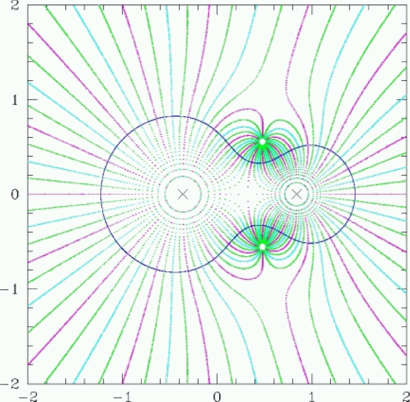
Figure 1: The field lines emanating from the lens positions marked by X flow into the limit points and infinity. The mass fraction of the smaller mass on the right is $\epsilon_{2}=0.3$, and the same number of field lines emerge from each lens position. The field lines from the dominant mass sweep the larger part of the lens plane. The closed curve is the critical curve and is orthogonal to the field lines. Three bifurcation points can be seen: one on the lens axis and two off the axis.

then $\varphi$ changes by $\pi$ around each (finite) limit point, $2\pi$ around the infinity, and $-2\pi$ around each lens position where the positive orientation is counterclockwise as usual. So, the phase angle of $\kappa$ defines the stream lines or field lines that flow from the lens positions to the finite limit points and infinity. See figure 1 for the field lines of a binary lens. The magnitude $|\kappa|$ behaves as the potential and decreases monotonically along the field lines from $|\kappa|=\infty$ at the lens positions to $|\kappa|=0$ at the limit points. The equipotential curves ($|\kappa|=$ constant) are smooth because the lens equation is smooth everywhere except at the poles ($\kappa=\infty$) and are orthogonal to the field lines ($\varphi=$ constant). The total number of field lines that cross an arbitrary equipotential curve ($|\kappa|=$ constant) which may consist of multiple loops is $\Delta\varphi=2\pi n$.

The Critical Curve is but an Equipotential Curve given by $|\kappa|=1$.   The critical curve is an equipotential curve (with the potential value $1$) since $|\kappa|=1$ where $J=0$, and it is easy to visualize the configurations because of the orderly behavior of the family of equipotential curves. If we consider the lens plane as a large two-sphere (with one point $\infty$ at infinity – the well-known notion of one-point compactification), the equipotential curves and field lines can be considered latitudes and longitudes of a multiple-pole sphere with the north poles at the lens positions (“sources”) and the south poles at the limit points and infinity (“sinks”). Check the critical curves in this paper for the predictable configurations. The normals to the equipotential curves and field lines form a right-handed basis vector field.

$$\{\nabla|\kappa|,\nabla\varphi\}\Leftrightarrow 2\{\bar{\partial}|\kappa|,\bar{\partial}\varphi\}$$ (10)

The multiplicity of the “sources” and “sinks” implies that there are “forks” in the streamlines where the equipotential curves bifurcate. The bifurcation points (or saddle points:  $\partial\kappa=0$) are four-prong vertices (or $\times$-points), and the basis vectors are not uniquely defined at the bifurcation points. There are three bifurcation points in every binary lens (Rhie, 2001). For higher $n$ ($>2$), the number varies with the lens parameters.

A critical loop (a connected closed curve with $J=0$) can be assigned an integer or a half-integer because of the analyticity of $\kappa$. If the closed curve encloses $N_{\times}$ lens positions and $N_{\ast}$ limits points, we define the associated topological charge $e$ as follows. (It is valid for an arbitrary closed curve that is analytically connected to the critical curve: the residue theorem.)

$$e=N_{\times}-{N_{\ast}\over 2}$$ (11)

Then the net flux of the field lines that flow out through the critical loop is $\Delta\varphi=2\pi e$. The charge of a limit point is negative ($e=-1/2$) because the field lines flow in while the charge of a lens position is positive ($e=1$). The relative sign reflects the opposite orientations of the critical loops around a limit point and a lens position, which derives from the analytic behavior of $\kappa$ around a zero and a pole in equations (7) and (6). The critical curve of a lens can consist of many loops, and the topological charges associated with the critical loops are subject to a constraint because the total number of field lines is determined by the number of lens elements $n$:  $\Delta\varphi=2\pi n$.

$$\sum_{j}|e_{j}|=n$$ (12)

If $z$ is a Critical Point, $\omega(z)$ is called a Caustic Point.   Since the lens equation is smooth (and so continuous) in the neighborhood of the critical curve, the caustic curve  $\{w(z)|\ |\kappa(z)|=1\}$ shares the connectivity of the critical curve and is smooth except at the stationary points where cusps form. The caustic curve is made of the same number of loops the critical curve is made of and bifurcates where the critical curve bifurcates. So a caustic loop is associated with the same topological charge of the corresponding critical loop, and we will see that the charge $|e|$ measures the smooth rotation of the tangent of the caustic loop. At the cusps, the tangents change the directions abruptly by $\pi$. The critical points that are mapped to cusps under the lens equation are called precusps.

In the case of a single lens (Schwarzschild lens), every point on the critical curve (Einstein ring) is a precusp, and the point caustic may be considered a degenerate cusp. If we look at the caustics in this paper, the cusps are just a finite number of punctuations on the otherwise smooth curves. So our guiding thought for an intuitive or impressionistic understanding (or handwaving) would be: How badly are the critical curves of $n$-point lenses deviated from the circular Einstein ring of a single lens? If we look at the critical curves in this paper, we do find some comforting similarities in the segments around lens positions. That is where the critical curve is more or less tangential to the critical direction ($E_{-}$ defined below). The segments around limit points include parts where the critical curve is more or less normal to the critical direction. If we look at the critical curve in figure LABEL:fig_idomain, its (extrinsic) curvature sign changes around the precusps corresponding to the off-the-axis cusps, but $E_{-}=ie^{-i\varphi}$ smoothly rotates with increasing $\varphi$ along the critical curve. So, it should not be surprising that the connected critical curve behaves differently around the limit points from around the lens positions.

The critical condition $J=0$ implies that (at least) one of the eigenvalues of the Jacobian matrix ${\cal J}$ vanishes on the critical curve. The $2\times 2$ matrix ${\cal J}$ has two eigenvalues , and $\lambda_{-}$ vanishes on the critical curve.

$$\lambda_{\pm}=1\pm|\kappa|$$ (13)

The eigenvectors ($\pm e_{\pm}$: blind to the senses) are conveniently described by the basis vectors ($e_{\pm}$) (with definite orientations).

$$e_{+}\equiv{e^{-i\varphi}\choose e^{i\varphi}}\ ,\quad e_{-}\equiv{i~{}e^{-i\varphi}\choose-i~{}e^{i\varphi}}\ ;\qquad||e_{\pm}||=\sqrt{2}$$ (14)

An arbitrary vector $dz$ can be decomposed in terms of the basis vectors: $dz=dz_{+}E_{+}+dz_{-}E_{-}$ where $dz_{\pm}$ are real and $E_{\pm}$ denote the upper components of $e_{\pm}$.

The Critical Direction is $\pm E_{-}$. The Caustic Curve is Tangent to $\pm E_{+}$.   Let $dz$ be an arbitrary displacement from a critical point $z_{c}$, then $\lambda_{-}(z_{c})=0$, and $d\omega=dz_{+}\lambda_{+}E_{+}=2dz_{+}E_{+}$. So the lens equation is critical or stationary in the eigendirection $\pm E_{-}$:  if $dz_{+}=0$, then $d\omega=0$. If $dz=dz_{-}E_{-}$, the lens equation restricted to the critical direction is quadratic (Rhie and Bennett, 2000).

$$\delta\omega_{2c}={1\over 2}\bar{\partial}J~{}dz_{-}^{2}={1\over 4}~{}dz_{-}^{2}~{}\left(\partial_{+}JE_{+}+\partial_{-}JE_{-}\right)\ ,$$ (15)

where $dJ=dz_{+}\partial_{+}J+dz_{-}\partial_{-}J$. In an exact analogy to the real function $y=x^{2}$ we discussed above, the equation (15) has two solutions ($\pm dz_{-}$) only if $\delta\omega_{2c}/\bar{\partial}J>0$. Then, the remaining question is: Where is $\bar{\partial}J$ pointing? In the $z$-plane, it is a normal vector to the critical curve (or any equipotential curve): it is normal outward to the critical curve with positive topological charge $e>0$, and normal inward to the one with $e<0$. In order to determine the relative direction of $\bar{\partial}J$ in the neighborhood of the caustic curve (in the $\omega$-plane), we need to find a reference direction that is well defined intrinsically. We first note that the caustic curve is always tangent to the eigendirection $\pm E_{+}$. So the normal component $(\partial_{-}JE_{-})$ determines on which side of the caustic curve a point source at $\omega(z_{c})+\delta\omega_{2c}$ produces two images at $z_{c}\pm dz_{-}$ and we can use the (extrinsic) curvature vector of the caustic curve as the reference direction.

If $dz=dt$ is tangent to the critical curve ($d\varphi>0$), $d\omega(z)$ is tangent to the causic curve and is in the direction of $(\partial_{-}JE_{+})$.

$$\delta\omega_{1}=2dt_{+}E_{+}={|dt|\over|\bar{\partial}J|}~{}\partial_{-}JE_{+}$$ (16)

The second order term shows that the caustic curve bends in the direction of $(-\partial_{-}JE_{-})$.

$$\delta\omega_{2t}={1\over 2}\bar{\partial}\bar{\kappa}~{}dt^{2}={1\over 4}|dt|^{2}~{}(\partial_{+}JE_{+}-\partial_{-}JE_{-})$$ (17)

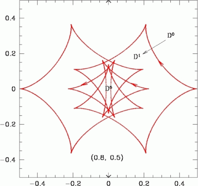
Figure 2: Four point masses are at $x_{1,3}=\pm 0.8$ and $x_{2,4}=\pm 0.5i$. The caustic curve consists of three caustic loops: $(q,m)=(3,12),(1,3),(1,3)$. The arrows show the orientation of the caustic loops ($d\varphi>0$). $D^{0}$ is the lowest degree domain where the number of images is 5, and the domain $D^{1}$ generates 7 images. $D^{0}\longrightarrow D^{1}$ depicts the direction in which the number of images increases by two in relation to the orientation of the caustic loop. All the caustic loops wind around in the same direction – counterclockwise. Crossing through an intersection point changes the degree of caustic domain by two and the number of images by four. In this lens configuration, there are no intersection ponts where more two curves intersect. A point source in $D^{5}$ generates 15 images.

So, if $\pm E_{+}$ define the $x$-axis such that the caustic curve is convex upward, then the quadratic equation (15) has two solutions where $y\equiv\delta\omega_{2c}>0$ and none where $y<0$. We also observe from (16) and (17) that the tangent to the caustic curve rotates clockwise ($d\varphi>0$) unless $\partial_{-}J=0$. See figure 2 for an illustration. So, in order to form a caustic domain that produces many images, the caustic curve will have to wind around many times (here always counterclockiwise) intersecting itself and nesting. The caustic curve in figure 2 has total winding number 5.

The lens equation restricted to the critical curve is stationary ($\delta\omega_{1}=0$) where $\partial_{-}J=0$, and the caustic curve develops a cusp. If $m$ is the number of the cusps of a caustic loop, the tangent of the caustic loop rotates by $-2\pi|e|$ (clockwise) in total on the smooth segments and flips by $m\pi$ at the cusps resulting in the net rotation of $2\pi q=m\pi-2\pi|e|$ where $q$ is the winding number.

$$q={m\over 2}-|e|$$ (18)

A caustic loop with $q\geq 2$ intersects itself and can form a caustic domain where a point source generates $2q$ more images than outside the caustic loop. $|e|$ is easily determined from the corresponding critical loop and subject to the constraint $\sum_{j}|e_{j}|=n$ in equation (12). Caustic loops intersect and nest each other, and the number of images jumps by two at each crossing of the caustic loop. The case $q=1$ is like an $m$-gon (polygon with $m$ vertices) and $|e|$ amounts to the total internal angle in units of $2\pi$. A critical loop enclosing a limit point has $|e|=1/2$, and so the corresponding caustic loop has “internal angle” $\pi$ and is triangular: $(q,m)=(1,3)$. The caustic curve of a quadruple lens in figure 2 consists of two triangular caustics and one with 12 cusps: $(q,m)=(3,12)$, and it satisfies the constraint $\sum_{j}|e_{j}|=1/2+1/2+3=4$.

A corollary will be the theorem of even number of cusps (SEF, pp213). From equations (18) and (12),

$$\sum_{j}{m_{j}\over 2}=n+\sum_{j}q_{j}\ .$$ (19)

Since the RHS is an integer, $\sum_{j}m_{j}$ is an even number. Thus in an $n$-point lens, the number of caustic loops with odd number of cusps is always even. In a binary, trioids: $(q,m)=(1,3)$ appear in a pair that are reflection symmetric with respect to the lens axis. The triple lens in figure 1 in Rhie (1997) consists of two caustic loops with odd number of cusps: $(q,m)=(1,3)$ and $(2,9)$. The quadruple lens in figure 2 includes two trioids.

3 Can a Quadruple Lens Produce 17 Images?

The fact that there are triple lenses that can produce up to 10 images was discovered while we were investigating the location of a point source that produces images at the limit points (Rhie, 1997). There are four (finite) limit points in a triple lens, and the number of images of the point source that produces images at the four limit points must be at least ten because there are always two more negative images than positive images. Since a triple lens can produce no more than 10 images, a correlation between the maximum possible number of images and the limit points was suspected. We found that a point source can produce an image at each of $2(n-1)$ limit points only in the cases of $n=2$ and $n=3$.

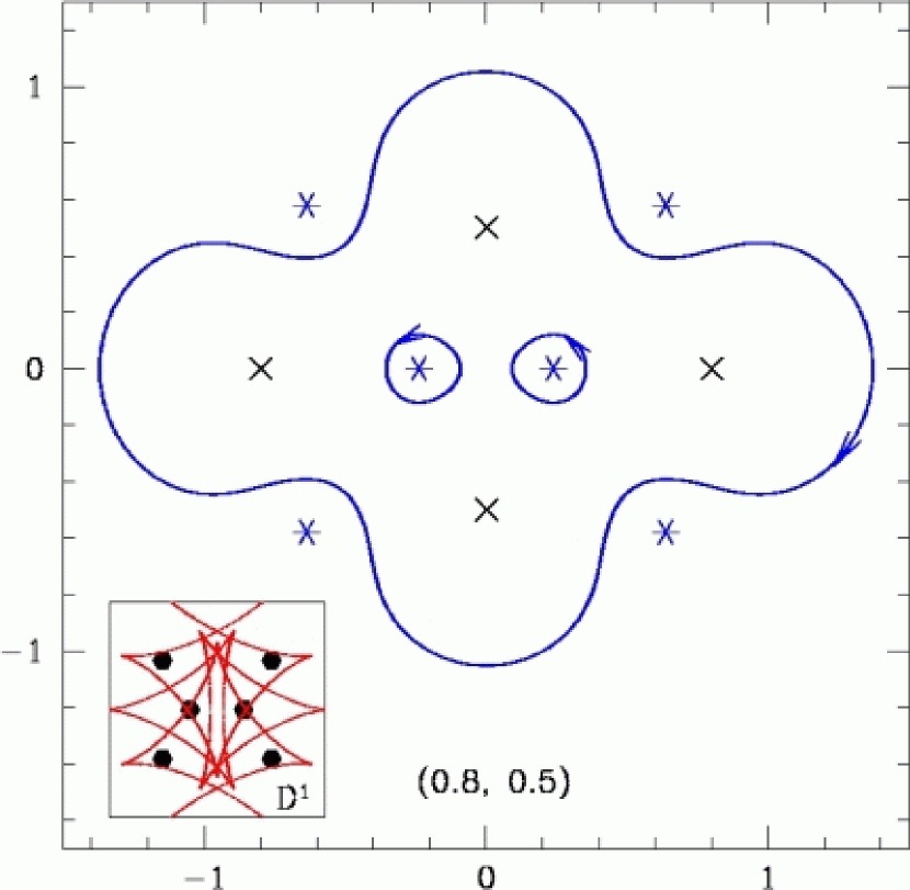
Figure 3: The critical curve for the lens in figure 2 consists of one large loop with $e=3$ and two small loops each with $e=-1/2$. The 6 finite limit points ($z_{\ast}$) are marked by $\ast$’s, and their corresponding positions ($\omega_{\ast}$) in the $\omega$-plane are shown in relation to the caustic curve in the inset. None of the limit points are the image positions of a source in the domain $D^{5}$.

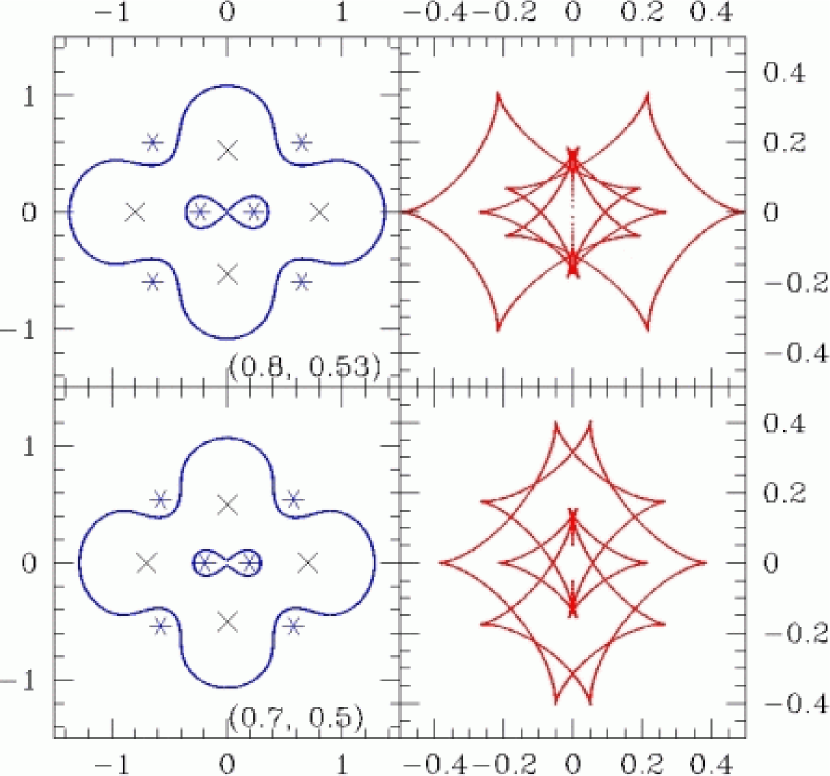
Figure 7: The rhombus lens configuration in figure 2 and figure 3 is changed so that the rhombus becomes more regular. The shorter diagonal is extended in the upper panel and the longer diagonal is shortened in the lower panel. The two critical loops around the limit points at the center merge into one, the corresponding caustic loops merge, and the caustic domains ${\cal D}^{5}$ shrink into the small areas defined by the 8-cusp caustic loops. The 8-cusp caustics unwrinkle into 4-cusp caustics as the rhombus becomes more regular.

If a quadruple lens were to produce 17 images with all the positive images at the limit points, there would have to be 7 limit points because there are always three more negative images in a quadruple lens. A quadruple lens has only 6 (finite) limit points. We find quadruple lenses with 6 distinct (or non-degenerate) limit points that can have caustic domains ${\cal D}^{5}$ where a source produces 15 images (Fig. 2, Fig. 7), and the limit points ($z_{\ast}$) are not mapped onto one point in the $\omega$-plane (Fig. 3). We can see from figure 2 and figure 3 that one extra limit point and associated $|e|=1/2$ caustic curve could make a domain ${\cal D}^{6}$ with 17 images, but that would violate the constraint $\sum_{j}|e_{j}|=4$ (and the theorem of even number of cusps).

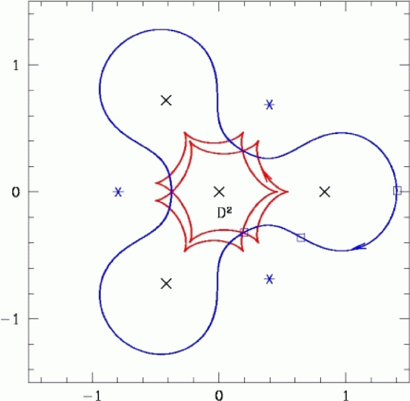
Figure 4: The highly symmetric triple-like quadruple lens has only 3 distinct limit points because each one is doubly degenerate. Three precusps are marked by open squares, and the other nine can be easily identified from the three through the symmetry. The three precusps near the center are notable because they reflect the equal strengths of the topological charges of the degenerate limit points ($e=-1$) and the lens positions ($e=1$). The critical can be considered to consist of six segments each of which is concave toward one of the three lens posistions off the center or one of the three limit points and marked by three precusps.

The quadruple lens in figure 4 is triple-like and allows a source position that has an image at every limit point. The limit points are (doubly) degenerate due to the high degree of symmetry of the lens configuration, and the caustic curve is relatively simple accommodating only up to ${\cal D}^{2}$ where a source generates 9 images (3 positive images and 6 negative images); a source at the center produces 3 images on each three-fold symmetry axis. If the three lens elements off the center are on a circle of radius $a$, the 3 positive images of the source at the center are formed at the limit points when $a=2^{-{1\over 6}}=0.89$.

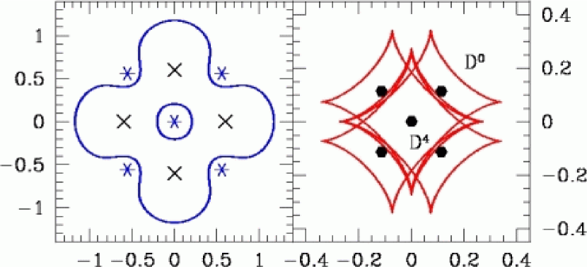
Figure 5: Four equal mass lens elements are equally spaced on a circle of radius $a=0.6$. The four-fold symmetry forces the limit point at the center to be degenerate. The small critical loop at the center has $e=-1$, and the corresponding caustic loop with four cusps can be seen on the right panel. Each lens position claims a segment of the large critical loop each with three precusps. The caustic curve with $|e|=3$ has total 12 cusps, and four of them are hard to distinguish from the four cusps of the caustic loop $|e|=1$. The highest degree caustic domain is ${\cal D}^{4}$ where a point source generates 13 images. When $a=3^{1\over 4}/2=0.658$, a point source at the center of mass generates 5 positive images at the limit points.

The quadruple lens in figure 5 has five distinct limit points because the one at the center is doubly degenerate, and the highest degree caustic domain is ${\cal D}^{4}$ where a source generates 13 images. As the two limit points at the center in figure 3 merges, the two intersecting triangular caustics in figure 2 “merge and unwrinkle” into a quadratic caustic in figure 5. An intermediate step after the “merger” is shown for two cases in figure 7: the domains ${\cal D}^{5}$ are split and diminished in size. If we consider a family of lenses in which four equal mass lens elements are equally spaced on a circle of radius $a$ (such that $x_{1}=a$), the source at the center of mass generates 5 positive images at the limit points when $a=3^{1\over 4}/2=0.658$. The total number of images is 13, and the source is in ${\cal D}^{4}$ which is the highest degree caustic domain for the family of regular rhombus lens configurations.

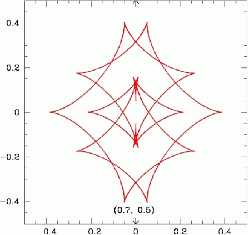
Figure 8: The curves have $e=4$. The critical curve is almost pinching off a critical loop around a limit point ($z_{\ast}$), and the caustic curve shows a triangular shape segment enclosing the corresponding point $\omega_{a}st$. The little sharp “wrinkles” around the opening of the triangle are common in $n$-point lenses with $n\geq 3$ because the caustic curve intersects itself.

What is implied is that the maximum number of images can be obatined when the configuration of the lens elements is largely symmetric to maximize the gravitational interference of all the lens elements as a whole but not so symmetric as to generate degenerate limit points. When the lens elements are dispersed, the gravitational interference is fractionized and the lens system effectively behaves like a linear sum of lower number of lens systems (Fig. 8). When the limit points are degenerate, each degeneracy costs 2 images. In fact, the limit points do not have to be degenerate to cost images: When they are close enough, the critical loops around two limit points merge to form one connected positive image domain. The residual highest degree domains ${\cal D}^{5}$ in figure 7 disappear quickly when the lens configurations become more regular. One trivial nontheless worthy point to note is that a degenerate limit point can host only one image of a point source (property of the lens equation) even though the degeneracy has its direct bearing on the $e$-charge of a loop (such as critical loop) enclosing it (linear differential behavior of the lens equation). Then, the significance of the limit points must lie in that they are the “markers” of positive image domains, which we will conjecture to be the case after briefly examining the notion of image domains.

The Images of the Caustic Curve Defines the Image Domains.   We are convinced by now that the caustic curve of a lens defines the caustic domains, and it is clear what we must have meant by the fact that the caustic domain ${\cal D}^{5}$ of the quadruple lens in figure 2 generates 15 images. There are 15 image domains in the image plane whose boundaries are mapped onto the boundary of the ${\cal D}^{5}$ under the lens equation. The image plane with the domain boundaries of the quadruple lens is a bit of mess to use for an illustration even though we can say that it is rather pretty. So, let’s examine the class of binary lenses that offers a simple laboratory case for the notion of image domains; the caustic curves are simple curves (winding number $q=1$) and there are only two types of caustic domains: outside for 3 images and inside for 5 images. The fact that the caustic curve is sandwiched between the domains of 3 images and 5 images implies that the caustic curve itself generates 4 images. In other words, there are 4 curves in the image plane that are mapped onto the caustic curve, one of which is obviously the critical curve. The critical curve is smooth as we are all familiar with by now, but the others do have cuspy points. The lens equation at the cuspy points is smooth without criticality, and so the corresponding cusps (kinky points) on the caustic curve generate kinky points in the $z$-plane.

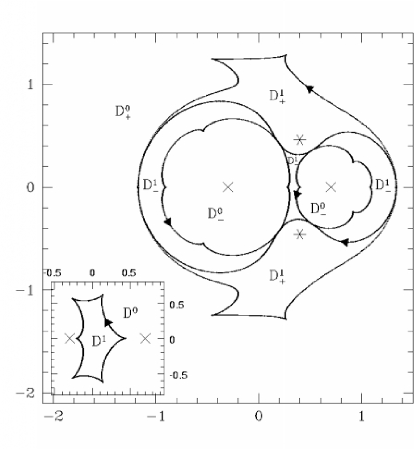
Figure 9: Image domains of a binary lens caustic with six cusps. The arrows indicate the orientations of the caustic curve (inset), the image curves of the caustic curve. The positions of the triangle arrows are the source and image positions and one can infer the speeds of the image motions along the critical curve and precaustic curves. The smooth curve is the critical curve. When the source is outside the caustic curve (${\cal D}^{0}$), there are 3 images (2 ${\cal D}^{0}_{-}$ and 1 ${\cal D}^{0}_{+}$). A source inside the caustic curve (${\cal D}^{1}$) generates 5 images (3 ${\cal D}^{1}_{-}$ and 2 ${\cal D}^{1}_{+}$). Each domain ${\cal D}^{1}_{+}$ is associated with one finite limit point. The positive domain ${\cal D}^{0}_{+}$ is associated with the limit point at $\infty$.

Figure 9 shows the image domains of a binary lens with a connected caustic with six cusps that are defined by the 4 images curves of the caustic curve shown in the inset. Smooth one is the critical curve, and the other 3 curves are tangent to the critical curve at the precusps (each curve is attached to the critical curve at two precusps). The 3 curves are smooth at the precusps on the critical curve where the lens equation (restricted to the critical curve) is stationary, hence each of the 3 curves have four cuspy points that are the images of the cusps of the caustic curve where the lens equation is non-critical. The four curves that are the image curves of the caustic curve form 5 image domains around the critical curve. They are where the 5 images of an emission source inside the caustic curve form and consist of 3 negative image domains (labelled ${\cal D}^{1}_{-}$) and 2 positive image domains (${\cal D}^{1}_{+}$). The limit points are marked by $\ast$ as is the case throughout this paper, and they are inside the two positive domains ${\cal D}^{1}_{+}$. The entire lens plane is divided into 8 domains by the image curves of the caustic curve: $5\ {\cal D}^{1}$’s and $3\ {\cal D}^{0}$’s, and they account for 3 images for a source outside the caustic curve and 5 images for one inside. If we consider our Local Group as a binary lens made of the Galaxy and M31 at a cosmological distance, an elliptical source galaxy can fill the inside caustic domain to produce a large ring image with two holes which we may refer to as “thick Einstein ring” with two holes.

In the neighborhood of a precusp the image domains are divided into four sections, which is related to the fact that the lens equation restricted to the critical direction is cubic at a precusp and produces 3 solutions when the source is inside the caustic and 1 solution when the source is outside. The four domains around a precusp consist either of 3 positive image domains and 1 negative image domain (say, type $+$), or of 1 positive image domain and 3 negative image domains (type $-$). The two cusps on the lens axis are of type $+$, and the four cusps off the lens axis are of type $-$. When a source crosses the caustic through a cusp of type $+$  ($-$), two positive (negative) images are created and move in a tangential direction to the critical curve, and one positive (negative) image crosses the critical curve changing its parity. The net parity remains the same as it does when the caustic crossing is away from a cusp. It should be worth reemphasizing that the well-known statement that two images of opposite parities appear or disappear at a caustic crossing which is strictly valid for line caustic crossings has to be relaxed for cusp crossings because the pair of images that appear or disappear have the same parities (rh97).

These microscopic discussions which may seem irrelevant or annoyingly nitpicking fit together rather naturally once we draw the image domains, and simple intuitive interpretations fall out: A source near a cusp inside the caustic has 3 highly magnified images because they are all near the critical curve; if the source moves along a line caustic, two images remain large because they are near the critical curve and the 3rd one shrinks because it is away from the critical curve; the 3rd image did not come into the picture as the other two small images when we considered the quadratic equation for two large images in equation (15) because of its distance from the critical curve. The mysterious behavior of the parities of the two images that appear or disapper across the caustic curve we discussed above (and once was a source of caustic comments from referees) is just a partner swapping process among the three highly magnified images whose process one can comprehend easily by considering a source moving along the caustic curve past a cusp; the caustic curve near a cusp is reflection-symmetric with respect to its tangent vector (eigenvector $E_{+}$) at the cusp, and a source approaching the cusp along the symmetry axis from inside the caustic generates two images that are reflection-symmetric with respect to the symmetry axis and one image on the symmetry axis; the two images off the symmetry axis ($E_{+}$) are on the same side of the critical curve and so have the parity.

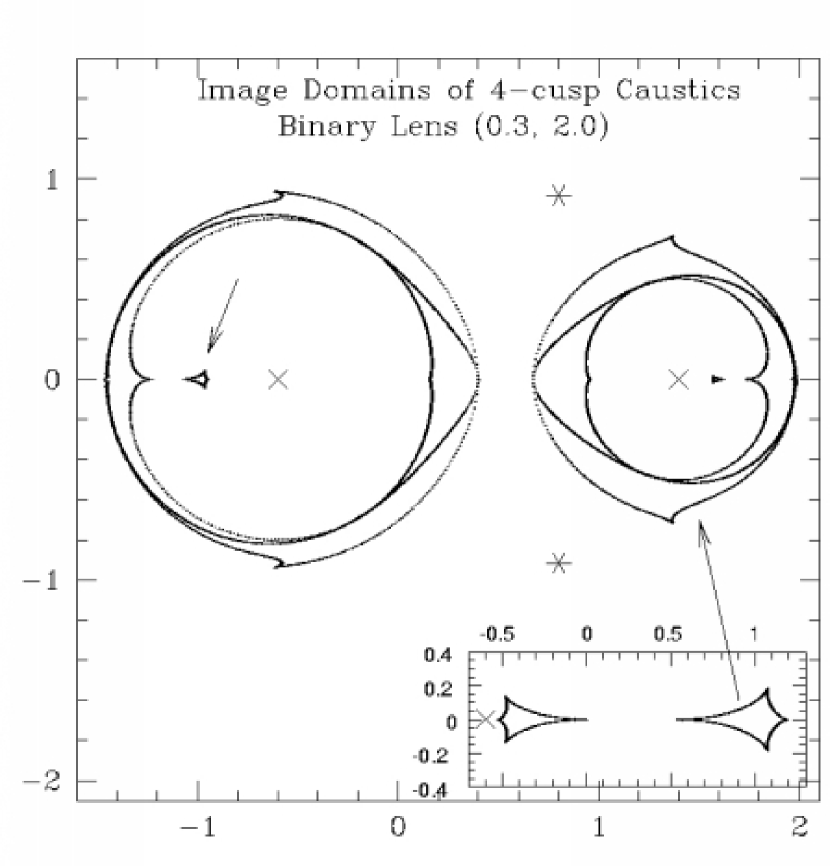
Figure 10: Image domains of a binary lens caustic with four cusps. The interior of each quadroid commands 5 image domains. The “thick Einstein rings” (image rings) are made of 4 image domains (2 positive and 2 negative) as indicated by the long arrow. The fifth image in the small (negative) image domain indicated by the short arrow has a high probability to be missing in an observation. The smooth curve is the critical curve. Despite the oval shapes of the critical loops, the “thick Einstein rings” are more or less circular annuluses. The Einstein ring of each lens element as a single lens traces more or less the middle of the corresponding image ring as centered at the lens position ($\times$).

Figure 10 shows the image domains of a case where the caustic curve with six cusps is split into two quadroids. The long arrow indicates 3 large image curves of the 4-cupsed caustic centered around $(0,1)$. If a quasar with its host galaxy covers this caustic loop, there will be four images of the quasar and the finite size galaxy will form a ring image with one hole. Two of them are postive images and the other two are negative images. The fourth image curve of the caustic is inside the the image ring of the other caustic loop and is marked by the shorter arrow. This small image domain generates the fifth image (negative image) and has a high probability to become a missing image because of its smallness. What we note is that when the critical curve splits, the number of positive image domains for each caustic loop is never more than the number of positive image domains of the connected caustic curve which is the same as the number of the finite limit points.

In the case of lensing by an elliptical projected mass distribution (zeroth approximation of a galaxy lens), the caustic consists of one quadroid (or astroid), and the fifth image of a quasar lensed by a galaxy is more likely to be missing due to the brightness of the sizeable lensing galaxy. However, the color difference of the lensing galaxy and the lensed quasar may reveal the small fifth image in high resolution images. The position of the fifth image in relation to the image ring will be one of the clinching constraints in the reconstruction of the image domains and so the lens characteristics. Draw a circle of radius $\sqrt{0.3}=0.548$ centered at the lens position (marked $\times$) of the smaller “thick Einstein ring” (arrowed) in figure 10 and note that the circle goes through just about the middle of the image ring donut. The circle is the Einstein ring of the lensing mass $0.3$ as a single lens. Thus, one can more or less read off the lensing mass from the image ring. The apprearance of the observed image ring of a host galaxy of a quasar depends on the position of the source with respect to the caustic, of course, but the distribution of the bright core images of the quasar offers information on the point source position. We will discuss the image domains, “thick Einstein rings”, and Einstein rings of extended mass distribution lenses elsewhere (Rhie, 2001).

4 A Conjecture on the Number of Images

We have meandered through the properties of the caustic curve, the image curves of the caustic curve, image domains, the critical curve and smoothly rotating Jacobian eigenvectors on the critical curve, and the limit points and lens positions as the “sinks” and “sources” of the potential defined by $|\kappa(z)|$. The number of images jumps across the caustic curve because of the pairs of positive and negative images across the critical curve. Thus, if we refer to the image curves of the caustic curve other than the critical curve as precaustic curves, the critical curve is “padded” from both sides by the positive and negative image domains defined by the precaustic curves. Precaustic curves are tangentially attached to the critical curve at designated precusps, and their $J$ values are either positive (positive precaustic curve) or negative (negative precaustic curve) except at the precusps where they are tangent to the critical curve. The number of positive images of a given caustic is given by the number of positive image domains that are mapped to the caustic domain by the lens equation, and figure 9 and 10 illustrate that each positive image domain defined by a positive precaustic curve is associated with a finite limit point. So, a conjecture follows.

1. Conjecture:  The number of positive images of an $n$-point lens is bounded by the number of finite limit points $2(n-1)$ for $n>1$. When $n=1$, there is one limit point at $\infty$ and a point source has one positive image as is well known.

2. Corollary:  The total number of images of an $n$-point lens can not exceed $5(n-1)$ when $n>1$. When $n=1$, there are two images.

3. The maximum number of images of an $n$-point lens can not be less than $3(n+1):n\geq 3$.

The corollary follows from the conjecture because there are always $(n-1)$ more negative images in an $n$-point lens. In order to prove the third item, we consider a lens consisting of $n$ equal masses equally spaced on a circle of radius $a$ can produce an image at every distinct limit point. We choose a source at the center of circle to maximally utilize the symmetry and examine the cases of $n=2^{k}$. The lens equation (1) becomes as follows where $z_{j}\equiv z-x_{j}$.

$$z=\sum_{1}^{n}{1\over n}{1\over\bar{z}_{j}}\equiv\bar{F}_{n}$$ (20)

For $n=2$, we let $x_{1,2}=\pm a$, and

$$\bar{F}_{2}={\bar{z}\over\bar{z}^{2}-a^{2}}\ .$$ (21)

For $n=4$, we add two equal masses at $x_{3,4}=\pm ia$, and

$$\bar{F}_{4}=\bar{F}_{2}(a^{2})+\bar{F}_{2}(-a^{2})={\bar{z}^{3}\over\bar{z}^{4}-a^{4}}\ .$$ (22)

The pattern is clear: $\bar{F}_{8}=\bar{F}_{4}(a^{4})+\bar{F}_{4}(-a^{4})$, etc, and

$$\bar{F}_{n}=={\bar{z}^{n-1}\over\bar{z}^{n}-a^{n}}\ .$$ (23)

The limit points $z_{\ast}$ are the zeros of $\partial F_{n}$.

$$0=z^{n-2}(z^{2}+(n-1)a^{n})$$ (24)

The center $z_{\ast}=0$ is an (n-2)-th order zero and satifies the lens equation (and so an image). Other $n$ zeros are on the circle of radius $r_{\ast}=(n-1)^{1/n}a:r_{\ast}<a$.

$$z_{\ast}=r_{\ast}e^{\pi\over n},\ r_{\ast}e^{3\pi\over n},\ ...\ r_{\ast}e^{(n-1)\pi\over n}$$ (25)

They are images when $a=a_{n}$.

$$a_{n}=n^{-{1\over 2}}(n-1)^{n-2\over n}$$ (26)

As $n$ becomes large, $a_{n}$ converges to $1$. Since the $n$-point “necklace” lens has $(n+1)$ distinct limit points, the source at the center produces no less than $(n+1)$ positive images, or equivalently no less than $3n+1$ images in total. One image is at the center, and $3n$ images are on three circles of radius $r_{\ast}$ ($n$ positive images), $r_{<}<a$ ($n$ negative images), and $r_{>}>a$ ($n$ negative images). In the case of $n=4$, $a=0.658$, $r_{\ast}=\sqrt{3}/2=0.866$, $r_{<}=0.5$, and $r_{>}=1/2+\sqrt{7}/4=1.16$. We have analysed the cases where $n$ is power of 2, but the (discrete) axial symmetry of the “necklace” lenses gurantees that $3n+1$ is the lower bound of the maximum total number of images of arbitrary $n$-point lenses.

The formula $3n+1$ produces the correct maximum possible number of images $10$ for $n=3$ because it happens to be that the two formulae for the number of limit points $2(n-1)$ and $n+1$ coincide when $n=3$. Mao et al. (1997) numerically examined some cases of the family of “necklace” lenses and observed that the maximum number of images was $3n+1$. The formula $3n+1$ predicts too many images for $n=2$ and $n=1$ because the number of the limit points is less than $(n+1)$ and 2 less images for $n=4$. Here we have shown that $3n+1$ is the lower bound of the maximum possible number of images of an $n$-point lens for $n\geq 3$ by investigating source positions that generate positive images at the limit points as we did in rh97.

Figure 6: As the lens separation increases, the gravitational interference is fractionized and the “traffic” of the caustic curves in the central region moves in the way the highest degree domain in the center shrinks. ${\cal D}^{4}$ disappears at $a=1/\sqrt{2}$, and the central region becomes ${\cal D}^{0}$ where the number of images is the minimum 5. With increasing $a$ ($x_{1,3}=\pm a,\ x_{2,4}=\pm ia$), the caustic curve degenerates into caustic loops directly associated with the lens elements and the loops shrink and unwrinkle.

References

- Alcock (2000) Alcock, C. 2000, Science, 287, 74
- Bennett et al. (2000) Bennett, D., Rhie, S. H., Becker, A. C., Butler, N., Dann, J., Kaspi, S., Leibowitz, E., Lipkin, Y., Maoz, D., Mendelson, H., Peterson, B., Quinn, J., Shemmer, O., Thomson, S., and Turner, S. E. 1999 Nature, 402, 57
- Bennett and Rhie (2000) Bennett, D., and Rhie, S. H. 2000, ApJ, submitted (astro-ph/0011084)
- Bennett and Rhie (2001) Bennett, D., and Rhie, S. H. 2001, Multiple Planetary Systems as Gravitational Triple Lenses
- Broadhurst et al. (2000) Broadhurst, T., Huang, X., Frye, B., and Ellis, R. 2000, ApJ, 534, 15
- Burke (1981) Burke, W. 1981, ApJ, 244, 1
- Gil-Merino et al. (2000) Gil-Merino, R., Goicoechea, L., Serra-Ricart, M., Oscoz, A., Alcalde, D., and Mediavilla, E. 2000, MNRAS, in press (astro-ph/0010284)
- Haarsma et al. (1999) Haarsma, D., Hewitt, J., Lehar, J., and Burke, B. 1999, ApJ, 510, 64
- Kaiser (1998) Kaiser, N. 1998, ApJ, 498, 26
- Kochanek et al. (2001) Kochanek, C., Keeton, C., and McLeod, B. 2001, ApJ, 547, 50
- Landau and Lifshitz (1982) Landau, L., and Lifshitz, E. 1982, Fluid Mechanics, Pergamon
- Mao et al. (1997) Mao, S., Petters, A. O., and Witt, H. J. 1997, The Eighth Marcel Grossmann Meeting on General Relativity, Ed. R. Ruffini, World Scientific (Singapore) (astro-ph/970811)
- Ozernoy et al. (2000) Ozernoy, L., Gorkavyi, N., Mather, J., and Taidakova, T. 2000, ApJ, 537, 1470
- Paczynski (1986) Paczynski, B. 1986, ApJ, 304, 1
- Premadi (2001) Premadi, P., Martel, H., Matzner, R., and Futamase, T., 2001, ApJ, in press
- Rhie (1997) Rhie, S. H. (rh97) 1997, ApJ, 484, 63
- Rhie (2001) Rhie, S. H. 2001, Notes on Gravitational Binary Lenses
- Rhie (2001) Rhie, S. H. 2001, Image Domains, Ring Images, and Einstein Rings of Extended Mass Distribution Lenses
- Rhie and Bennett (2000) Rhie, S. H., and Bennett, D. 2000, ApJ, submitted (astro-ph/9912050)
- Robberto et al. (1999) Robberto, M., Beckwith, S., and Herbst, T. 1999, Proceedings of Star Formation 1999, Nagoya, Japan, June 21 - 25, ed. T. Nakamoto, p. 231-232
- Schechter (2000) Schechter, P. 2000, IAU Symposium No. 201: New Cosmological and the Values of the Fundamental Parameters, eds. A.N. Lasenby and A. Wilkinson (astro-ph/0009048)
- Schneider et al. (1992) Schneider, P., Ehlers, J., and Falco, E. (SEF) 1992, Gravitational Lenses, Springer-Verlag
- Tyson et al. (1998) Tyson, J. A., Kochanski, G., and dell’Antonio, I. 1998, ApJ, 498, 107
- Walsh et al. (1979) Walsh, D., Carswell, R., and Weymann, R. 1979, Nature, 279, 381
- Weinberg (1972) Weinberg, S. 1972, Gravitation and Cosmology, John Wiley & Sons
- Witt (1990) Witt, H. J. 1990, å, 236, 311
- Wyithe and Turner (2000) Wyithe, J. and Turner, E. 2000, MNRAS, in press (astro-ph/0008008)
- Young (1981) Young, P. 1981, ApJ, 244, 756