ISOCAM observations of the $\rho$ Ophiuchi cloud: Luminosity and mass functions of the pre-main sequence embedded cluster ^,

We present the results of the first extensive mid-infrared (IR) imaging survey of the $\rho$ Ophiuchi embedded cluster, performed with the ISOCAM camera on board the ISO satellite. The main $\rho$ Ophiuchi molecular cloud L1688, as well as the two secondary clouds L1689N and L1689S, have been completely surveyed for point sources at 6.7 $\mu$m and 14.3 $\mu$m. A total of 425 sources are detected in $\sim 0.7$ deg², including 16 Class I, 123 Class II, and 77 Class III young stellar objects (YSOs). Essentially all of the mid-IR sources coincide with near-IR sources, but a large proportion of them are recognized for the first time as YSOs. Our dual-wavelength survey allows us to identify essentially all the YSOs with IR excess in the embedded cluster down to $F_{\nu}\sim$ 10–15 mJy. It more than doubles the known population of Class II YSOs and represents the most complete census to date of newly formed stars in the $\rho$ Ophiuchi central region. There are, however, reasons to believe that several tens of Class III YSOs remain to be identified below $L_{\star}\sim 0.2\ \mbox{L${}_{\odot}$}$. The mid-IR luminosities of most ($\sim 65$%) Class II objects are consistent with emission from purely passive circumstellar disks. The stellar luminosity function of the complete sample of Class II YSOs is derived with a good accuracy down to $L_{\star}\sim 0.03\ \mbox{L${}_{\odot}$}$. It is basically flat (in logarithmic units) below $L_{\star}\sim 2\ \mbox{L${}_{\odot}$}$, exhibits a possible local maximum at $L_{\star}\sim 1.5\ \mbox{L${}_{\odot}$}$, and sharply falls off at higher luminosities. A modeling of the luminosity function, using available pre-main sequence tracks and plausible star formation histories, allows us to derive the mass distribution of the Class II YSOs which arguably reflects the initial mass function (IMF) of the embedded cluster. After correction for the presence of unresolved binary systems, we estimate that the IMF in $\rho$ Ophiuchi is well described by a two-component power law with a low-mass index of $-0.35\pm 0.25$, a high-mass index of $-1.7$ (to be compared with the Salpeter value of $-1.35$), and a break occurring at $\mbox{$M_{\mathrm{flat}}$}=0.55\pm 0.25\,\mbox{M${}_{\odot}$}$. This IMF is flat with no evidence for a low-mass cutoff down to at least $\sim 0.06\,\mbox{M${}_{\odot}$}$.

1 Introduction

Recent observations suggest that most stars in our Galaxy and other galaxies form in compact clusters. In particular, near-IR imaging surveys of nearby molecular cloud complexes have shown that the star formation activity is typically concentrated within a few rich clusters associated with massive dense cores which constitute only a small fraction of the total gas mass available (e.g. Lada, Strom, & Myers lada93 (1993), Zinnecker, McCaughrean, & Wilking zinnecker (1993)). These embedded clusters comprise various types of young stellar objects (YSOs) – from still collapsing protostars to young main sequence stars – but are usually dominated in number by low-mass pre-main sequence (PMS) stars, i.e., T Tauri stars. Young clusters provide excellent laboratories for studying the formation and early evolution of stars through the observational analysis of large, genetically homogeneous samples of embedded YSOs. Two key characteristics of these young stellar populations are their luminosity distribution and their mass spectrum, which give important observational constraints on the stellar initial mass function (IMF) in the Galaxy. Observations of young embedded clusters can also help us understand possible links between parent cloud properties and the resulting stellar masses. They are however hampered by: (1) dust extinction from the parent cloud which hides most of the newly formed stars at optical wavelengths, (2) the difficulty to recognize the nature of individual sources (e.g. protostars, T Tauri stars, or background sources), (3) the youth (and thus poorly known intrinsic properties) of most cluster members.

Owing to these difficulties, the census of embedded YSOs provided by IRAS and near-IR studies is far from complete even in the nearest clouds (e.g. Wilking, Lada, & Young wly (1989) – hereafter WLY89). Thanks to its high sensitivity and good spatial resolution in the mid-IR, the ISOCAM camera on board ISO (Cesarsky et al. cesarsky (1996); Kessler et al. kessler (1996)) was a powerful tool to achieve more complete surveys for YSOs in all major nearby star-forming regions (see Nordh et al. nordh1 (1996), nordh2 (1998); Olofsson et al. ohk99 (1999); Persi et al. pmo00 (2000)).

The nearby $\rho$ Ophiuchi cloud is one of the most actively studied sites of low-mass star formation. Its central region harbors a rich embedded cluster with about 100 members recognized prior to the present work (e.g. WLY89, Casanova et al. cmfa (1995)). While a dispersed population of optically visible young stars, associated with the Upper-Scorpius OB association, has a typical age of several million years (Myr) (e.g. Preibisch & Zinnecker pz99 (1999)), the central embedded cluster is recognized as one of the youngest clusters known with an estimated age on the order of $\sim$ 0.3–1 Myr (e.g. WLY89, Greene & Meyer gm95 (1995), Luhman & Rieke lr99 (1999)). This young cluster has been extensively studied at wavelengths ranging from the X-ray to the radio band. The satellites Einstein and $ROSAT$ have revealed $\sim 70$ highly variable X-ray sources associated with magnetically-active young stars, including deeply embedded protostellar sources (Montmerle et al. montmerle83 (1983), Casanova et al. cmfa (1995), Grosso et al. grosso (2000)). In the near-IR, the cloud has been deeply surveyed from the ground using large-format arrays (Greene & Young gy (1992), Comerón et al. crbr (1993), Strom et al. sks (1995), Barsony et al. bklt (1997)). Unfortunately, due to difficulties in discriminating between background sources and embedded YSOs without performing time-consuming mid-IR photometry (e.g. Greene et al. gwayl (1994)) or near-IR spectroscopy (e.g. Greene & Lada gl96 (1996); Luhman & Rieke lr99 (1999)), these recent near-IR surveys have only partially increased the number of classified, recognized members. Finally, while only relatively poor angular resolution $IRAS$ data are available so far in the far-IR (e.g. WLY89), deep imaging surveys at an angular resolution of $10-15\arcsec$ or better exist at (sub)millimeter wavelengths (e.g., Motte, André, & Neri man (1998) – hereafter MAN98 –; Wilson et al. wilson99 (1999)).

It is thanks to the illuminating example of the $\rho$ Ophiuchi embedded cluster that the now widely used empirical classification of YSOs was originally introduced. Three IR classes were initially distinguished based on the shapes of the observed spectral energy distributions (SEDs) between $\sim$ 2 $\mu$m and $\sim$ 25–100 $\mu$m (Lada & Wilking lw84 (1984), WLY89). Objects with rising SEDs in this wavelength range were classified as Class I, sources with SEDs broader than blackbodies but decreasing longward of $\sim$ 2 $\mu$m as Class II, and sources with SEDs consistent with (or only slightly broader than) reddened stellar blackbodies as Class III. These morphological SED classes are interpreted in terms of an evolutionary sequence from (evolved) protostars (Class I), to T Tauri stars with optically thick IR circumstellar disks (Class II), to weak T Tauri stars with at most optically thin disks (Class III) (Lada lada87 (1987), Adams, Lada, & Shu als (1987), André & Montmerle am (1994) – hereafter AM94). A fourth class (Class 0) was subsequently introduced by André, Ward-Thompson, & Barsony (awb (1993)) to accommodate the discovery in the radio range of cold sources with large submillimeter to bolometric luminosity ratios and powerful jet-like outflows, such as VLA 1623 in $\rho$ Oph A (e.g. André et al. andre90 (1990); Bontemps et al. batc (1996)). Class 0 objects, which have measured circumstellar envelope masses larger than their inferred central stellar masses, are interpreted as young protostars at the beginning of the main accretion phase (e.g. André, Ward-Thompson, & Barsony awb00 (2000)). The fact that the $\rho$ Ophiuchi central region contains at least two Class 0 protostars (André, Ward-Thompson, & Barsony awb (1993))), as well as numerous ($\lower 2.15277pt\hbox{$\;\buildrel>\over{\sim}\;$}60$) pre-stellar condensations (MAN98), demonstrates that it is still actively forming stars at the present time.

The distance to the $\rho$ Ophiuchi cloud is somewhat uncertain. Usually, a value of 160 pc is adopted (e.g. Chini chini81 (1981)). However, recent Hipparcos results on the Upper-Scorpius OB association (de Zeeuw et al. dezeeuw (1999)) provide a reasonably accurate estimate of $145\pm 2$ pc for the average distance to the stars of the OB association. The embedded cluster is located at the inner edge of the molecular complex on the outskirts of the OB association (e.g. de Geus degeus (1989)), and not very far, in projection, from the association center (less than $4\degr$ apart which corresponds to $\sim 10$ pc; see Fig. 9 of de Zeeuw et al. dezeeuw (1999)). In this paper, we therefore adopt a distance of $d=140\pm 10$ pc for the $\rho$ Ophiuchi IR cluster which corresponds to a distance modulus $5\times$log${}_{10}(d/10\rm pc)=5.73\pm 0.15$.

The layout of the paper is as follows. Sect. 2 gives observational details (§ 2.2) and describes the way the data have been reduced to obtain mid-IR images and extract point-sources (§ 2.3) along with the photometric uncertainties and the sensitivity levels (§ 2.4). In Sect. 3, the identification of detected sources is discussed (§ 3.1) and the selection of a new population of 123 Class II YSOs, as well as 16 Class I and 77 Class III YSOs, is described (§ 3.2-3.5). We then derive luminosities for these YSOs and build the corresponding luminosity functions in Sect. 4. In Sect. 5, we model the luminosity functions for Class II and Class III YSOs in terms of the underlying mass function and star formation history. In Sect. 6, we discuss the resulting constraints on the IMF of the $\rho$ Ophiuchi cloud down to $\sim 0.06\,\mbox{M${}_{\odot}$}$, (§ 6.1-6.2) as well as related implications (§ 6.3-6.5).

2 Observations and data reduction

2.1 Region surveyed by ISOCAM

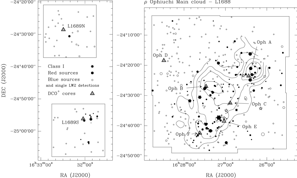
Figure 1: Sky map of the $\rho$ Ophiuchi clouds L1688, L1689N, and L1689S showing the spatial distribution of the ISOCAM sources. The filled symbols correspond to “red” YSOs (i.e. Class I and Class II YSOs, see Sect. 3), while the open circles mark the “blue” sources. The surface areas of these symbols are proportional to the 6.7$\mu$m flux densities. The open stars mark four young early-type stars (SR3, S1, WL22, WL16 from right to left; see Sect. 3.1). The contours show the L1688 molecular cloud as mapped in CS(2-1) by Liseau et al. (1995). The triangles refer to the peaks of the DCO⁺ dense cores of Loren et al. (1990). The figure emphasizes the presence of four sub-clusters Oph A, B, EF (between Oph E and Oph F), and L1689S (named after the associated dense cores).

The survey encompasses the $\rho$ Ophiuchi central region associated with the prominent dark cloud L1688, as well as the two subsidiary sites L1689N and L1689S. The L1688 field is a $\sim 45\arcmin\times 45\arcmin$ square, while the L1689N and L1689S fields each cover an area of $16.5\arcmin\times 16\arcmin$ (see Fig. 1). Most previously known members of the $\rho$ Ophiuchi cluster lie within these fields. In particular, this is the case for 94 of a total of 113 recognized members from WLY89, AM94, Greene et al. (gwayl (1994)), and MAN98. The known young stars which lie outside the boundaries of our survey are mostly optically visible, weak-line or post T Tauri stars (belonging to Class III) spread over a large area on the outskirts of the molecular complex (e.g. Martín et al. martin98 (1998)).

2.2 Observational details

The mapping was performed in the raster mode of ISOCAM in which the mid-IR $32\times 32$ pixel array imaged the sky at consecutive positions along a series of scans parallel to the right-ascension axis. The offset between consecutive array positions along each scan ($\Delta\alpha$) was 15 pixels, while the offset between two scans ($\Delta\delta$) was 26 pixels. Each set of scans was then co-added and combined into a single raster image. The final image of the L1688 field (Fig. 1 and Abergel et al. 1996) actually results from the combination of six separate rasters. A pixel field of view of 6$\arcsec$ was used for four of these rasters, but smaller 3$\arcsec$ pixels were employed for the other two rasters in order to avoid saturating the array on the brightest sources of the cluster. The L1689N and L1689S fields were imaged with one raster each using 6$\arcsec$ pixels.

In order to avoid saturation, the individual readout time for the L1688 rasters was set to $\mbox{$t_{\mathrm{int}}$}=0.28\,$s. About 55 of these readouts (i.e. an integration time of $\sim 15\,$s) were performed per sky position. Thanks to the half-frame overlap between subsequent individual images, each sky position was observed twice, yielding an effective total integration time of $\sim 30\,$s. For L1689N and L1689S it was possible to use $\mbox{$t_{\mathrm{int}}$}=2.1\,$s, and about 15 readouts were performed per sky position with the same half-frame overlap, giving an integration time per sky position of $\sim 60\,$s. A total of 1104 individual images were necessary to mosaic the L1688 field, and an additional 60 images each were used to map L1689N and L1689S.

All three fields were mapped in two broad–band filters of ISOCAM: LW2 (5–8.5 $\mu$m) and LW3 (12–18 $\mu$m). These filters are approximately centered on two minima of the interstellar extinction curve and are situated apart from the silicate absorption bands (at roughly 10 and 18 $\mu$m). However, they include most of the Unidentified Infrared Bands (UIBs, likely due to PAH-like molecules) which constitute a major source of background emission toward star-forming clouds (e.g. Bernard et al. bernard (1993), Boulanger et al. boulanger (1996)). The ISOCAM central wavelengths adopted here for LW2 and LW3 are 6.7 $\mu$m and 14.3 $\mu$m respectively.

2.3 Image processing, source extraction, and photometry

Each raster consists of a temporal series of individual integration frames (i.e. of $32\times 32$ pixel images) which was reduced using the CAM Interactive Analysis software (CIA). We have subtracted the best dark current from the ISOCAM calibration library, and as a second step we improved it with a second order correction using a FFT thresholding method (Starck et al. starck2 (1999)). Cosmic-ray hits were detected and masked using the multi-resolution median transform algorithm (Starck et al. starck1 (1996)). The transients in the time history of each pixel due to detector memory effects were corrected with the inversion method described in Abergel et al. (abergel (1996)). The images were then flat-fielded with a flat image obtained from the observations themselves. Since these various corrections applied to the images are not perfect, the extraction of faint sources from the images is a difficult task. We have developed an interactive IDL point-source detection and photometry program for raster observations which works in the CIA environment. This program helps to discriminate between astronomical sources and remaining low-level glitches or ghosts due to strong transients (see also Nordh et al. nordh1 (1996); Kaas et al. kaas01 (2001)). The fluxes of the detected sources were estimated from the series of flux measurements made in the individual images (usually 2 to 4 individual images cover each source) which were obtained from classical aperture photometry. The emission was integrated in a sky aperture, the background emission subtracted, and finally an appropriate aperture correction was applied based on observed point-spread functions available in the ISOCAM calibration library. In practice, the radius of the aperture used was 9$\arcsec$ (i.e., 3 and 1.5 pixels for a pixel size of $3\arcsec$ and 6$\arcsec$, respectively). For the weakest sources, however, we reduced the aperture radius to 4.5$\arcsec$ (i.e. 1.5 pixels for a pixel size of $3\arcsec$), in order to improve the signal-to-noise ratio. Finally, we applied the following conversion factors: $2.33$ and $1.97$ ADU/gain/s/mJy for LW2 and LW3 respectively (from in-orbit latest calibration - Blommaert blommaert (1998)). These calibration factors are strictly valid only for sources with a flat SED ($F_{\nu}\sim\nu^{-1}$). Here, a small but significant ($\lower 2.15277pt\hbox{$\;\buildrel>\over{\sim}\;$}1$ %) color correction needs to be applied to the bluest sources, recognized as Class III YSOs in Sect. 3 below. For these sources, the conversion factors quoted above were divided by 1.05 for LW2 and 1.02 for LW3 to account for the color effect. The 212 ISOCAM sources recognized as cluster members (see Sect. 3 below) are listed in Table 1 (available only in electronic form at http://cdsweb.u-strasbg.fr/) with their J2000 coordinates, their flux densities and associated rms uncertainties (see Sect. 2.4), as well as the corresponding near-IR identifications.

2.4 Photometric uncertainties and point-source sensitivity

The uncertainties on the final photometric measurements result from systematic errors due to uncertainties in the absolute calibration and the aperture correction factors, and from random errors associated with the flat-fielding noise, the statistical noise in the raw data, the noise due to remaining low-level glitches, and the imperfect correction for the transient behavior of the detectors. The in-orbit absolute calibration has been verified to be correct to within 5 % (Blommaert blommaert (1998)), and we estimate that the maximum systematic error on the aperture correction is $\sim 10\,$% (by comparing theoretical and observed point-spread functions). The maximum systematic error on our photometry is thus $\sim 15\,$%. The magnitudes of the random errors were directly estimated from the data by measuring both a “temporal” noise (noise in the temporal sequence of individual integrations) and a “spatial” noise (due to imperfect flat-fielding and/or spatial structures in the local mid-IR background emission) for each source in the automatic detection procedure. The temporal noise was computed as the standard deviation of the individual aperture measurements divided by the square root of the number of measurements. The spatial noise was estimated as the standard deviation around the mean background (linear combination of the median and the mean of the pixels optimized for the source flux estimates) in the immediate vicinity of each source.

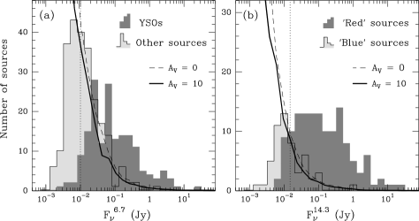
Figure 2: (a) Distribution of the $F_{\nu}^{6.7}$ flux densities for the 425 sources detected by ISOCAM. The dark histogram shows the flux distribution of the cluster members (i.e., YSOs) discussed in Sect. 3, while the light histogram corresponds to the remaining sources which are likely dominated by background Galactic objects. (b) Same as (a) for the $F_{\nu}^{14.3}$ flux densities. The dark histogram shows the flux distribution for the “red” ISOCAM sources (i.e., Class I and II YSOs), while the light histogram comprises only the “blue” ISOCAM sources not associated with recognized YSOs (see Sect. 3 and Fig. 3). The adopted completeness levels equal to 10 and $15\,$mJy for $F_{\nu}^{6.7}$ and $F_{\nu}^{14.3}$ respectively are shown as vertical dotted lines. The solid and dashed curves show the expected number of Galactic sources in each bin according to the model of Wainscoat et al. (1992) for $A_{V}=0$ and $A_{V}=10$ respectively.

The sensitivity limit of the survey was estimated by calculating the average value of the quadratic sum of the temporal and spatial noises measured on the weakest detected sources. The total rms flux uncertainty found in this way, $\sigma_{tot}=(\sigma_{temp}^{2}+\sigma_{spat}^{2})^{1/2}$, is $\mbox{$\sigma_{6.7}$}=2.2$ mJy at 6.7 $\mu$m and $\mbox{$\sigma_{14.3}$}=4.1$ mJy at 14.3 $\mu$m, $\sim$ 75 % of which is due to the spatial noise component. The large contribution of the spatial noise originates in the highly structured diffuse mid-IR emission from the ambient molecular cloud itself (see Abergel et al. abergel (1996)). Figure 2 displays the distributions of fluxes at 6.7 $\mu$m and 14.3 $\mu$m for all the detected ISOCAM sources. We used the Wainscoat et al. (wainscoat (1992)) Galactic model of the mid-IR point source sky to estimate the expected number of foreground and background sources up to a distance of 20 kpc. The model predictions are shown by solid and dashed curves in Fig. 2 for cloud extinctions of $A_{V}=0$ and $A_{V}=10$, respectively (see Kaas et al. kaas01 (2001) for more details). It can be seen that the flux histograms of the ISOCAM sources not associated with YSOs (light shading in Fig. 2) are remarkably similar in shape to the model distributions down to $\sim 6$ mJy at 6.7 $\mu$m and $\sim 10$ mJy at 14.3 $\mu$m. These flux densities can be used to estimate the completeness level of our observations which is not uniform over the spatial extent of the survey. The histograms with light (grey) shading in Fig. 2 are dominated by background sources preferentially located in low-noise regions (i.e., outside the crowded central part of L1688), where the total rms flux uncertainty is $\sim 2.0$ mJy at 6.7 $\mu$m and $\sim 3.5$ mJy at 14.3 $\mu$m. The effective completeness level in these regions is thus $\sim 3\,\sigma_{tot}$, where $\sigma_{tot}$ is the total flux uncertainty (see above). However, most of the YSOs are located in regions where the noise is somewhat larger. The largest rms noise is reached in the Oph A core area (see Fig. 1), where $\sigma_{tot}\approx 3.4\,$mJy at 6.7 $\mu$m and $\sigma_{tot}\approx 5.0\,$mJy at 14.3 $\mu$m. Therefore, we conservatively estimate the completeness levels of the global ISOCAM survey to be $\sim 10$ mJy at 6.7 $\mu$m and $\sim 15$ mJy at 14.3 $\mu$m.

Finally, we note that the $A_{V}=10$ model curve in Fig. 2b accounts for essentially all the “blue” sources detected at 14.3 $\mu$m and not associated with known YSOs. At 6.7 $\mu$m, the predictions of the Wainscoat et al. model suggest that there might still be a slight excess of $\sim 30$ unidentified sources belonging to the cloud (Fig. 2a).

3 Identification and nature of the mid-IR sources

3.1 Statistics of detections

Within the $\sim 0.7$ square degree imaged by ISOCAM, a total of 425 sources has been identified, among which 211 are seen at both 6.7 $\mu$m and 14.3 $\mu$m. The spatial distribution of the sources is shown in Fig. 1, where the “red” sources [those with log₁₀($\mbox{$F_{\nu}^{14.3}$}/\mbox{$F_{\nu}^{6.7}$})>-0.2$, see below] are indicated as filled circles. These “red” sources appear to be clustered into four main groupings: three sub-clusters in L1688, i.e., Oph A (West), Oph B (North-East), Oph EF (South) (see also Strom, Kepner, & Strom sks (1995)), as well as a new sub-cluster in L1689S.

Four bright embedded stars (S1, SR3, WL16, WL22) are spatially resolved by ISOCAM in both filters. Their extended mid-IR emission is most likely due to PAH-like molecules excited by relatively strong far-ultraviolet (FUV) radiation fields. These bright sources are displayed as open star symbols in Fig. 1 (SR3, S1, WL22, WL16 from right to left).

A total of 89 previously classified YSOs lie within the area of the present survey: 2 Class 0, 69 Class I/II, and 18 Class III YSOs. ISOCAM detected 84 of these 89 YSOs (94 %): 97 % of the Class I/IIs, 94 % of the Class IIIs, and none of the Class 0s. The two undetected Class I/IIs (GY256, GY257), and the undetected Class III (IRS50), are located very close ($\sim$ 10″–15″) to bright sources (WL6 and IRS48, respectively), which may account for their non-detection. The two Class 0 objects (VLA 1623 and IRAS 16293$-$2422) are deeply embedded within massive, cold circumstellar envelopes which are probably opaque at 6.7 $\mu$m and 14.3 $\mu$m (see André, Ward-Thompson, & Barsony awb (1993))) and too weak to be detected by ISOCAM.

3.2 A population of new YSOs with mid-IR excess

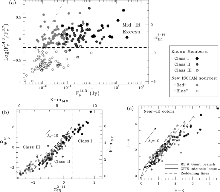
Figure 3: (a) Logarithmic ratio of the ISOCAM fluxes, log₁₀($F_{\nu}^{14.3}$/$F_{\nu}^{6.7}$), versus $F_{\nu}^{14.3}$ displayed for the 207 ISOCAM sources seen in both filters (excluding the 4 early-type young stars). The purely ISOCAM color $F_{\nu}^{14.3}$/$F_{\nu}^{6.7}$ is converted into an IR spectral index, $\alpha_{\mathrm{IR}}^{7-14}$, on the right axis, and can be used to identify sources with mid-IR excesses (above the dashed line). The completeness limit derived in Sect. 2.4 is displayed as a dotted line. (b) Mid-IR color-color diagram expressed as a spectral index diagram $\alpha_{\mathrm{IR}}^{2-7}$ versus $\alpha_{\mathrm{IR}}^{2-14}$ for 175 ISOCAM sources also detected in the K band (m_6.7 and m_14.3 on the right and upper axes are calculated as in Persi et al. pmo00 (2000)). The inclined heavy dashed line marks the limit to the right of which there is significant mid-IR excess as in (a). The two vertical dashed lines mark the formal boundary between Class II, flat-spectrum, and Class I sources (see text for details). (c) Classical near-IR color-color diagram, J–H versus H–K, for the 152 ISOCAM sources with JHK photometry.

As can be seen in Fig. 3, the mid-IR regime is ideal to detect and characterize the excess emission due to circumstellar disks around young stars. In Fig. 3a, the 207 sources detected at 6.7 $\mu$m and 14.3 $\mu$m (excluding S1, SR3, WL16, WL22) are shown in a diagram which displays the logarithmic flux ratio log₁₀($\mbox{$F_{\nu}^{14.3}$}/\mbox{$F_{\nu}^{6.7}$}$) against the mid-IR flux $F_{\nu}^{14.3}$. On the right axis of the diagram, the flux ratio $\mbox{$F_{\nu}^{14.3}$}/\mbox{$F_{\nu}^{6.7}$}$ has been converted into a classical IR spectral index, $\mbox{$\alpha_{\mathrm{IR}}$}=$ d$\log_{10}(\lambda F_{\lambda})/$d$\log_{10}(\lambda)$ (e.g. WLY89), calculated between 6.7 $\mu$m and 14.3 $\mu$m, i.e., $\alpha_{\mathrm{IR}}^{7-14}$. In this diagram, two groups of sources can clearly be distinguished. The lower ratio group has log₁₀($\mbox{$F_{\nu}^{14.3}$}/\mbox{$F_{\nu}^{6.7}$})\sim-0.7$, i.e., a spectral index on the order of $\mbox{$\alpha_{\mathrm{IR}}^{7-14}$}\sim-3.0$, which is the value expected for simple photospheric blackbody emission in the Rayleigh-Jeans regime. The dispersion around $\mbox{$\alpha_{\mathrm{IR}}^{7-14}$}\sim-3.0$ is obviously larger for weaker sources. This is mainly due to increasing photometric uncertainty with decreasing flux. The higher ratio group consists of “red” sources defined by log₁₀($\mbox{$F_{\nu}^{14.3}$}/\mbox{$F_{\nu}^{6.7}$}$) $>-0.2$ (cf. Nordh et al. nordh1 (1996)) . Most of these actually have $-0.2\leq$ log₁₀($\mbox{$F_{\nu}^{14.3}$}/\mbox{$F_{\nu}^{6.7}$})\leq 0.3$, i.e., $-1.6\lower 2.15277pt\hbox{$\;\buildrel<\over{\sim}\;$}\mbox{$\alpha_{\mathrm{IR}}^{7-14}$}\lower 2.15277pt\hbox{$\;\buildrel<\over{\sim}\;$}0$, which is typical of classical T Tauri stars (hereafter CTTS). This range of $\alpha_{\mathrm{IR}}^{7-14}$ roughly delineates the domain of Class II YSOs (e.g. Adams et al. 1987, AM94, Greene et al. 1994), and is usually interpreted in terms of optically thick circumstellar disk emission (e.g. Lada & Adams la92 (1992)). In Fig. 3, the new ISOCAM sources are distinguished from the previously known cluster members by different symbols. One can see in Fig. 3a that all the previously known Class II sources but one lie above the dividing line for red sources, while all the previously known Class III sources but two lie below it.

The object WL19, classified as a Class I YSO by WLY89 and as a reddened Class II by AM94 (see also Lada & Wilking lw84 (1984)), is here found to be a “blue” source in the mid-IR range ($\mbox{$\alpha_{\mathrm{IR}}^{7-14}$}=-1.8\pm 0.2$). This object may correspond to a luminous Class III star located behind the cloud (see also Comerón et al. crbr (1993)). Although GY12 formally has a “red” mid-IR spectral index ($\mbox{$\alpha_{\mathrm{IR}}^{7-14}$}=-0.5\pm 0.5$) here, we still consider it as a Class III object (cf. Greene et al. gwayl (1994)). (The mid-IR color is highly uncertain since GY12 is only marginaly resolved at 14.3 $\mu$m from its bright Class I neighbor GSS30.) Finally the Class III source DoAr21 has a borderline mid-IR spectral index ($\mbox{$\alpha_{\mathrm{IR}}^{7-14}$}=-1.5\pm 0.1$) but is kept as a Class III object since its color between 2.2 $\mu$m and 14.3 $\mu$m corresponds to $\mbox{$\alpha_{\mathrm{IR}}^{2-14}$}=-2.0\pm 0.1$.

A total of 71 sources are identified for the first time as mid-IR excess objects in Fig. 3a. These new “red” sources are most likely all embedded YSOs, i.e., members of the $\rho$ Ophiuchi cluster. Since dust extinction is roughly the same at 6.7 $\mu$m and 14.3 $\mu$m (Rieke & lebofsky rl (1985); Lutz lutz (1999)), any background source should be intrinsically red in order to contaminate the sample of red YSOs. Based on the Galactic model by Wainscoat et al. (wainscoat (1992)), the vast majority of background objects should appear “blue” (cf. Fig. 2). Seven background giant stars (GY45, GY65, VSSG6, GY232, GY351, GY411, and GY453 – cf. Luhman & Rieke lr99 (1999)), and a known foreground dwarf (HD148352 – Garrison garrison (1967)) are detected, which all have blue mid-IR colors ($\mbox{$\alpha_{\mathrm{IR}}^{7-14}$}=-2.7,-2.0,-3.1,-3.3,-2.9,-3.2,-3.1$, and $-3.1$, respectively).

The newly identified cloud members nicely extend the previously known Class I/II population toward low IR fluxes. While previous studies could only identify sources with $\mbox{$F_{\nu}^{14.3}$}\lower 2.15277pt\hbox{$\;\buildrel>\over{\sim}\;$}100$ mJy, the present census is complete for objects down to $\mbox{$F_{\nu}^{14.3}$}\sim 15$ mJy. Altogether, a sample of 139 Class I/Class II YSOs is identified, of which 71 are new members. The present survey has thus allowed us to more than double the number of recognized YSOs with circumstellar IR excess in the $\rho$ Ophiuchi cloud.

The 139 red YSOs are listed in Table 2 (Class I YSOs) and Table 3 (Class II YSOs) by decreasing order of $\alpha_{\mathrm{IR}}^{2-14}$. Twelve of them (last entries of Table 3) are completely new sources with respect to published IR surveys.

3.3 Class I versus Class II YSOs

In Fig. 3, the YSOs classified as Class I and Class II by AM94 and Greene et al. (gwayl (1994)) are shown as filled stars and filled circles, respectively. In the log₁₀($F_{\nu}^{14.3}$/$F_{\nu}^{6.7}$) versus $F_{\nu}^{14.3}$ diagram, there is no clear color gap between the two classes of objects, even though the Class I YSOs tend to lie in the upper part of the “red” group (see Fig. 3a). Since extinction has a negligible effect on the mid-IR ratio $F_{\nu}^{14.3}$/$F_{\nu}^{6.7}$, this suggests that Class I and Class II objects have fairly similar intrinsic colors between 6.7 $\mu$m and 14.3 $\mu$m.

The classical IR spectral index calculated from 2 $\mu$m to 10 $\mu$m (or 25 $\mu$m) (e.g. Lada & Wilking lw84 (1984) and WLY89) appears to provide a better way of discriminating between envelope-dominated Class I YSOs and disk-dominated Class II sources (see Fig. 3b). In particular, millimeter continuum mapping of optically thin circumstellar dust emission confirms that, apart from a few important exceptions (e.g., WL22, WL16, WL17, IRS37, IRS47), the $\rho$ Ophiuchi objects selected on the basis of $\mbox{$\alpha_{\mathrm{IR}}^{2-10}$}\lower 2.15277pt\hbox{$\;\buildrel>\over{\sim}\;$}0$ are indeed Class I protostars surrounded by spheroidal envelopes (AM94, MAN98).
As expected, the previously known Class I YSOs are well concentrated in the upper-right part of the $\alpha_{\mathrm{IR}}^{2-7}$ versus $\alpha_{\mathrm{IR}}^{2-14}$ diagram of Fig. 3b (where $\alpha_{\mathrm{IR}}^{2-7}$ and $\alpha_{\mathrm{IR}}^{2-14}$ are close to the $\alpha_{\mathrm{IR}}^{2-10}$ index used in previous studies – e.g., AM94 and Greene et al. gwayl (1994)). There is also a hint of two gaps in this diagram at $\mbox{$\alpha_{\mathrm{IR}}^{2-14}$}\sim 0.5$ and $\mbox{$\alpha_{\mathrm{IR}}^{2-14}$}\sim 0.0$, which roughly bracket the regime of flat-spectrum sources as defined by Greene et al. (gwayl (1994)). These may represent a distinct population of transition objects between Class I and Class II (e.g. Calvet et al. calvet94 (1994)).
Here, we thus consider sources with $\mbox{$\alpha_{\mathrm{IR}}^{2-14}$}>0.55$ as Class I YSOs (Table 2), sources with $-0.05<\mbox{$\alpha_{\mathrm{IR}}^{2-14}$}<0.55$ as candidate flat-spectrum objects (see Table 3), and sources with $\mbox{$\alpha_{\mathrm{IR}}^{2-14}$}<0.55$ as Class II YSOs (Table 3). These limiting indices are displayed in Fig. 3b. In the following, the candidate flat-spectrum sources will be treated as Class II YSOs.

3.4 Mid-IR excess versus near-IR excess

Most of the ISOCAM sources (e.g. 90 % of the Class II sources) were also detected in the near-IR (JHK) survey of Barsony et al. (bklt (1997)). Comparison between Fig. 3b and Fig. 3c illustrates the advantage of mid-IR measurements for selecting sources with intrinsic circumstellar IR excesses. While the red and blue groups of Fig. 3a are well separated in the mid-IR diagram of Fig. 3b, they blend together in the near-IR diagram of Fig. 3c.

Figure 3c also shows that most of the ISOCAM-selected YSOs lie within the reddening band associated with the intrinsic locus of CTTSs as derived by Meyer et al. (meyer97 (1997)) in Taurus. The few exceptions, which lie to the right of the reddening band, correspond to Class I and flat-spectrum YSOs.

3.5 The Class III YSO census in $\rho$ Ophiuchi

While Class I/II YSOs are easily recognized in the mid-IR range thanks to their strong IR excesses, Class III objects are difficult to identify without deep X-ray and/or radio centimeter continuum observations. We have used the ROSAT X-ray surveys of Casanova et al. (cmfa (1995)) and Grosso et al. (grosso (2000)), along with the VLA radio surveys by, e.g., André, Montmerle, & Feigelson (andre87 (1987)) and Stine et al. (stine88 (1988)) to build up a sample of bona-fide Class III YSOs covered by the present survey. With the additional Class III candidate WL19 (see Sect. 3.2 above), there are 38 such YSOs which are listed in order of decreasing $\alpha_{\mathrm{IR}}^{2-14}$ in Table 4.

This Class III sample is unfortunately not as complete as the Class I and Class II samples discussed above. According to Grosso et al. (grosso (2000)), the number of Class IIIs may be roughly as large as the number of Class IIs: above their typical X-ray detection limit of $L_{X}\sim 3\times 10^{29}$ erg s^-1 (corresponding to $L_{\star}\sim 0.3\,L_{\odot}$ – see Fig. 7 of Grosso et al.), they found a Class III/Class II number ratio of 19/22 in the $ROSAT$-$HRI$/$ISO$-$ISOCAM$ overlapping survey area. If this ratio is representative of the complete population of young stars in $\rho$ Ophiuchi, the total number of Class IIs found here (123 objects) suggests that as many as $106$ Class IIIs may be present in the cluster down to $\mbox{$L_{\star}$}\sim 0.03\,\mbox{L${}_{\odot}$}$ (our completeness level for Class IIs, see Sect. 4.4). A total of 38 Class IIIs are already known within the ISOCAM survey area, so that $\sim 68$ unknown Class IIIs may remain to be found. Since it was noted in Sect. 2.4 that $\sim 30$ sources detected at 6.7 $\mu$m might be unidentified cluster members, about half of the missing Class IIIs may have been actually seen by ISOCAM.

We also note that a large proportion (80/123) of the Class II sources are closely associated with the densest part of L1688 (see Fig. 1). Assuming the same proportion applies to Class IIIs, we would expect $\sim 44$ unknown Class III sources to be located within the CS contours of Fig. 1. A total of 39 unclassified ISOCAM sources (also detected by Barsony et al. bklt (1997)) lie within these CS contours where the number of detected background stars should be small due to high cloud extinction. Most of these 39 sources might thus be yet unidentified Class III YSOs. These candidate Class III sources are listed in order of decreasing $\alpha_{\mathrm{IR}}^{2-14}$ in Table 5.

4 Luminosity estimates and luminosity function

Most of the new YSOs identified by ISOCAM are weak IR sources which were not detected by IRAS and were not observed in previous ground-based mid-IR surveys (dedicated to bright near-IR sources). They likely correspond to low-luminosity, low-mass young stars. In Sect. 4.1 below, we derive stellar luminosity estimates for Class II and Class III objects using published near-IR photometry from Barsony et al. (1997). In Sect. 4.2, we provide mid-IR estimates of the disk luminosities, $L_{\mathrm{disk}}$, for Class II YSOs. Finally, calorimetric estimates of the bolometric luminosities, $L_{\mathrm{bol}}$, for Class I YSOs are calculated in Sect. 4.3. The luminosity function of the $\rho$ Ophiuchi embedded cluster is then assembled in Sect. 4.4.

4.1 Dereddened J-band stellar luminosities for Class II and Class III sources

The J-band flux provides a good tracer of the stellar luminosity for late-type PMS stars (i.e., T Tauri stars) because the J-band is close to the maximum of the photospheric energy distribution for such cool stars. It is also a good compromise between bands too much affected by interstellar extinction at short wavelengths (very few $\rho$ Ophiuchi YSOs have been detected in the V, R, or I bands), and the H, K and mid-IR bands which are contaminated by intrinsic excesses. Greene et al. (gwayl (1994)) showed that there is a good correlation between the dereddened J-band flux and the stellar luminosity derived by other methods. They pointed out that in $\rho$ Ophiuchi this correlation is roughly consistent with a more theoretically based correlation expected for 1-Myr old PMS stars following the D’Antona & Mazzitelli (dm94 (1994)) evolutionary tracks. More recently, Strom et al. (sks (1995)) and Kenyon & Hartmann (kh95 (1995)) used the same model PMS tracks to directly convert dereddened J-band fluxes into stellar masses. We adopt a similar approach here.

4.1.1 Extinction estimates from near-IR colors

The main difficulty and source of uncertainty with this method is due to the foreground extinction affecting the J-band fluxes. One must estimate the interstellar extinction toward each source in order to correct the observed J-band fluxes. We have used the observed near-IR colors to estimate the J-band extinction. The $(J-H)$ color excess is most suitable for this purpose (e.g. Greene et al. gwayl (1994)) since the dispersion in the intrinsic $(J-H)$ colors of CTTSs is small and observationally well determined (cf. Strom et al. strom89 (1989), Meyer et al. meyer97 (1997)).

The reddening law quoted by Cohen et al. (cohen (1981)), which is determined for the standard CIT system, should be applicable to the JHK photometry of Barsony et al. (bklt (1997)). We have thus used:

$$A_{V}=9.09\times[(J-H)-(J-H)_{0}]$$$$ (1)

when the $(J-H)$ color is available, and

$$A_{V}=15.4\times[(H-K)-(H-K)_{0}]$$ (2)

otherwise, where we have adopted $(J-H)_{0}=0.85$, and $(H-K)_{0}=0.55$ from the CTTS results of Meyer et al. (meyer97 (1997)). The dereddened $J_{0}$ magnitude is then obtained as $J_{0}=J-0.265\times A_{V}$, or $H_{0}=H-0.155\times A_{V}$ for those stars not detected in J (with $A_{V}$ estimated from H–K). The dereddened $J_{0}$ (or $H_{0}$) can then be converted into an absolute J-band (H-band) magnitude, $M_{J}$ ($M_{H}$), via the distance modulus of the $\rho$ Ophiuchi cloud equal to 5.73 (for $d=140$ pc).

The uncertainties on $M_{J}$ and $M_{H}$ result from the typical uncertainties on the J, H, K magnitudes and on the intrinsic colors $(J-H)_{0}$ and $(H-K)_{0}$. With $\sigma(J)=0.1$, $\sigma(H)\sim\sigma(K)=0.05$ (Barsony et al. bklt (1997)), and $\sigma$($(J-H)_{0}$)$\,=0.1$, $\sigma$($(H-K)_{0}$)$\,=0.2$ (Meyer et al. meyer97 (1997)), we obtain the following typical uncertainties: $\sigma$($M_{J}$) $=0.39$ mag, and $\sigma$($M_{H}$) $=0.60$ mag. In addition, the uncertainty on the cluster distance ($140\pm 10$ pc) induces a maximum systematic error of $\pm 0.15$ mag on $M_{J}$ and $M_{H}$.

4.1.2 Relationship between $M_{J}$ and $L_{\star}$ for young T Tauri stars

The absolute J-band magnitude $M_{J}$ can be directly converted into a stellar luminosity $L_{\star}$ if the effective stellar temperature $T_{\mathrm{eff}}$ is known: $\log_{10}(\mbox{$L_{\star}$})=1.89-0.4\times(M_{J}+BC_{J}(\mbox{$T_{\mathrm{eff}}$}))$, where BC_J is the bolometric correction for the J band depending only on $T_{\mathrm{eff}}$. Pre-main sequence objects in the mass range $0.1\lower 2.15277pt\hbox{$\;\buildrel<\over{\sim}\;$}M_{\star}\lower 2.15277pt\hbox{$\;\buildrel<\over{\sim}\;$}2.5\,M_{\odot}$ are cool sub-giant stars with typical photospheric temperatures $\mbox{$T_{\mathrm{eff}}$}\sim$ 2500–5500 K (e.g. Greene & Meyer gm95 (1995), D’Antona & Mazzitelli dm94 (1994)). In this temperature range (0.34 dex wide), the photospheric blackbody peaks close to the J band (1.2$\mu$m), so that the J–band bolometric correction spans only a limited range, $1\lower 2.15277pt\hbox{$\;\buildrel<\over{\sim}\;$}BC_{J}\lower 2.15277pt\hbox{$\;\buildrel<\over{\sim}\;$}2$, corresponding to a total shift in luminosity of only 0.4 dex. Therefore, if we use a (geometrical) average value for the effective temperature, $\mbox{$T_{\mathrm{eff}}$}^{0}\sim 3700$ K, we should not make an error larger than $\pm 0.2$ dex on $\log_{10}(\mbox{$L_{\star}$})$.

Figure 4: $M_{J}-$ log₁₀($T_{\mathrm{eff}}$) “HR” diagram showing the well-defined strip of the HR diagram occupied by the PMS tracks of D’Antona & Mazzitelli (1998). For $M_{J}=4.0$ for instance, we see that log₁₀($T_{\mathrm{eff}}$) can span a range of only $\sim 0.15$ dex for stellar ages between $0.1\,$Myr and $3\,$Myr. We thus adopt the $M_{J}-$ log₁₀($T_{\mathrm{eff}}$) linear relationship displayed as a heavy dashed line which corresponds to the conversion: $\log_{10}(\mbox{$L_{\star}$})=1.49-0.466\times M_{J}$.

Furthermore, since bright $M_{J}$ sources tend to be of earlier spectral type than faint sources, we can in fact achieve more accurate luminosity estimates. Indeed, PMS stars are predicted to lie within a well-defined strip of the HR diagram. This is illustrated in Fig. 4 which displays model evolutionary tracks and isochrones from D’Antona & Mazzitelli (dm97 (1998)) on a $M_{J}$–log${}_{10}(\mbox{$T_{\mathrm{eff}}$})$ diagram for PMS stars with ages between $0.1\,$Myr and $3\,$Myr. We have used the compilations of Hartigan et al. (hss94 (1994)), Kenyon & Hartmann (kh95 (1995)), and Wilking et al. (wgm (1999)) to derive an approximate linear interpolation for $BC_{J}$: $BC_{J}=1.65+3.0\times$log₁₀($3700/\mbox{$T_{\mathrm{eff}}$}$). Figure 4 shows that, for a given observed value of $M_{J}$, the possible range of log₁₀($T_{\mathrm{eff}}$) is reduced to less than $\sim$ 0.15 dex, inducing a maximum error of $\pm 23\,$% ($\pm 0.09$ dex) on $L_{\star}$. Based on Fig. 4, we have adopted a linear relationship between $M_{J}$ and $T_{\mathrm{eff}}$: log$(\mbox{$T_{\mathrm{eff}}$}/3700)=-0.055\times(M_{J}-4.0)$ (see the heavy dashed line in Fig. 4). This leads to the following $\mbox{$L_{\star}$}-M_{J}$ conversion:

$$\log_{10}(\mbox{$L_{\star}$})=1.49-0.466\times M_{J}.\hskip 19.91684pt$$ (3)

The uncertainty resulting from this conversion should be on the order of 0.045 dex for $0.01\leq\mbox{$L_{\star}$}\leq 10.0\,\mbox{L${}_{\odot}$}$. We therefore estimate that the total uncertainty on $\log_{10}(\mbox{$L_{\star}$})$ is $\sigma$($\log_{10}\mbox{$L_{\star}$}$) $=(0.045^{2}+(0.466\times\sigma$($M_{J}$)$)^{2})^{1/2}$ $=0.19$ dex.

The $\mbox{$L_{\star}$}-M_{J}$ conversion described above cannot be applied to sources undetected in the J band. Instead, we use the H-band magnitude, along with the extinction estimate derived from the $(H-K)$ color, but with the additional complication that the circumstellar (disk) emission cannot be neglected. Meyer et al. (meyer97 (1997)) found that the H-band circumstellar excess is on the order of 20 % of the stellar flux, on average, for the Taurus CTTS sample of Strom et al. (strom89 (1989)) (for a $\rho$ Ophiuchi sample, see Greene & Lada gl96 (1996)). This excess, expressed as a veiling index $r_{H}=F_{\nu}\!\!^{H}{}_{\hskip 2.84544pt\mathrm{exc}}/F_{\nu}\!\!^{H}{}_{\hskip 2.84544pt\star}$ (e.g. Greene & Meyer gm95 (1995)), is equal to $\sim 0.2$. Accordingly, we have applied a systematic correction $\delta$H $=\,-2.5\,\log_{10}(1+r_{H})\sim 0.2$ mag. The $\mbox{$L_{\star}$}-M_{H}$ relationship obtained in a way similar to the J-band relation is then:

$$\log_{10}(\mbox{$L_{\star}$})=1.26-0.477\times(M_{H}+0.2)$$ (4)

The total uncertainty on $\log_{10}(\mbox{$L_{\star}$})$ derived from $M_{H}$ is then $\sigma$($\log_{10}\mbox{$L_{\star}$}$) $=(0.045^{2}+(0.477\times\sigma$($M_{H}$)$)^{2})^{1/2}$ $=0.29$ dex.

This method can also be applied to Class III YSOs, using different values for $(J-H)_{0}$ and $(H-K)_{0}$. We have derived $L_{\star}$ for all Class III YSOs using the following relationships: $A_{V}=9.09\times[(J-H)-0.6]$, or $A_{V}=15.4\times[(H-K)-0.15]$; and log$(\mbox{$L_{\star}$})=1.49-0.466\times(J-0.265\times A_{V}-5.73)$, or log$(\mbox{$L_{\star}$})=1.26-0.477\times(H-0.155\times A_{V}-5.73)$ (the H-band IR excess for Class III YSOs is negligible).
The resulting $M_{J},M_{H},A_{V}$, and $L_{\star}$ estimates are listed in Table 3 for Class II YSOs, and in Table 4 and Table 5 for Class III YSOs.

4.2 Disk luminosities for Class II YSOs

Since the SED of an embedded Class II YSO peaks in the mid-IR range, the ISOCAM fluxes should be approximately valid tracers of the total, bolometric luminosities ($L_{\mathrm{bol}}$). To estimate $L_{\mathrm{bol}}$ for weak Class II sources, an empirical approach thus consists in using this $F_{\nu}^{\mathrm{MIR}}$–$L_{\mathrm{bol}}$ relationship after proper calibration on a sub-sample of (brighter) objects for which the luminosity can be derived by a more direct method. This approach has been adopted by, e.g., Olofsson et al. (ohk99 (1999)). Here, we have used the $L_{\star}$ estimates of Sect. 4.1 to check that a correlation is actually present between $L_{\star}$ and the mid-IR fluxes. Figure 5 displays $F_{\nu}^{14.3}$ (corrected for extinction) as a function of $L_{\star}$ for the 104 Class II sources detected both in the near-IR and in the mid-IR range.

Figure 5: Correlation between $F_{\nu}^{14.3}$ (corrected for interstellar extinction with $A_{14.3}=0.03\times\mbox{$A_{V}$}$) and $L_{\star}$. The observations are compared with a purely reprocessing disk model with $\mbox{$L_{\mathrm{disk}}$}=0.25\times\mbox{$L_{\star}$}$ and a stellar contribution given by Eq. 6. The continuous line corresponds to an average disk inclination ($i=60\degr$), while the dotted and dashed lines correspond to more extreme inclinations ($i=0\degr$ and $i=85\degr$).

A correlation is found, showing that, despite some scatter, the ISOCAM fluxes can be used to give rough estimates of the stellar luminosities of Class II YSOs. This is useful for the few ISOCAM sources of our sample which have not been detected at near-IR wavelengths.

The mid-IR emission of Class II YSOs is usually interpreted as arising from warm dust in an optically thick circumstellar disk. Using a simplified disk model (e.g. Beckwith et al. beckwith90 (1990)), it is easy to show that any observed monochromatic flux in the optically thick, power-law range of the disk SED is simply proportional to the total disk luminosity $L_{\mathrm{disk}}$ divided by the projection factor cos($i$), where $i$ is the disk inclination angle to the line of sight. In the Beckwith et al. (1990) model, the disk is parameterized by a power-law temperature profile with three free parameters, $T_{0}$, $r_{0}$, and $q$, such that: $T(r)=T_{0}\times(r/r_{0})^{-q}$. Here, we have adopted $T_{0}=1500$ K, meaning that the disk inner radius is at the dust sublimation temperature, and $q=2/3$, corresponding to an IR spectral index $\mbox{$\alpha_{\mathrm{IR}}$}=2/q-4=-1.0$ typical of CTTS spectra.

We must, however, account for the fact that the stellar emission itself is not completely negligible in the mid-IR bands, especially at 6.7 $\mu$m. A simple blackbody emission at $T_{\star}=3700$ K gives

$$F_{\nu\hskip 2.84544pt\star}^{\,\,\,6.7}=0.082\times(\mbox{$L_{\star}$}/1\,\mbox{L${}_{\odot}$})\,\,\mathrm{Jy}$$ (5)

$$\mbox{$F_{\nu\hskip 2.84544pt\star}^{14.3}$}=0.021\times(\mbox{$L_{\star}$}/1\,\mbox{L${}_{\odot}$})\,\,\mathrm{Jy}.$$ (6)

Since $F_{\nu\hskip 2.84544pt\star}^{14.3}$ is significantly smaller than $F_{\nu\hskip 2.84544pt\star}^{6.7}$, only $F_{\nu}^{14.3}$ is used to estimate $L_{\mathrm{disk}}$. Assuming cos$(i)=0.5$ ($i=60\degr$) in all cases, we have computed $L_{\mathrm{disk}}$ for each of the Class II YSOs with $L_{\star}$ and $A_{V}$ estimates from Sect. 4.1, based on the following relationship:

$$\mbox{$L_{\mathrm{disk}}$}/1\,\mbox{L${}_{\odot}$}=(\mbox{$F_{\nu}^{14.3}$}\times 10^{+0.4\times A_{14.3}}-\mbox{$F_{\nu\hskip 2.84544pt\star}^{14.3}$})/1.80\,\mathrm{Jy},$$ (7)

where $A_{14.3}\!=\!0.03\times\mbox{$A_{V}$}$ and $F_{\nu\hskip 2.84544pt\star}^{14.3}$ from Eq. 6. The results are given in the last column of Table 3.

According to this model, the mid-IR flux is a direct tracer of the disk luminosity, and the $F_{\nu}^{\mathrm{MIR}}-\mbox{$L_{\star}$}$ correlation of Fig. 5 simply expresses that $L_{\mathrm{disk}}$ correlates with $L_{\star}$. The origin of $L_{\mathrm{disk}}$ is either the release of gravitational energy by accretion in the disk, or the absorption/reprocessing of stellar photons by the dusty disk. In the latter case, $L_{\mathrm{disk}}$ is naturally proportional to $L_{\star}$. The fraction $\mbox{$L_{\mathrm{disk}}$}/\mbox{$L_{\star}$}$ of stellar luminosity reprocessed by the disk depends on the spatial distribution of dust. In the ideal case of an infinite, spatially flat disk, this fraction is 0.25 (Adams & Shu as86 (1986)). If the disk is flared, $\mbox{$L_{\mathrm{disk}}$}/\mbox{$L_{\star}$}$ is larger, while it is smaller if the disk has a inner hole. The theoretical $F_{\nu}^{\mathrm{MIR}}-\mbox{$L_{\star}$}$ correlations plotted in Fig. 5 correspond to $\mbox{$L_{\mathrm{disk}}$}=0.25\times\mbox{$L_{\star}$}$ and to three representative inclination angles. The fact that this simple model accounts for the observed correlation quite well, suggests that the disks of most $\rho$ Ophiuchi Class II YSOs are passive disks dominated by reprocessing. This is consistent with recent estimates of the disk accretion level in Taurus CTTSs (e.g. Gullbring et al. gullbring (1998)). The typical disk accretion rate of a CTTS is estimated to be $10^{-8}\,\mbox{M${}_{\odot}$}/$yr, corresponding to an accretion luminosity $\mbox{$L_{\mathrm{acc}}$}=0.025\,\mbox{L${}_{\odot}$}$ for $\mbox{$R_{\star}$}=3\,\mbox{R${}_{\odot}$}$ and $\mbox{$M_{\star}$}=0.25\,\mbox{M${}_{\odot}$}$ (i.e., $\mbox{$L_{\star}$}\sim 0.25\,\mbox{L${}_{\odot}$}$ at 1 Myr). In this case, the luminosity due to reprocessing is $\sim 5$ times larger than the accretion luminosity in the disk.

On the other hand, 37 sources (among a total of 104) are located above the passive disk model lines in Fig. 5. These are good candidates for having an active disk with an accretion rate typically larger than $\sim 5\times(\mbox{$L_{\star}$}/0.25\mbox{L${}_{\odot}$})\times 10^{-8}\,\mbox{M${}_{\odot}$}/$yr.

Overall, we find that the median $\mbox{$L_{\mathrm{disk}}$}/\mbox{$L_{\star}$}$ ratio is 0.41 for the 93 Class II sources detected in the near-IR and with $\mbox{$F_{\nu}^{14.3}$}>\,15\,$mJy (i.e. the completeness level derived in Sect. 2.4). Using this ratio, we have derived rough estimates of the stellar luminosities of the 15 Class II YSOs which have no near-IR photometry (see Table 3) as follows:

$$\mbox{$L_{\star}$}(\mbox{L${}_{\odot}$})\approx\mbox{$L_{\mathrm{disk}}$}/0.41\approx(0.97\times 1.6/0.41)\times(\mbox{$F_{\nu}^{14.3}$}/1.8\,\mathrm{Jy}).$$ (8)

[The factor 0.97 corresponds to a typical stellar contribution of $3\,$% at 14.3 $\mu$m, while the factor 1.6 is an average extinction correction at 14.3 $\mu$m (corresponding to $<A_{V}>=17$ mag).]

4.3 Calorimetric luminosities for Class I sources

The most direct method of estimating the total luminosities $L_{\mathrm{bol}}$ of embedded YSOs consists in integrating the observed SEDs (cf. WLY89). However, since most of the $\rho$ Ophiuchi Class II and Class III YSOs are deeply embedded within the cloud ($A_{V}\lower 2.15277pt\hbox{$\;\buildrel>\over{\sim}\;$}10$), only a negligible fraction of their bolometric luminosity can be recovered by finite-beam IR observations (e.g. Comerón et al. crbr (1993)). We thus do not attempt to derive calorimetric estimates of $L_{\mathrm{bol}}$ for these sources. In contrast, the calorimetric method is believed to be appropriate for Class I YSOs since these are self-embedded in substantial amounts of circumstellar material which re-radiate locally the absorbed luminosity (cf. WLY89 and AM94). Using our new mid-IR measurements, we have evaluated the calorimetric luminosities ($L_{\mathrm{cal}}$) of the 16 Class I YSOs observed in our survey. Only 7 of them have reliable IRAS fluxes up to 60 or 100 $\mu$m (IRS54, IRS44, GSS30, IRS43, EL29, IRS48, IRS51). For these, the median of the ratio of $L_{\mathrm{cal}}$(6.7–14.3$\mu$m) to $L_{\mathrm{bol}}$ is found to be 9.8, suggesting that the typical fraction of a Class I source’s luminosity radiated between 6.7 and 14.3 $\mu$m is $\sim 10$ % . Assuming that this ratio is representative of all Class I YSOs, we have derived estimates of $L_{\mathrm{bol}}$ for the remaining 9 weaker Class I sources (i.e., CRBR85, LFAM26, LFAM1, WL12, IRS46, CRBR12, IRS67, CRBR42, WL6). These luminosities are listed in Table 2.

4.4 Luminosity function of the $\rho$ Ophiuchi embedded cluster

Combining the $L_{\star}$ luminosities determined in Sect.  4.1 for the sources detected in the near-IR with the $L_{\star}$ estimates from $L_{\mathrm{disk}}$ for the sources without near-IR measurements (Sect. 4.2), we have built a luminosity function for Class II YSOs which represents a major improvement over previous studies (see Fig. 6a). In terms of $L_{\star}$, the completeness level for this population can be estimated from the $F_{\nu}^{14.3}$ completeness limit derived in Sect. 2.4 ($\mbox{$F_{\nu}^{14.3}$}\sim 15\,$mJy) using Eq. 8: $\mbox{$L_{\star}$}^{comp}(\rm{ClassII})=0.032\,\mbox{L${}_{\odot}$}$. While the luminosity function previously published by Greene et al. (gwayl (1994)) included only 33 (bright) Class II sources and suffered from severe incompleteness below $\mbox{$L_{\star}$}\sim 1-2\,\mbox{L${}_{\odot}$}$, our present completeness level is a factor $\sim$ 30–50 lower. The new luminosity function shows a marked flattening in logarithmic units at $\mbox{$L_{\star}$}\sim 2\,\mbox{L${}_{\odot}$}$, well above our completeness limit. This important new feature is discussed in Sect. 5 below.

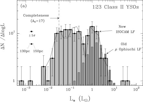
Figure 6: Luminosity functions (LF) (a) for the 123 Class II YSOs (continuous histogram with statistical error bars). The function corresponding to a similar histogram shifted by half the 0.2 dex bin size is shown as a thin curve to illustrate the level of statistical fluctuations due to binning. The LF of 33 Class II sources from Greene et al. (1994) is displayed as a darker histogram (rebinned to 0.2 dex bins, and rescaled to $d=140$ pc for better comparison with the new LF). The typical $\pm 1\sigma$ uncertainty on the position of each bin resulting from the individual uncertainties on $L_{\star}$ is indicated, along with the effect of the distance uncertainty; (b) for the 16 Class I YSOs ; and (c) for the sample of 55 (19 confirmed $+$ 36 candidate) Class III sources from Table 4 and 5. The LF of (a) is shown in the background for comparison. The dashed vertical lines show the respective completeness levels.

Based on the $L_{\mathrm{cal}}$ estimates of Sect. 4.3, a new bolometric luminosity function for the 16 Class I YSOs of $\rho$ Ophiuchi is displayed in Fig. 6b. The associated completeness level is derived from $\mbox{$F_{\nu}^{6.7}$}=10\,$mJy and $\mbox{$F_{\nu}^{14.3}$}=15\,$mJy (Sect. 2.4) using $\mbox{$L_{\mathrm{bol}}$}/\mbox{$L_{\mathrm{cal}}$}$(6.7–14.3$\mu$m)$\approx 9.8$ (Sect. 4.3): $\mbox{$L_{\star}$}^{\mathrm{comp}}(\rm{ClassI})=0.017\,\mbox{L${}_{\odot}$}$. The median $L_{\mathrm{bol}}$ for Class I YSOs is $1.6\ \mbox{L${}_{\odot}$}$, which is $\sim 8$ times larger than the median $L_{\star}$ of Class II YSOs ($0.20\,\mbox{L${}_{\odot}$}$). The luminosities of Class I YSOs span a range of two orders of magnitude between $\sim 0.1\ \mbox{L${}_{\odot}$}$ and $\sim 10\ \mbox{L${}_{\odot}$}$, which is roughly as wide as the luminosity range spanned by Class II YSOs. The comparatively large value of $L_{\mathrm{bol}}$ for Class I YSOs is probably due to a dominant contribution of accretion luminosity as expected in the case of protostars.

In Fig. 6c, we plot the luminosity function of the 55 Class III sources that are located within the CS contours of Fig. 1 and for which we have enough near-IR data to derive $L_{\star}$ according to the procedure described in Sect. 4.1. This sample comprises 19 confirmed Class IIIs from Table 4 together with 36 candidate Class III sources from Table 5. It might be contaminated by a few background/foreground sources but is characterized by a relatively well defined completeness luminosity. From the completeness level $\mbox{$F_{\nu}^{6.7}$}=10\,$mJy and using Eq. 5 with an average extinction correction corresponding to $A_{V}=17$ mag, we get $\mbox{$L_{\star}$}^{comp}(\rm{ClassIII})=0.20\,\mbox{L${}_{\odot}$}$, which is $\sim 6$ times higher than $\mbox{$L_{\star}$}^{comp}(\rm{ClassII})$. Deep X-ray observations with $XMM$ should improve the completeness luminosity for Class III YSOs by an order of magnitude in the near future (cf. discussion by Grosso et al. grosso (2000) in a companion paper).

5 Modeling of the luminosity function

If the mass-luminosity relationship of PMS stars were a simple, fixed power-law function, the shape of the luminosity function would directly reflect the underlying mass function. Unfortunately, the mass-luminosity relation is a complex function with inflexion points and is strongly age-dependent. Deriving the mass function from the luminosity function thus requires knowledge of the stellar age distribution. The $\rho$ Ophiuchi embedded cluster is believed to be younger than most known star clusters (e.g. Luhman & Rieke lr99 (1999)), with a typical age on the order of, or less than, 1 Myr (e.g. WLY89, Greene & Meyer gm95 (1995)).

The 123 Class II sources identified with ISOCAM are presently the most complete sample of young stars available in the cluster. The corresponding mass function is estimated down to $0.055\,\mbox{M${}_{\odot}$}$ in Sect. 5.1. We investigate the effect of including Class III YSOs by modeling the luminosity function of the 135 Class II and Class III objects located inside the CS contours of Fig. 1 (Sect. 5.3).

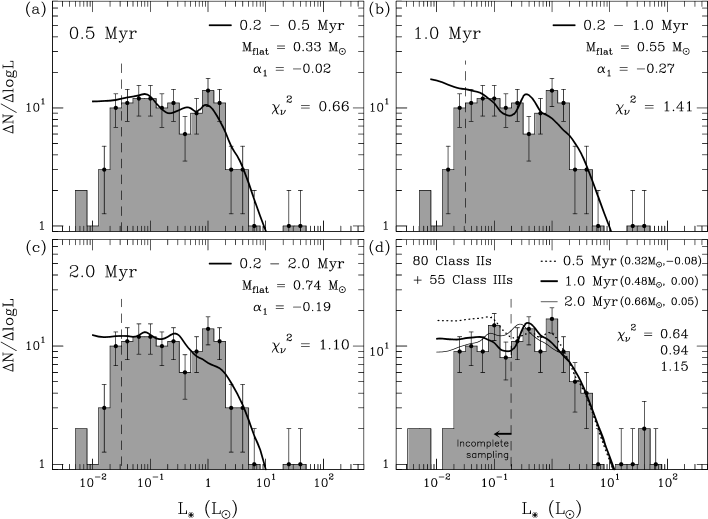
Figure 7: Best model fits (heavy curves) to the luminosity function of Class II sources obtained for a stellar age distribution corresponding to a constant formation rate over (a) 0.5 Myr, (b) 1 Myr, and (c) 2 Myr (the first 0.2 Myr have been avoided in the PMS tracks to account for a typical protostellar timescale). In (d), similar best fits are shown for the combined luminosity function of 135 Class II and Class III sources inside the CS contours of Fig. 1. The vertical dashed lines show the completeness levels of the respective luminosity functions (see Fig. 6).

5.1 Constraints on the mass function of Class II YSOs

We have modeled the observed luminosity function using a two-segment power-law mass function with two free parameters, $M_{\mathrm{flat}}$ and $\alpha_{1}$: d$N/$d log$\mbox{$M_{\star}$}\propto\mbox{$M_{\star}$}^{\alpha_{1}}$ for $\mbox{$M_{\star}$}<\mbox{$M_{\mathrm{flat}}$}$, and d$N/$d log$\mbox{$M_{\star}$}\propto\mbox{$M_{\star}$}^{-1.7}$ for $\mbox{$M_{\star}$}>\mbox{$M_{\mathrm{flat}}$}$. The high-mass range (for $\mbox{$M_{\star}$}>\mbox{$M_{\mathrm{flat}}$}$) is simply taken to be a power-law with index $-1.7$ (whereas the Salpeter index would be $-1.35$), in agreement with the IMFs favored by Kroupa et al. (kroupa (1993)) and Scalo (scalo (1998)). We assume that the cluster forms stars with a fixed IMF, independent of time. The evolutionary tracks of D’Antona & Mazzitelli (dm97 (1998)) are used to derive a set of mass-luminosity relations adapted to the $\rho$ Ophiuchi PMS population, under the following three hypotheses about the star formation history: Constant star formation rate over a) 0.5 Myr (Fig. 7a), b) 1 Myr (Fig. 7b), and c) 2 Myr (Fig. 7c). Cases b) and c) correspond to the simplest scenarios consistent with current observational constraints (e.g. WLY89). Case a) mimics a recent “burst” of star formation suggested by recent studies (e.g. Greene & Meyer gm95 (1995) and Luhman & Rieke lr99 (1999)). These three scenarios are roughly representative of our current (imperfect) knowledge of the stellar age distribution in the cluster.

The fitting analysis is performed on the 12 (logarithmic) luminosity bins above the completeness level of 0.032 L_⊙ and below $10\,\mbox{L${}_{\odot}$}$ by varying $\alpha_{1}$ and $M_{\mathrm{flat}}$. Due to the age ambiguity for a particular ($M_{\star}$, $L_{\star}$) in the PMS tracks for $\mbox{$M_{\star}$}\lower 2.15277pt\hbox{$\;\buildrel>\over{\sim}\;$}2\,\mbox{M${}_{\odot}$}$ and $age<3\,$Myr as a result of the transition from convective to radiative interiors (e.g. Fig. 4), our simplified modeling is not valid for $\mbox{$L_{\star}$}\lower 2.15277pt\hbox{$\;\buildrel>\over{\sim}\;$}10\,\mbox{L${}_{\odot}$}$. The best fit is shown as a heavy curve for each of the three assumed age distributions (Fig. 7a, 7b, and 7c). The flattening of the luminosity function below $2\ \mbox{L${}_{\odot}$}$ is well reproduced in all three cases. The best-fit model in the 1 Myr case (Fig. 7b) is however not quite as good as the two others since it predicts a peak at $\mbox{$L_{\star}$}\sim 0.4-0.5\,\mbox{L${}_{\odot}$}$ where the data show a dip. This is reflected by the largest value $1.41$ for the reduced $\mbox{$\chi^{2}\!\!_{\nu}$}\equiv\frac{\chi^{2}}{N-n}$ (with $N=12$ fitted data points and $n=2$ free parameters). The model of Fig. 7c reproduces the data somewhat better ($\mbox{$\chi^{2}\!\!_{\nu}$}=1.10$) as the predicted peak luminosity moves down to $\mbox{$L_{\star}$}\sim 0.2-0.3\,\mbox{L${}_{\odot}$}$. A marginally better fit is obtained with the 0.5 Myr model (Fig. 7a, $\mbox{$\chi^{2}\!\!_{\nu}$}=0.66$). In this case, the model luminosity function has a local maximum at $\mbox{$L_{\star}$}\lower 2.15277pt\hbox{$\;\buildrel>\over{\sim}\;$}1\,\mbox{L${}_{\odot}$}$ as observed and the flattening for $\mbox{$L_{\star}$}\sim 2\,\mbox{L${}_{\odot}$}$ is particulary well reproduced.

The best-fit values of $M_{\mathrm{flat}}$ along with the formal $1\,\sigma$ errors resulting from the fitting procedure are as follows: $0.33\pm 0.04\,\mbox{M${}_{\odot}$}$, $0.55\pm 0.09\,\mbox{M${}_{\odot}$}$, and $0.74\pm 0.13\,\mbox{M${}_{\odot}$}$ for Fig. 7a, 7b, and 7c, respectively. These $M_{\mathrm{flat}}$ values follow the expected trend that the older the stars, the higher the derived masses for the same luminosities. The final error on the determination of $M_{\mathrm{flat}}$ is clearly dominated by the uncertainties on the stellar age distribution. We adopt the following average value: $\mbox{$M_{\mathrm{flat}}$}=0.55\pm 0.25\,\mbox{M${}_{\odot}$}$. The best-fit values for $\alpha_{1}$ are $-0.02\pm 0.15$, $-0.27\pm 0.13$, and $-0.19\pm 0.13$, respectively. There is no correlation with age in this case. We conservatively adopt $\alpha_{1}=-0.15\pm 0.2$. These constraints on the mass function are valid for $0.032\,\mbox{L${}_{\odot}$}<\mbox{$L_{\star}$}<10\,\mbox{L${}_{\odot}$}$, which approximately corresponds to $0.055\,\mbox{M${}_{\odot}$}\lower 2.15277pt\hbox{$\;\buildrel<\over{\sim}\;$}\mbox{$M_{\star}$}\lower 2.15277pt\hbox{$\;\buildrel<\over{\sim}\;$}2\,\mbox{M${}_{\odot}$}$.

Under the same three assumptions about the stellar age distribution as above, we have also derived a range of stellar masses directly from the $M_{J}$ magnitude for each of the 123 Class II YSOs. We display the results as a mass function in Fig. 8, where the vertical error bars reflect the uncertainties induced by the various age assumptions rather than the statistical errors. The best two-component power-law mass function derived above is superposed as a heavy curve. The error bars are particulary large for the two mass bins close to 1 M_⊙, i.e., just above $M_{\mathrm{flat}}$. This is due to a shift of a large number of stars beyond $M_{\mathrm{flat}}$ when the stellar ages are varied upward. The global shape of the mass function is however fairly well determined: It is basically flat (in logarithmic units) at low masses down to 0.055 M_⊙ and shows a steep decline beyond $\sim 0.5\,\mbox{M${}_{\odot}$}$.

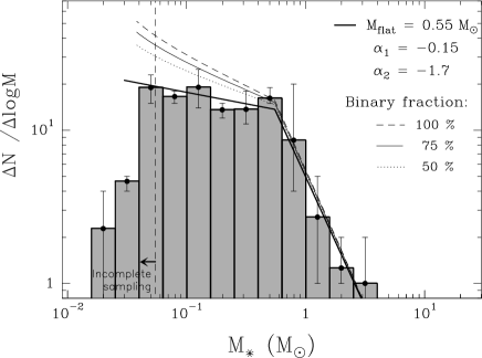
Figure 8: Mass function of the 123 Class II YSOs. The range of possible age distributions (see Sect. 5.1) induces a range of masses for each star and thus an uncertainty on the derived histogram displayed as vertical error bars. The best two-segment power-law mass function of Sect. 5.1 (heavy solid curve), and the effect of binarity as a function of the binary fraction from 50 % to 100 % (light curves – see Sect. 6.2) are shown. The vertical dashed line marks the completeness level of $0.055\,\mbox{M${}_{\odot}$}$.

5.2 Possible deuterium feature in the luminosity function of Class II YSOs

Some of the features (peaks and dips) apparent in the observed luminosity function might be real as they are also predicted by the models (see Fig. 7). The feature expected in the luminosity function of young stars as a result of deuterium burning during PMS contraction is particularly interesting since its location is age-dependent (e.g. Zinnecker et al. zinnecker (1993)). As already noted, the model fit obtained under the 0.5 Myr scenario is particularly good as it predicts a peak at $\mbox{$L_{\star}$}\sim 1.5\,\mbox{L${}_{\odot}$}$, consistent with the observations (see Fig. 7a). In the model, this $1.5\,\mbox{L${}_{\odot}$}$ peak corresponds to an inflexion point in the mass-luminosity relation due to deuterium burning in $\sim 0.4$-Myr old stars with $\mbox{$M_{\star}$}\sim 0.5\,\mbox{M${}_{\odot}$}$. If this peak in the luminosity function is confirmed, it will provide strong evidence that the population of Class II YSOs is particularly young in $\rho$ Ophiuchi.

5.3 Effect of Class III YSOs

There is most probably a significant population of Class III objects embedded in the cloud (e.g. Sect. 3.5). To evaluate how the presence of this population may affect our conclusions on the IMF of the cluster (see Sect. 6 below), we here consider the luminosity function of a combined sample of Class II and Class III sources. The sample comprises the 80 Class II and 55 Class III YSOs located inside the CS contours of Fig. 1. It should be complete down to $\sim 0.2\,\mbox{L${}_{\odot}$}$. (Note, however, that only 19 of the 55 Class III sources of this sample are confirmed YSOs at this stage – see Sect. 4.4.) The associated luminosity function, displayed in Fig. 7d, is very similar to the luminosity function of Class II YSOs. In particular, it exhibits a flattening below $\sim 1-2\,\mbox{L${}_{\odot}$}$.

The results of a modeling similar to that of Sect. 5.1, but performed on only 8 luminosity bins between 0.2 and 10 L_⊙, are shown in Fig. 7d. The best fits found under the same three star formation scenarios as in Sect. 5.1 are good (with $\mbox{$\chi^{2}\!\!_{\nu}$}=0.64$, 0.94, and 1.15, respectively). The best-fit values for the parameters $M_{\mathrm{flat}}$ and $\alpha_{1}$ of the mass function are as follows: $\mbox{$M_{\mathrm{flat}}$}=0.32\pm 0.04\,\mbox{M${}_{\odot}$}$, $0.48\pm 0.08\,\mbox{M${}_{\odot}$}$, $0.66\pm 0.10\,\mbox{M${}_{\odot}$}$, and $\alpha_{1}=-0.08\pm 0.45$, $0.00\pm 0.35$, $+0.05\pm 0.19$ for star formation durations of 0.5, 1, and 2 Myr, respectively. Combining these results, we obtain $\mbox{$M_{\mathrm{flat}}$}\sim 0.5\pm 0.2\,\mbox{M${}_{\odot}$}$ and $\alpha_{1}\sim 0.0\pm 0.4$. Within the uncertainties these values are essentially identical to those found in Sect. 5.1 for the sample of Class II YSOs, although they apply to a more limited mass range, approximately $0.17\,\mbox{M${}_{\odot}$}\lower 2.15277pt\hbox{$\;\buildrel<\over{\sim}\;$}\mbox{$M_{\star}$}\lower 2.15277pt\hbox{$\;\buildrel<\over{\sim}\;$}2\,\mbox{M${}_{\odot}$}$.

In contrast to the Class II case, the luminosity function of the Class II$-$Class III combined sample does not show a peak at $\mbox{$L_{\star}$}=1.5\,\mbox{L${}_{\odot}$}$ (cf. Fig. 7d). This may be understood if the average stellar age of the combined population is somewhat larger than that of the population of Class II sources (as is expected).

6 Discussion

6.1 The initial mass function in $\rho$ Ophiuchi

Since the $\rho$ Ophiuchi molecular cloud is still actively forming stars, the final IMF of the cluster cannot be directly measured. The masses of the stars already formed in the cluster provide only a “snapshot” of the local IMF (cf. Meyer et al. meyer00 (2000)). However, assuming that the mass distribution of formed stars does not change significantly with time during the cluster’s history (an assumption made in the models of Sect. 5.1), any snapshot of the mass distribution taken on a large, complete population of PMS objects should accurately reflect the end-product IMF.

Compared to previous investigations of the IMF in the $\rho$ Ophiuchi cloud based exclusively on near-IR data (e.g. Comerón et al. crbr (1993), Strom et al. sks (1995), Williams et al. williams (1995), Luhman & Rieke lr99 (1999)), the use of mid-IR photometry has allowed us to consider a much larger sample of young stars (see, e.g., Fig. 6). Since our sub-sample of Class II YSOs is fairly large (123 objects) and complete down to low luminosities, it provides an excellent opportunity to derive improved constraints on the $\rho$ Ophiuchi IMF down to low masses.

In a statistical sense at least, Class II YSOs are believed to represent a specific phase of PMS evolution which follows the (Class 0 and Class I) protostellar phases, and precedes the Class III phase (see Sect. 1). Due to their short lifetime ($\lower 2.15277pt\hbox{$\;\buildrel<\over{\sim}\;$}10^{5}\,$yr), protostars make up only a small fraction of a young cluster’s population (cf. Fletcher & Stahler 1994), and can be neglected in the global mass function. Furthermore, in contrast to PMS stars, protostars have not yet reached their final stellar masses.

Class III objects are more numerous and should thus contribute significantly to the global mass distribution. Furthermore, it has been suggested that some YSOs evolve quickly to the Class III stage, perhaps as early as the “birthline” for PMS stars (e.g. Stahler & Walter 1993), and spend virtually no time in the Class II phase (cf. André et al. 1992, Greene & Meyer 1995). Since such objects cannot be identified through IR observations, their exact number and mass distribution will not be known until the results of deep X-ray (and follow-up) surveys are available (see Sect. 3.5). However, providing the (range of) evolutionary timescale(s) from Class II to Class III is independent of mass, both classes of PMS objects should have identical mass functions. The results of Sect. 5.3 do seem to support this view, as they suggest that the mass functions of the Class II and Class III samples do not differ down to $\mbox{$M_{\star}$}\sim 0.17\,\mbox{M${}_{\odot}$}$.

We therefore conclude (and will assume in the following) that the mass distribution of Class II YSOs determined in Sect. 5.1 and shown in Fig. 8 currently represents our best estimate of the IMF in the $\rho$ Ophiuchi embedded cluster down to $\mbox{$M_{\star}$}\sim 0.055\,\mbox{M${}_{\odot}$}$. As discussed in Sect. 6.2 below, this mass function applies to stellar systems rather than single stars.

6.2 Influence of binary stars

A large proportion ($\lower 2.15277pt\hbox{$\;\buildrel>\over{\sim}\;$}50\%$) of field stars are in fact multiple (e.g. binary) systems (e.g. Duquennoy & Mayor dm91 (1991)). This is also true for young PMS stars, and there is a growing body of evidence that the binary fraction is even larger in a young PMS cluster like $\rho$ Ophiuchi than for main sequence stars in the field (e.g. Leinert et al. leinert93 (1993); Simon et al. simon95 (1995)). Since the present study is based on ISOCAM/near-IR observations which do not have enough angular resolution to separate most of the expected binaries, a significant population of low-mass stellar companions are presumably missing from the mass function derived above. These low-mass companions are hidden by the corresponding primaries.

To estimate the magnitude of this binary effect, we show three simple models in Fig. 8 which assume a population of hidden secondaries corresponding to a binary fraction $f$ of 50%, 75%, and 100 %, respectively. In each case, we start from a primary mass function with the two-segment power law form derived in Sect. 5.1. We then add a population of secondaries with masses distributed uniformly (in logarithmic units) between a minimum mass of $0.02\,\mbox{M${}_{\odot}$}$ and the mass of the primary. We thus assume that the component masses are uncorrelated and drawn from essentially the same mass function (cf. Kroupa et al. kroupa (1993)).

The global mass functions resulting from addition of companions to the primary mass function are shown in Fig. 8. It can be seen that the global mass functions are similar in form to the original primary mass function. Neither the position of the break point ($M_{\mathrm{flat}}$) nor the slope in the high-mass range are affected by the addition of companions. However, the slope in the low-mass range ($\alpha_{1}$) steepens as the binary fraction increases. Indeed, the power-law index between $0.055\,\mbox{M${}_{\odot}$}$ and $\mbox{$M_{\mathrm{flat}}$}=0.55\,\mbox{M${}_{\odot}$}$ changes from $\alpha_{1}=-0.15$ to $\alpha_{1}=-0.31$ for $f=50\%$, $\alpha_{1}=-0.37$ for $f=75\%$, and $\alpha_{1}=-0.42$ for $f=100\%$.

In summary, if we account for uncertainties in the binary fraction ($50\%\lower 2.15277pt\hbox{$\;\buildrel<\over{\sim}\;$}f\lower 2.15277pt\hbox{$\;\buildrel<\over{\sim}\;$}100\%$), our best estimate of the single-star mass function in $\rho$ Ophiuchi is well described by a two-segment power-law with a low-mass index $\alpha=-0.35\pm 0.25$ down to $0.055\,\mbox{M${}_{\odot}$}$, a high-mass index $\alpha_{2}=-1.7$, and a break (flattening) occurring at $\mbox{$M_{\mathrm{flat}}$}\sim 0.55\pm 0.25\,\mbox{M${}_{\odot}$}$.

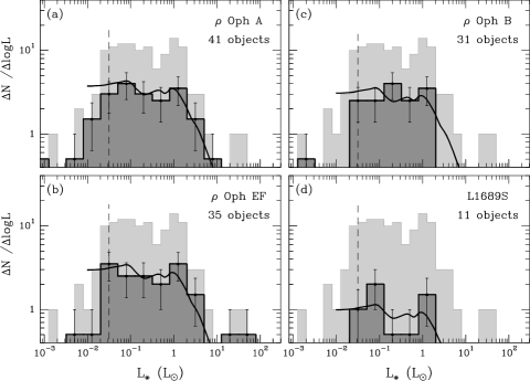
Figure 9: Individual luminosity functions for the four sub-clusters associated with the dense cores Oph A, Oph B, Oph EF, and L1689S (see Fig. 1). These are displayed with 0.4 dex bins and scaled by a factor 1/2 for direct comparison with the 0.2 dex bin total luminosity function (light grey histogram in the background). The light solid curves correspond to the model of Fig. 7a scaled to the number of stars in each sub-cluster.

6.3 Luminosity/mass functions in individual cloud cores

Our sample of Class II YSOs is large enough that we can study the properties of the four sub-clusters associated with the dense cores Oph A, Oph B, Oph EF, and L1689S (see Fig. 1). All 123 Class II sources but 5 belong to these 4 sub-clusters. The luminosity functions of Class II objects in the individual sub-clusters are displayed in Fig. 9 along with the ‘best-fit’ model of Sect. 5.1 (solid curve). They all agree reasonably well in shape with both the total luminosity function and the model: all four luminosity functions are essentially flat over two orders of magnitude in luminosity and appear to have a peak at $\mbox{$L_{\star}$}\sim 1.5\,\mbox{L${}_{\odot}$}$. The agreement is particularly good for the sub-cluster with the largest number of stars, Oph A (see Fig. 9a), but even the smallest sub-cluster, L1689S, tends to reproduce the shape of the global luminosity function on a smaller scale (Fig. 9d). In contrast, for instance, the luminosity function derived for the Chamaeleon I cloud based on ISOCAM data (Persi et al. pmo00 (2000)) differs markedly from the $\rho$ Ophiuchi luminosity functions. It does not exhibit any peak at 1.5 L_⊙ and is consistent with an older ($\sim 3$ Myr) PMS population having a similar underlying mass function (see Kaas & Bontemps kb01 (2001)).

The similarity of the individual luminosity functions suggests similar distributions of stellar ages and stellar masses in each of the four sub-clusters.

6.4 Global aspects of star formation in $\rho$ Ophiuchi

After correction for unresolved binaries (assuming a binary fraction $f=75\%$), the total number of Class II sources (including companions) down to 0.055 M_⊙ is $\sim$ 145. Assuming a Class III to Class II number ratio of 19/22 as found by X-ray surveys (Grosso et al. grosso (2000) – see Sect. 3.5), we infer the presence of $\sim 125$ Class III stars (including associated companions) in the same mass range. The typical number ratio of Class Is (plus Class 0s) to Class IIs is 18/123 suggesting an additional $\sim 21$ embedded YSOs. Altogether, we therefore estimate that there are currently $N_{\star}\sim 291$ YSOs down to $\sim 0.055\,\mbox{M${}_{\odot}$}$ including $\sim 19$ % of brown dwarfs. The average and median masses of these objects are $\sim 0.35\,\mbox{M${}_{\odot}$}$ and $\sim 0.20\,\mbox{M${}_{\odot}$}$ respectively. The total mass of condensed objects (including brown dwarfs) in the cluster is thus estimated to be $\mbox{$M_{\star}$}^{\mathrm{clust}}=291\times 0.35\sim 102\,\mbox{M${}_{\odot}$}$. (The brown dwarfs with $0.055\,\mbox{M${}_{\odot}$}<\mbox{$M_{\star}$}<0.08\,\mbox{M${}_{\odot}$}$ contribute only $\sim 4\,\%$ of this mass.) Restricting ourselves to L1688 (thus subtracting the $\sim 10\,\%$ contribution from L1689) whose average radius is approximately 0.4 pc (cf. CS contours in Fig. 1), we find $N_{\star}^{\mathrm{L1688}}\sim 262$, $\mbox{$M_{\star}$}^{\mathrm{L1688}}\sim 92\,\mbox{M${}_{\odot}$}$, $n_{\star}^{\mathrm{L1688}}\sim 980$ stars/pc³, and $\rho_{\star}^{\mathrm{L1688}}\sim 340\,\mbox{M${}_{\odot}$}$/pc³, where $n_{\star}$ and $\rho_{\star}$ are the stellar number density and stellar mass (volume) density of the cluster, respectively.

Adopting a conservative value of 2 Myr for the cluster age, the total mass of $\mbox{$M_{\star}$}^{\mathrm{clust}}=102\,\mbox{M${}_{\odot}$}$ translates into an average star formation rate of $5.1\times 10^{-5}\,\mbox{M${}_{\odot}$}/$yr, corresponding to one new YSO (of typical mass 0.20 M_⊙) every $\sim 4000$ yr.

Lastly, we can derive the star formation efficiency (SFE) in L1688, defined as SFE$=\mbox{$M_{\mathrm{star}}$}/(\mbox{$M_{\mathrm{star}}$}+\mbox{$M_{\mathrm{gas}}$})$. The total molecular gas mass, $M_{\mathrm{gas}}$, of L1688 has been estimated to range between $550\,\mbox{M${}_{\odot}$}$ (from C¹⁸O measurements – Wilking & Lada wl83 (1983)) and $1500\,\mbox{M${}_{\odot}$}$ (from CS(2-1) data – Liseau et al. liseau95 (1995)). Using $\mbox{$M_{\star}$}^{\mathrm{L1688}}=92\,\mbox{M${}_{\odot}$}$, we thus get SFE${}^{\mathrm{L1688}}\sim 6-14$ %, which is somewhat lower than previous estimates ($\geq 22\%$ – WLY89). Note, however, that active star formation in L1688 appears to be limited to the three sub-clusters/dense cores Oph A, Oph EF, and Oph B (see Fig. 1 and Loren et al. loren90 (1990)), where the local star formation efficiency is significantly higher: $SFE\sim 31\%$, using a total core mass of $200\,\mbox{M${}_{\odot}$}$ (Loren et al. loren90 (1990)).

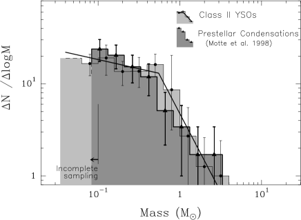
Figure 10: Comparison of the pre-stellar mass spectrum measured by MAN98 for 58 protocluster condensations (dark histogram with statistical error bars) with the YSO mass function derived in Sect. 5.1 for 123 Class II systems (light histogram with error bars accounting for both statistical and age uncertainties).

6.5 Comparison with the $\rho$ Ophiuchi protocluster condensations

In an extensive 1.3 mm dust continuum imaging survey of L1688 with the IRAM 30 m telescope (11^′′ resolution), MAN98 could identify 58 compact starless condensations. Molecular line observations (e.g. Belloche, André, & Motte bam (2001)) indicate that the condensations are gravitationally bound and thus likely pre-stellar in nature. MAN98 noted a remarkable similarity between the mass spectrum of these pre-stellar condensations and the IMF of Miller & Scalo (ms79 (1979)).

In Fig. 10, we compare the pre-stellar mass spectrum determined by MAN98 with the mass distribution of Class II YSOs derived in Sect. 5.1. (As such, both distributions are uncorrected for the presence of close binary systems.) It can be seen that there is a good agreement in shape between the two mass spectra. A Kolmogorov-Smirnov test performed on the corresponding cumulative distributions confirms that they are statistically indistinguishable at the 95% confidence level. This supports the suggestion of MAN98 that the IMF of embedded clusters is primarily determined by cloud fragmentation at the pre-stellar stage of star formation. The fact that both the pre-stellar and the YSO spectrum of Fig. 10 present a break at roughly the same mass $\sim 0.5\,\mbox{M${}_{\odot}$}$ is quite remarkable. A small, global shift of the masses by only $\sim$ 30% upward or downward in one of the spectra would make them differ at the 2$\sigma$ statistical level. Although in absolute terms, both sets of masses are probably uncertain by a factor of $\sim 2$ (due to uncertainties in the 1.3 mm dust opacity and in the cluster age, respectively), this suggests that the protocluster condensations identified at 1.3 mm may form stars/systems with an efficiency larger than $\sim$ 50–70%.

7 Conclusions

We have used ISOCAM to survey the $\rho$ Ophiuchi main cloud for embedded YSOs down to a completeness level of $\sim 10-15\,$mJy at 6.7$\,\mu$m and 14.3$\,\mu$m. Our main findings are as follows:

1. A total of 425 point sources are detected in the $\sim 0.7$ deg² field covered by the survey, of which 211 are seen at both 6.7$\,\mu$m and 14.3$\,\mu$m. The observed distribution of the flux density ratio $\mbox{$F_{\nu}^{14.3}$}/\mbox{$F_{\nu}^{6.7}$}$ is clearly bimodal with a gap separating two distinct groups of sources: a “red” group corresponding to Class I and Class II YSOs with optically thick mid-IR excesses, and a “blue” group consisting of Class III YSOs and background stars (cf. Fig. 3).

2. The red group consists of 139 cluster members, 71 of them being newly identified YSOs. Based on their mid-IR colors from 2$\,\mu$m to $6.7\,\mu$m and $14.3\,\mu$m, essentially all of these new YSOs are low-luminosity Class II objects. This brings the total number of Class II members to 123, a factor of 2 larger than previously known. Only 50 % of these Class II sources have a near-IR excess large enough to be recognizable in a near-IR color-color diagram.

3. Combining near-IR data from Barsony et al. (bklt (1997)) with our mid-IR photometry, we derive stellar luminosities for 123 Class II and 74 Class III YSOs. We also estimate bolometric luminosities for 16 Class I objects. The corresponding luminosity functions (Fig. 6) are complete down to $\sim 0.02\,\mbox{L${}_{\odot}$}$, $\sim 0.03\,\mbox{L${}_{\odot}$}$, and $\sim 0.2\,\mbox{L${}_{\odot}$}$ for Class I, Class II, and Class III objects, respectively. The luminosity function of Class II YSOs is essentially flat (in logarithmic units) below $\sim 2\,\mbox{L${}_{\odot}$}$, with a possible peak at $1.5\,\mbox{L${}_{\odot}$}$ and dip at $0.5\,\mbox{L${}_{\odot}$}$ seen in the four sub-regions Oph A, Oph B, Oph EF, and L1689S (Fig. 9).

4. The large proportion of Class II objects observed above the completeness level for Class III sources ($\mbox{$M_{\star}$}\sim 0.2\,\mbox{M${}_{\odot}$}$) suggests that more than 50% of the $\rho$ Ophiuchi embedded YSO population have optically thick circumstellar disks at mid-IR wavelengths. In a majority of cases, the luminosities of these disks are consistent with pure reprocessing of stellar light. Only $\sim 35$% of the Class II objects have excess mid-IR luminosities suggestive of substantial disk accretion rates.

5. The luminosity function of Class II objects is well modeled by a population of PMS stars with ages in the range $\sim$ 0.3$-$2 Myr and a roughly flat mass distribution below $\mbox{$M_{\mathrm{flat}}$}\sim 0.5\,\mbox{M${}_{\odot}$}$, i.e., d$N/$d log$\mbox{$M_{\star}$}\propto\mbox{$M_{\star}$}^{-0.15}$ down to $\sim 0.06\,\mbox{M${}_{\odot}$}$.

6. Pending the results of a deep X-ray census of Class III objects, we argue that the mass distribution of Class II YSOs is representative of the emergent IMF of the embedded cluster. If we account for the presence of unresolved binaries, this emergent mass function is well described by a two-segment power law with a low-mass index $\alpha_{1}=-0.35\pm 0.25$, a high-mass index $\alpha_{2}=-1.7$, and a transition mass $\mbox{$M_{\mathrm{flat}}$}=0.55\pm 0.25\,\mbox{M${}_{\odot}$}$ (where d$N/$d log$\mbox{$M_{\star}$}\propto\mbox{$M_{\star}$}^{\alpha}$). We find no evidence for a sharp turnover at low masses down to at least $\sim 0.06\,\mbox{M${}_{\odot}$}$.

7. The shape of the mass function for Class II systems is statistically indistinguishable from the mass spectrum determined at 1.3 mm by Motte, André, & Neri (man (1998)) for the pre-stellar condensations of the protocluster. This supports the conclusion of these authors that the IMF may be primarily determined by fragmentation at the pre-stellar stage of star formation. It also suggests that the 1.3 mm protocluster condensations should form stars/systems with an efficiency larger than $\sim$ 50–70%.

Table 1: List of the 212 ISOCAM sources identified as members of the $\rho$ Ophiuchi cluster

ISO Coordinates(J2000)^a $$F_{\nu}^{6.7}$$ Identification^c IR^d

# [Jy] [Jy] [Jy] [Jy] Class

1 16^h25^m368 241551 0.157 0.031 0.249 0.023 IRS2 II

2 16^h25^m382 242240 0.075 0.014 0.088 0.007 B162538242238 nII

3 16^h25^m397 242637 0.197 0.020 0.449 0.013 IRS3 nII

4 16^h25^m411 242138 0.008 0.008 - - B162541242138 III

5 16^h25^m506 243918 0.045 0.012 - - IRS10 III

6 16^h25^m563 242050 0.400 0.042 0.662 0.024 SR4/IRS12 II

7 16^h25^m575 243034 0.049 0.007 0.009 0.006 GSS20 III

8 16^h26^m015 242947 0.034 0.010 - - B162601242945 III

9 16^h26^m015 242520 0.025 0.009 0.032 0.007 SKS14 nII

10 16^h26^m032 242340 0.507 0.017 0.341 0.024 DoAr21/GSS23 III

11 16^h26^m032 241749 0.025 0.002 0.006 0.003 VSSG19 III

12 16^h26^m046 241752 0.005 0.002 0.012 0.003 B162604241753 nII

13 16^h26^m070 242728 0.112 0.022 0.128 0.015 B162607242725 nII

14 16^h26^m075 242743 0.032 0.007 - - B162607242742 III

15 16^h26^m087 241853 0.010 0.003 - - CRBR4 III?

16 16^h26^m097 243412 -^e - -^e - SR3/GSS25 III

17 16^h26^m104 242058 0.386 0.011 0.43 0.017 GSS26 II

18 16^h26^m158 241923 0.026 0.002 0.005 0.003 SKS17 III?

19 16^h26^m170 242226 0.262 0.005 0.414 0.012 GSS29 II

20 16^h26^m172 242023 0.146 0.003 0.293 0.004 DoAr24/GSS28 II

21 16^h26^m173 242349 0.246 0.004 0.363 0.004 CRBR12 nI

22 16^h26^m186 241711 0.010 0.001 - - B162618241712 III?

23 16^h26^m188 242613 0.033 0.008 0.027 0.007 SKS110 nII

24 16^h26^m189 242822 0.673 0.025 0.575 0.024 VSSG1 II

25 16^h26^m190 242307 0.051 0.008 - - CRBR17 III?

26 16^h26^m192 242416 0.056 0.006 0.074 0.004 CRBR15 nII

27 16^h26^m207 240848 0.030 0.010 0.014 0.006 WSB28 III

28 16^h26^m210 241542 0.037 0.004 0.013 0.005 B162621241544 III?

29 16^h26^m215 242307 4.09 0.12 19.1 0.26 GSS30/GY6 I

30 16^h26^m217 242602 0.028 0.007 0.033 0.014 GY5 nII

31 16^h26^m218 242249 0.066 0.013 0.119 0.025 LFAM1 I

32 16^h26^m222 244436 0.027 0.009 0.028 0.012 GY3 nII

33 16^h26^m224 242408 0.009 0.003 0.017 0.003 GY11 nII

34 16^h26^m226 242256 0.052 0.008 0.084 0.016 GY12 III

35 16^h26^m231 242849 0.018 0.008 0.026 0.014 GY15 nII

36 16^h26^m234 242102 2.59 0.068 2.56 0.066 GSS31/GY20 II

37 16^h26^m237 242440 0.395 0.005 0.405 0.007 LFAM3/GY21 II

38 16^h26^m240 244309 0.174 0.012 0.206 0.017 DoAr25/GY17 II

39 16^h26^m241 242450 2.65 0.10 2.16 0.067 S2/GY23 II

40 16^h26^m242 241614 2.73 0.027 3.02 0.030 EL24 II

41 16^h26^m253 242447 0.064 0.008 0.049 0.011 GY29 nII

42 16^h26^m277 242643 0.003 0.001 - - VSSG29/GY37 III?

43 16^h26^m280 244151 0.029 0.002 0.115 0.006 GY33 nII

44 16^h26^m285 241545 0.023 0.004 0.010 0.004 B162628241543 III?

45 16^h26^m297 241908 0.015 0.002 0.005 0.003 LFAM8/SKS119 III

46 16^h26^m305 242259 0.347 0.094 0.303 0.065 VSSG27/GY51 II

47 16^h26^m309 243107 0.012 0.008 - - IRS14/GY54 III?

48 16^h26^m342 242330 -^e - -^e - S1/GY70^f III

49 16^h26^m367 241810 0.007 0.002 - - B162636241811 III?

50 16^h26^m368 241901 0.007 0.003 - - B162636241902 III?

51 16^h26^m369 241554 0.307 0.004 0.636 0.009 B162636241554 nII

52 16^h26^m380 242301 0.057 0.049 0.066 0.059 VSSG4/GY81 nII

53 16^h26^m386 242310 0.035 0.045 0.046 0.043 GY84^g nII

54 16^h26^m406 242716 0.089 0.003 0.158 0.004 GY91/CRBR42 I

55 16^h26^m407 243053 0.004 0.002 - - IRS16/GY92 III?

56 16^h26^m41$$\aas@@fstack{s}$$6 244015 0.060 0.005 0.045 0.006 WSB37/GY93 II

57 16^h26^m418 241801 0.011 0.002 - - B162641241801 III?

58 16^h26^m420 243324 0.172 0.026 0.089 0.014 WL8/GY96 III

59 16^h26^m421 243102 0.047 0.002 0.059 0.003 WL7/GY98 II

60 16^h26^m423 242626 0.019 0.002 - - GY101 III

61 16^h26^m423 242634 0.012 0.001 - - GY103 III

62 16^h26^m429 242032 0.284 0.007 0.290 0.008 GSS37/GY110 II

63 16^h26^m431 242301 0.024 0.008 0.028 0.007 GY109 nII

64 16^h26^m438 241635 0.033 0.002 0.009 0.003 VSSG11 III

65 16^h26^m440 243448 1.27 0.043 2.57 0.029 WL12/GY111 I

66 16^h26^m443 244318 0.020 0.004 - - GY112 III

67 16^h26^m451 242310 0.291 0.013 0.307 0.012 GSS39/GY116 II

68 16^h26^m465 241203 0.352 0.006 0.240 0.004 VSS27 II

69 16^h26^m470 244430 0.011 0.002 - - GY122 III

70 16^h26^m486 242839 0.137 0.004 0.188 0.005 WL2/GY128 II

71 16^h26^m487 242628 0.006 0.002 - - GY130 III?

72 16^h26^m490 243827 0.101 0.002 0.086 0.002 WL18/GY129 II

73 16^h26^m492 242005 0.074 0.004 0.022 0.004 VSSG3/GY135 III

74 16^h26^m509 242052 0.019 0.003 - - IRS20/GY143 III?

75 16^h26^m521 243039 0.026 0.002 0.026 0.003 GY144 nII

76 16^h26^m536 243236 0.022 0.003 0.017 0.004 GY146 nII

77 16^h26^m544 242438 0.020 0.003 0.017 0.004 GY152 nII

78 16^h26^m545 242622 0.091 0.003 0.070 0.004 VSSG5/GY153 II

79 16^h26^m549 242705 0.013 0.003 0.013 0.004 GY154 nII

80 16^h26^m550 242231 0.026 0.004 0.008 0.004 GY156 III

81 16^h26^m553 242029 0.055 0.002 0.010 0.003 VSSG7/GY157 III?

82 16^h26^m567 242838 0.003 0.001 - - GY163 III?

83 16^h26^m573 241400 0.114 0.005 0.084 0.004 B162656241353 nII

84 16^h26^m574 243539 0.009 0.003 0.010 0.005 WL21/GY164 nII

85 16^h26^m583 243740 0.015 0.004 0.011 0.007 CRBR51 nII

86 16^h26^m584 242129 0.022 0.003 0.018 0.004 IRS26/GY171 nII

87 16^h26^m586 241834 0.020 0.003 0.014 0.003 B162658241836 nII

88 16^h26^m588 244537 1.41 0.090 2.29 0.17 SR24^h II

89 16^h26^m593 243557 0.004 0.002 0.008 0.005 WL14/GY172 nII

90 16^h26^m593 243501 -^e - -^e - WL22/GY174 II

91 16^h27^m018 242137 0.060 0.003 0.013 0.003 VSSG8/GY181 III?

92 16^h27^m025 243730 -^e - -^e - WL16/GY182 II

93 16^h27^m030 242616 0.026 0.003 0.021 0.004 GY188 nII

94 16^h27^m037 242007 0.008 0.002 0.007 0.003 B162703242007 nII

95 16^h27^m041 242833 0.103 0.006 0.164 0.004 WL1/GY192 II

96 16^h27^m044 244300 0.020 0.003 - - GY193 III

97 16^h27^m046 244215 0.017 0.003 - - GY194 III

98 16^h27^m046 242716 0.046 0.006 0.066 0.008 GY195 nII

99 16^h27^m054 243631 0.032 0.005 0.064 0.009 LFAM26/GY197 I

100 16^h27^m057 244012 0.007 0.002 - - B162705244013 III?

101 16^h27^m060 242619 0.025 0.002 - - IRS30/GY203 III

102 16^h27^m066 244148 0.024 0.002 0.020 0.004 GY204 nII

103 16^h27^m070 243816 0.449 0.006 0.732 0.015 WL17/GY205 II

104 16^h27^m079 244027 0.004 0.002 - - GY207 III?

105 16^h27^m092 243410 0.174 0.005 0.172 0.008 WL10/GY211 II

106 16^h27^m093 241207 0.058 0.003 0.044 0.003 B162708241204 nII

107 16^h27^m096 244025 0.079 0.002 0.096 0.004 GY213 nII

108 16^h27^m096 243721 24.0 0.66 26.2 0.50 EL29/GY214 I

109 16^h27^m096 242955 0.014 0.006 - - GY215 III?

110 16^h27^m102 241916 1.57 0.026 2.84 0.026 SR21/VSSG23 II

111 16^h27^m103 243322 0.009 0.002 - - WL9/GY220 III?

112 16^h27^m114 244046 0.221 0.006 0.391 0.010 GY224 II

113 16^h27^m117 242349 0.034 0.010 - - IRS32/GY228 III?

114 16^h27^m119 243831 0.230 0.008 0.126 0.012 WL19/GY227 II/III?

115 16^h27^m12$$\aas@@fstack{s}$$1 243448 0.024 0.003 0.019 0.006 WL11/GY229 nII

116 16^h27^m139 241825 0.074 0.005 0.073 0.005 B162713241818 nII

117 16^h27^m140 244331 0.093 0.003 0.168 0.006 GY235 nII

118 16^h27^m146 242655 0.119 0.009 0.101 0.009 IRS33/GY236 nII

119 16^h27^m154 243054 0.054 0.005 0.061 0.007 IRS35/GY238 nII

120 16^h27^m157 242646 0.167 0.010 0.152 0.014 IRS34/GY239 II

121 16^h27^m159 243846 0.151 0.004 0.782 0.010 WL20/GY240 II

122 16^h27^m161 242522 0.018 0.010 0.019 0.005 IRS36/GY241 nII

123^⋆ 16^h27^m176 240519 0.021 0.002 0.035 0.004 ISO1627176240519 nII

124 16^h27^m176 242858 0.286 0.011 0.347 0.009 IRS37/GY244 II

125 16^h27^m180 242855 0.186 0.014 0.049 0.017 WL5/GY246 III

126 16^h27^m180 242431 0.028 0.004 - - GY248 III

127 16^h27^m185 243915 0.075 0.004 0.096 0.009 GY245 II

128 16^h27^m186 242907 0.284 0.019 0.272 0.012 WL4/GY247 II

129 16^h27^m193 242845 0.285 0.015 0.218 0.006 WL3/GY249 II

130 16^h27^m195 244143 0.053 0.004 - - SR12/GY250 III

131 16^h27^m216 242152 0.014 0.004 - - GY255 III?

132 16^h27^m217 244142 2.68 0.096 2.13 0.057 IRS42/GY252 II

133 16^h27^m218 244334 0.035 0.002 0.008 0.004 GY253 III

134 16^h27^m218 242955 1.09 0.029 1.26 0.033 WL6/GY254 I

135 16^h27^m229 241800 0.049 0.003 0.011 0.003 VSSG22 III

136 16^h27^m243 244146 0.008 0.002 - - GY258 III?

137 16^h27^m248 244103 0.177 0.006 0.362 0.015 CRBR85 I

138 16^h27^m260 241928 0.006 0.002 0.006 0.002 B162726241925 nII

139 16^h27^m262 244245 0.032 0.003 0.039 0.006 GY260 nII

140 16^h27^m268 243922 0.160 0.005 0.197 0.019 GY262 II

141 16^h27^m271 244051 2.21 0.019 4.43 0.091 IRS43/GY265 I

142 16^h27^m275 243118 0.095 0.004 0.098 0.011 VSSG25/GY267 II

143 16^h27^m283 243933 4.19 0.14 11.4 0.12 IRS44/GY269 I

144 16^h27^m284 242721 0.407 0.016 0.481 0.018 IRS45/GY273 II

145 16^h27^m297 243916 0.294 0.004 0.649 0.011 IRS46/GY274 I

146 16^h27^m297 243336 0.013 0.002 - - GY278 III?

147 16^h27^m301 242743 1.78 0.017 1.54 0.017 IRS47/GY279 II

148 16^h27^m308 243404 0.014 0.002 - - GY283 III?

149 16^h27^m309 244725 0.029 0.002 0.012 0.006 B162730244726 III

150^⋆ 16^h27^m309 242734 0.078 0.008 0.094 0.007 ISO1627309242734 nII

151 16^h27^m310 242500 0.059 0.007 0.098 0.008 GY284 nII

152 16^h27^m325 243322 0.030 0.002 0.018 0.004 GY289 III

153 16^h27^m326 243242 0.020 0.003 - - GY290 III?

154 16^h27^m328 243234 0.058 0.002 0.061 0.006 GY291 nII

155 16^h27^m332 244115 0.391 0.006 0.534 0.013 GY292 II

156 16^h27^m352 243831 0.017 0.002 - - GY295 III?

157 16^h27^m356 244531 0.010 0.002 - - GY296 III

158 16^h27^m363 242834 0.006 0.003 - - GY297 III?

159 16^h27^m372 243034 5.87 0.11 6.49 0.099 IRS48/GY304 I

160 16^h27^m374 241758 0.011 0.002 0.010 0.003 B162737241756 nII

161 16^h27^m376 244240 0.071 0.003 0.161 0.008 GY301 nII

162 16^h27^m380 242525 0.005 0.003 - - GY309 III?

163 16^h27^m384 243658 0.303 0.006 0.332 0.010 IRS49/GY308 II

164 16^h27^m388 243839 0.020 0.002 0.039 0.006 GY310 nII

165 16^h27^m391 244021 0.049 0.002 0.077 0.008 GY312 nII

166 16^h27^m395 243916 0.266 0.005 0.411 0.008 GY314 II

167 16^h27^m400 244313 0.924 0.016 1.06 0.014 IRS51/GY315 I

168 16^h27^m405 242207 0.464 0.009 0.449 0.007 SR9/IRS52 II

169 16^h27^m415 243537 0.024 0.002 - - GY322 III?

170 16^h27^m418 244645 0.026 0.002 0.043 0.006 B162741244645 nII

171 16^h27^m419 244337 0.050 0.002 0.058 0.005 GY323 nII

172 16^h27^m427 243849 0.021 0.004 0.013 0.007 GY326 nII

173 16^h27^m437 244307 0.027 0.003 - - IRS53/GY334 III?

174 16^h27^m45$$\aas@@fstack{s}$$9 243800 0.003 0.002 - - GY346 III?

175 16^h27^m460 244452 0.061 0.002 0.082 0.004 GY344 nII

176 16^h27^m462 243140 0.024 0.003 0.022 0.005 GY350 nII

177 16^h27^m472 244533 0.047 0.003 0.037 0.007 GY352 nII

178 16^h27^m499 242525 0.055 0.005 0.041 0.005 GY371 nII

179 16^h27^m500 244415 0.009 0.002 - - GY370 III?

180 16^h27^m502 242543 0.182 0.005 0.045 0.006 VSSG14/GY372 III

181 16^h27^m503 243901 0.004 0.002 - - GY373 III?

182 16^h27^m517 243146 4.65 0.094 5.3 0.11 IRS54/GY378 I

183 16^h27^m519 244628 0.015 0.002 - - GY377 III

184 16^h27^m520 244048 0.067 0.002 0.017 0.004 IRS55/GY380 III

185 16^h27^m550 242839 0.025 0.002 0.026 0.002 GY397 nII

186 16^h27^m555 244449 0.011 0.002 - - GY398 III?

187 16^h27^m559 242622 0.102 0.003 0.101 0.004 SR10/GY400 II

188 16^h27^m577 244001 0.017 0.001 - - GY410 III

189 16^h27^m578 243601 0.004 0.003 - - GY412 III?

190 16^h28^m038 243443 0.009 0.001 0.012 0.003 GY450 nII

191 16^h28^m049 243452 0.036 0.002 0.012 0.003 GY463 III?

192 16^h28^m055 243355 0.002 0.001 - - GY472 III?

193 16^h28^m122 241137 0.018 0.003 0.025 0.004 B162812241138 nII

194 16^h28^m137 243248 0.052 0.001 0.040 0.002 B162813243249 nII

195^⋆ 16^h28^m168 240519 0.102 0.004 0.065 0.004 ISO1628168240519 nII

196 16^h28^m168 243704 0.108 0.002 0.128 0.002 WSB60 II

197 16^h28^m221 244249 0.017 0.001 0.010 0.002 B162821244246 nII

198 16^h28^m332 242246 0.701 0.020 0.265 0.004 SR20 III

199 16^h28^m456 242822 0.315 0.004 0.230 0.006 SR13 II

200^⋆ 16^h31^m434 245524 0.170 0.003 0.430 0.006 ISO1631434245524 nII

201^⋆ 16^h31^m487 245432 0.016 0.002 0.011 0.004 ISO1631487245432 nII

202^⋆ 16^h31^m518 245726 0.003 0.001 0.011 0.005 ISO1631518245726 nII

203^⋆ 16^h31^m520 245536 0.080 0.002 0.322 0.004 ISO1631520245536 nII

204 16^h31^m520 245618 1.19 0.011 1.84 0.016 L1689IRS5 II

205^⋆ 16^h31^m531 245504 0.073 0.001 0.076 0.002 ISO1631531245504 nII

206^⋆ 16^h31^m548 250350 0.055 0.002 0.045 0.004 ISO1631548250350 nII

207 16^h31^m552 250324 0.355 0.005 0.582 0.006 IRAS162892457 nII

208^⋆ 16^h31^m591 245442 0.023 0.002 0.026 0.002 ISO1631591245442 nII

209 16^h32^m010 245644 0.982 0.019 1.17 0.011 IRS67/L1689IRS6 I

210^⋆ 16^h32^m021 245616 0.012 0.003 0.031 0.003 ISO1632021245616 nII

211^⋆ 16^h32^m056 250234 0.019 0.002 0.031 0.003 ISO1632056250234 nII

212 16^h32^m212 243035 0.489 0.005 0.807 0.004 L1689IRS7 II

• The absolute ISOCAM coordinates have been determined using the Barsony et al. (bklt (1997)) database as a reference frame. The resulting positional uncertainty is estimated to be $\sim 3\arcsec$ (rms).

• The quoted rms uncertainties on $F_{\nu}^{6.7}$ and $F_{\nu}^{14.3}$ comprise the random errors estimated from the temporal and spatial noises measured on the data. They do not include the systematic errors due to absolute calibration and aperture correction uncertainties. The maximum systematic error is estimated to be less than $\sim 15\,$%.

• For a more complete cross-identification of the $\rho$ Ophiuchi IR sources, see, e.g., Table 1 of AM94 and Table 3 of Barsony et al. (bklt (1997)). “B” refers to Barsony et al. (bklt (1997)). “ISO” refers to the present survey. Twelve ISO sources are completely new sources with respect to published IR surveys; they are named after their ISOCAM coordinates and marked by a ^⋆.

• Adopted SED classes for the ISOCAM sources (see text in Sect. 3). “nI” and “nII” indicate newly identified Class I and Class II YSOs; a question mark indicates an uncertain classification.

• ISO16$\,=\,$SR3, ISO48$\,=\,$S1, ISO90$\,=\,$WL22, and ISO92$\,=\,$WL16 are extended sources in the mid-IR range, most probably due to PAH-like emission. No attempt has been made to estimate their integrated $F_{\nu}^{6.7}$ and $F_{\nu}^{14.3}$ fluxes.

• No precise mid-IR position could be derived for ISO48$\,=\,$S1/GY70. The quoted coordinates correspond to the near-IR position of Barsony et al. (bklt (1997)).

• The position of ISO53 is offset by $\sim 16\arcsec$ to the south of the near-IR source GY84. This large mid-IR offset is most likely due to the presence of extended, structured emission from the bright neighboring source S1.

• ISO88$\,=\,$SR24 is a binary system (SR24S/GY167 and SR24N/GY168; e.g. Greene et al. gwayl (1994)) which is not resolved in the ISOCAM images.

Table 2: Class I YSOs

ISO Identification $$\alpha_{\mathrm{IR}}^{2-14}$$ ^b

#^a [L_⊙]

182 IRS54/GY378 1.76 6.6

143 IRS44/GY269 1.57 8.7

137 CRBR85 1.48 0.36

99 LFAM26/GY197 1.25 0.064

29 GSS30/GY6 1.20 21.

31 LFAM1 1.08 0.13

65 WL12/GY111 1.04 2.6

108 EL29/GY214 0.98 26.

141 IRS43/GY265 0.98 6.7

145 IRS46/GY274 0.94 0.62

21 CRBR12 0.91 0.42

209 IRS67/L1689IRS6 0.74 1.5

54 GY91/CRBR42 0.70 0.17

134 WL6/GY254 0.59 1.7

159 IRS48/GY304^c 0.18 7.4

167 IRS51/GY315^c 0.04 1.1

• The ISO number refers to the numbering of Table 1(available only in electronic form at http://cdsweb.u-strasbg.fr/).

• $L_{\mathrm{bol}}$ is estimated by integrating under the observed SED from 1.2$\,\mu$m to 60$\,\mu$m or 100$\,\mu$m and extrapolating from 60$\,\mu$m or 100$\,\mu$m to 200$\,\mu$m with a spectral index of $\mbox{$\alpha_{\mathrm{IR}}$}=-1.0$. For the 9 weak sources (ISO # 137, 99, 31, 65, 146, 21, 209, 54 and 133) without reliable IRAS fluxes, $L_{\mathrm{bol}}$ is estimated using a typical $\mbox{$L_{\mathrm{bol}}$}/\mbox{$L_{\mathrm{cal}}$}(6.7-14.3\mu$m) ratio of 9.8 (see Sect. 4.3).

• Although ISO159$\,=\,$IRS48 and ISO167$\,=\,$IRS51 formally lie below our practical Class I$-$Class II limit ($\mbox{$\alpha_{\mathrm{IR}}^{2-14}$}=0.55$), they are still considered as Class I YSOs here (cf. WLY89 and AM94).

Table 3: Class II YSOs

ISO Identification $$\alpha_{\mathrm{IR}}^{2-14}$$

#^a [mag] [mag] [mag] [L_⊙] [L_⊙]

170 B162741244645 0.51 - 6.1 24.9 0.018 0.047

103 WL17/GY205 0.42 5.2 - 22.5 0.12 0.76

124 IRS37/GY244 0.35 - 2.4 36.9 0.99 0.50

112 GY224 0.34 - 2.4 36.2 1.1 0.56

118 IRS33/GY236 0.32 - 3.6 38.3 0.28 0.15

33 GY11 0.31 10.1 - 2.7 0.001 0.010

119 IRS35/GY238 0.30 - 3.4 45.7 0.34 0.11

129 WL3/GY249 0.23 - 2.2 42.2 1.3 0.34

75 GY144 0.20 - 5.9 26.8 0.023 0.030

147 IRS47/GY279 0.17 2.6 - 26.8 1.9 1.8

46 VSSG27/GY51 0.17 5.2 - 21.6 0.11 0.30

127 GY245 0.17 6.7^b - 24.7 0.023 0.11

161 GY301 0.12 - 2.1 44.9 1.5 0.25

132 IRS42/GY252 0.08 2.1 - 27.7 3.1 2.5

77 GY152 0.05 - - - 0.037^c 0.015

70 WL2/GY128 0.05 - 2.3 38.6 1.1 0.27

165 GY312 0.03 6.6 - 14.8 0.027 0.064

85 CRBR51 0.03 - - - 0.025^c 0.010

175 GY344 0.02 6.5 - 17.4 0.030 0.074

26 CRBR15 0.01 6.7 - 14.6 0.022 0.061

139 GY260 0.03 - 3.7 40.3 0.24 0.058

37 LFAM3/GY21 0.06 4.5 - 14.5 0.25 0.33

121 WL20/GY240 0.07 3.3 - 16.5 0.86 0.67

51 B162636241554 0.09 4.4 - 7.6 0.28 0.43

95 WL1/GY192 0.11 4.9 - 20.9 0.15 0.16

122 IRS36/GY241 0.11 - 4.9 34.3 0.066 0.025

171 GY323 $$-$$0.12 - 4.0 30.9 0.19 0.070

107 GY213 0.15 5.6 - 19.4 0.075 0.089

76 GY146 0.16 - 4.1 43.5 0.17 0.025

120 IRS34/GY239 0.23 - 2.4 34.8 1.1 0.19

144 IRS45/GY273 0.24 3.6 - 19.5 0.66 0.45

204 L1689IRS5^d 0.25 2.6 - 12.8 1.9 1.4

17 GSS26 0.30 3.2 - 22.6 0.95 0.43

93 GY188 0.36 6.3 - 20.5 0.034 0.020

98 GY195 0.36 5.5 - 20.6 0.087 0.063

53 GY84 0.39 5.8 - 14.1 0.060 0.037

190 GY450 0.39 9.2 - 8.6 0.002 0.008

23 SKS110 0.41 7.2 - 8.2 0.013 0.018

13 B162607242725 0.41 4.6 - 19.5 0.22 0.12

117 GY235 0.43 4.9 - 9.9 0.16 0.12

212 L1689IRS7^d 0.44 2.6 - 14.7 1.8 0.64

79 GY154 0.44 - 5.5 24.3 0.033 0.013

24 VSSG1 0.49 3.2 - 17.1 0.97 0.49

3 IRS3 0.50 4.3 - 4.6 0.31 0.28

39 S2/GY23 0.51 2.0 - 11.8 3.7 1.6

140 GY262 0.52 3.5 - 23.7 0.71 0.20

40 EL24 0.54 1.8 - 10.0 4.5 2.1

52 VSSG4/GY81 0.54 5.2 - 17.6 0.11 0.058

154 GY291 0.60 4.3 - 23.0 0.29 0.058

94 B162703242007 0.61 - 6.6 16.6 0.010 0.006

128 WL4/GY247 0.67 3.2 - 19.5 1.1 0.24

59 WL7/GY98 0.69 4.1 - 27.2 0.37 0.061

84 WL21/GY164 0.70 7.8 - 14.2 0.007 0.008

67 GSS39/GY116 0.72 3.1 - 16.3 1.1 0.25

41 GY29 0.73 5.1 - 19.1 0.13 0.043

88 SR24N/GY168 0.74 2.5 - 7.7 2.1 0.76

35 GY15 0.75 6.2 - 11.5 0.040 0.019

164 GY310 0.75 6.4 - 4.0 0.032 0.024

63 GY109 0.77 5.8 - 14.6 0.064 0.022

151 GY284 0.77 4.9 - 7.6 0.15 0.065

43 GY33 0.78 4.2 - 15.5 0.36 0.092

138 B162726241925 0.78 7.9 - 11.2 0.006 0.004

36 GSS31/GY20 0.79 1.5 - 6.1 5.9 1.6

177 GY352 0.79 5.2 - 17.7 0.11 0.031

197 B162821244246 0.81 6.0 - 20.3 0.050 0.009

110 SR21/VSSG23 0.81 1.9 - 3.5 4.0 1.7

166 GY314 0.83 3.4 - 6.4 0.80 0.26

9 SKS14 0.85 6.0 - 9.5 0.051 0.022

12 B162604241753 0.86 6.6 - 13.4 0.027 0.009

155 GY292 0.90 2.7 - 10.8 1.6 0.37

88 SR24S/GY167 0.91 2.5 - 5.9 2.2 0.72

19 GSS29 0.91 2.9 - 9.4 1.4 0.28

115 WL11/GY229 0.92 6.3 - 13.8 0.037 0.015

196 WSB60^e 0.92 4.9 - 2.8 0.16 0.075

30 GY5 0.92 6.3 - 2.5 0.036 0.019

176 GY350 0.94 6.4 - 6.4 0.033 0.014

72 WL18/GY129 0.94 4.7 - 10.4 0.19 0.061

163 IRS49/GY309 0.96 3.1 - 10.1 1.1 0.23

193 B162812241138 0.99 6.2 - 6.2 0.039 0.016

2 B162538242238 1.00 4.6 - 10.9 0.22 0.063

78 VSSG5/GY153 1.02 3.8 - 19.7 0.55 0.056

86 IRS26/GY171 1.04 5.2 - 19.9 0.12 0.015

105 WL10/GY211 1.05 3.4 - 12.5 0.78 0.12

87 B162658241836 1.06 6.0 - 14.2 0.050 0.011

160 B162737241756 1.08 7.2 - 4.5 0.014 0.006

83 B162656241353 1.08 4.2 - 11.1 0.33 0.058

32 GY3 $$-$$1.09 6.5 - 0.4 0.029 0.015

1 IRS2 1.09 3.4 - 4.9 0.79 0.15

185 GY397 1.10 6.1 - 4.1 0.045 0.016

6 SR4/IRS12 1.12 2.8 - 1.9 1.5 0.37

142 VSSG25/GY267 1.13 4.0 - 9.8 0.42 0.065

20 DoAr24/GSS28 1.14 3.5 - 1.8 0.72 0.16

178 GY371 1.16 5.2 - 7.1 0.11 0.026

62 GSS37/GY110 1.19 2.7 - 8.5 1.6 0.18

89 WL14/GY172 1.24 5.8 - 17.2 0.059 0.006

194 B162813243249 1.24 5.2 - 5.9 0.12 0.024

116 B162713241818 1.27 3.7 - 10.7 0.57 0.046

106 B162708241204 1.33 4.5 - 8.0 0.24 0.027

102 GY204 1.33 6.2 - 1.5 0.039 0.011

168 SR9/IRS52 1.35 2.7 - 0.7 1.6 0.23

199 SR13 1.37 3.4 - 0.9 0.78 0.12

187 SR10/GY400 1.39 4.1 - 3.2 0.38 0.052

68 VSS27 1.53 2.6 - 5.6 1.9 0.13

172 GY326 1.56 5.3 - 8.5 0.11 0.008

56 WSB37/GY93 1.58 4.7 - 1.2 0.20 0.024

38 DoAr25/GY17 1.58 3.4 - 0.7 0.83 0.11

- GY256 - - 4.5 34.5 0.11 -

- GY257 - - 4.1 33.2 0.17 -

90 WL22/GY174 - - - - 29.^f -

92 WL16/GY182 - - - - 44.^f -

207 IRAS162892457 - - - - 1.3^c 0.51

123 New^g - - - - 0.077^c 0.031

150 New^g - - - - 0.21^c 0.083

195 New^g - - - - 0.14^c 0.058

200 New^g - - - - 0.95^c 0.38

201 New^g - - - - 0.025^c 0.010

202 New^g - - - - 0.024^c 0.010

203 New^g - - - - 0.71^c 0.28

205 New^g - - - - 0.17^c 0.067

206 New^g - - - - 0.099^c 0.040

208 New^g - - - - 0.058^c 0.023

210 New^g - - - - 0.067^c 0.027

211 New^g - - - - 0.068^c 0.027

The sample of 21 Class II sources with $-0.05\leq\mbox{$\alpha_{\mathrm{IR}}^{2-14}$}\leq 0.55$ might contain a significant population of transition objects (flat-spectrum objects) between Class I protostars and Class II T Tauri stars.

• The ISO number refers to the numbering in Table 1 (available only in electronic form at http://cdsweb.u-strasbg.fr/).

• The J-band flux of ISO127$\,=\,$GY245 is taken from Greene et al. (gwayl (1994)).

• ISO77$\,=\,$GY152, ISO85$\,=\,$CRBR51, and the last 13 sources are not detected in all near-IR bands, and no reliable $M_{J}$ or $M_{H}$ can be estimated. $L_{\star}$ has been obtained using Eq. 8 (Sect. 4.2).

• ISO204$\,=\,$L1689-IRS5 and ISO212$\,=\,$L1689-IRS7 refer to the IR sources listed by Greene et al. (gwayl (1994)) in L1689.

• ISO196$\,=\,$WSB60 corresponds to the source B162816$-$243657 in Barsony et al. (bklt (1997)).

• Since ISO90$\,=\,$WL22 and ISO92$\,=\,$WL16 are young early-type stars (see Sect. 3.1), $L_{\star}$ cannot be derived accurately using the method described in Sect. 4.1. The quoted luminosities for WL22 and WL16 are taken from WLY89 and Comerón et al. (crbr (1993)), respectively. They have been scaled to $d=140\,$pc.

• The adopted names and the J2000 coordinates of the completely new IR sources are given in Table 1.

Table 4: Class III YSOs

ISO Identification $$\alpha_{\mathrm{IR}}^{2-14}$$

#^a () [mag] [mag] [mag] [L_⊙]

114 WL19/GY227^b 0.05 - 1.0 73.4 52.

125 WL5/GY246^b 1.02 - 0.7 59.8 39.

34 GY12^b 1.06 3.3 - 19.5 0.89

58 WL8/GY96^b 1.11 1.9 - 35.5 4.2

152 GY289^b 1.33 3.3 - 27.5 0.90

198 SR20 1.65 1.9 - 4.0 4.0

133 GY253^b 1.73 3.3 - 31.2 0.85

45 LFAM8/SKS119^b 1.82 4.2 - 25.2 0.34

80 GY156^b 2.00 3.4 - 22.5 0.84

10 DoAr21/GSS23^b 2.00 0.7 - 6.0 15.

27 WSB28 2.06 4.1 - 4.3 0.36

149 B162730244726 2.20 3.7 - 10.3 0.61

135 VSSG22 2.23 3.0 - 17.1 1.2

64 VSSG11^b 2.24 3.4 - 15.2 0.83

73 VSSG3/GY135 2.26 2.3 - 15.7 2.8

180 VSSG14/GY372 2.51 2.2 - 5.5 3.0

184 IRS55/GY380 2.65 2.6 - 6.0 1.8

11 VSSG19^b 2.75 3.8 - 3.9 0.50

7 GSS20 2.84 3.1 - 4.7 1.1

60 GY101^b ( 0.00) - 2.0 55.5 2.0

61 GY103^b (0.45) - 2.6 48.5 1.1

126 GY248^b (0.82) 4.2 - 25.5 0.36

101 IRS30/GY203^b (0.99) - 2.2 36.5 1.6

14 B162607242742 (1.43) 3.5 - 20.6 0.70

8 B162601242945 (1.96) 3.9 - 8.1 0.47

183 GY377^b (1.98) 4.0 - 16.0 0.40

157 GY296^b (2.02) 5.5 - 5.1 0.081

4 B162541242138 (2.05) 5.8 - 6.7 0.060

69 GY122 (2.17) 5.5 - 2.7 0.080

96 GY193 (2.24) 4.2 - 7.4 0.34

97 GY194 (2.35) 4.1 - 9.1 0.40

188 GY410 (2.36) 4.0 - 10.2 0.43

66 GY112 (2.42) 4.2 - 3.6 0.35

130 SR12/GY250^b (2.48) 3.4 - 1.2 0.83

5 IRS10 (2.78) 2.7 - 5.4 1.7

- IRS50/GY306 3.7 - 11.5 0.60

16 SR3/GSS25 - - - 100.^c

48 S1/GY70^b - - - 1100.^c

• The ISO number refers to the numbering in Table 1 (available only in electronic form at http://cdsweb.u-strasbg.fr/).

• Class III YSOs located inside the CS contours of Fig. 1 (see Sect. 3.5 and 4.4).

• For the two B stars ISO16$\,=\,$SR3 and ISO48$\,=\,$S1 (e.g. Elias elias (1978)), $L_{\star}$ cannot be derived using the method described in Sect. 4.1. The quoted values are taken from Lada & Wilking (lw84 (1984)), and have been scaled to $d=140\,$pc.

Table 5: Class III candidates located within the CS contours of Fig. 1

ISO Identification $$\alpha_{\mathrm{IR}}^{2-14}$$

#^a () [mag] [mag] [mag] [L_⊙]

191 GY463 1.46 4.4 - 25.2 0.28

44 B162628241543 1.63 3.9 - 21.7 0.45

81 VSSG7/GY157 2.13 2.1 - 29.8 3.4

91 VSSG8/GY181 2.20 2.4 - 22.9 2.4

28 B162621241544 2.23 2.9 - 15.5 1.4

18 SKS17 2.38 3.6 - 17.4 0.64

25 CRBR17 ( 0.68) 8.3 - 10.1 0.004

153 GY290 ( 0.41) - 3.7 41.5 0.31

100 B162705244013^b ( 0.12) - - - -

109 GY215^b ( 0.05) - - - -

104 GY207 (0.31) - 4.6 39.5 0.11

49 B162636241811^b (0.36) - - - -

15 CRBR4 (0.41) - 1.9 58.9 2.2

146 GY278 (0.58) - 2.4 47.8 1.3

136 GY258 (0.72) 8.2 - 10.8 0.004

55 IRS16/GY92 (0.80) - 5.0 29.1 0.079

173 IRS53/GY334 (0.81) - 2.0 40.2 2.1

71 GY130 (0.87) - 3.7 38.8 0.31

162 GY309 (1.01) - 3.3 42.5 0.47

50 B162636241902 (1.06) 6.6 - 14.0 0.025

57 B162641241801 (1.22) - 3.1 32.3 0.58

111 WL9/GY220 (1.27) 5.5 - 21.6 0.086

22 B162618241712 (1.50) 4.2 - 26.8 0.34

113 IRS32/GY228 (1.52) 3.6 - 18.5 0.62

82 GY163 (1.53) - 4.1 32.8 0.19

131 GY255 (1.57) 4.2 - 21.6 0.35

169 GY322 (1.59) 4.0 - 16.3 0.43

47 IRS14/GY54 (1.85) 4.7 - 16.6 0.21

189 GY412 (1.90) 5.2 - 17.6 0.12

181 GY373 (1.91) 6.4 - 7.7 0.032

174 GY346 (1.93) 5.6 - 19.5 0.075

74 IRS20/GY143 (1.97) 3.8 - 16.0 0.50

179 GY370 (1.99) 5.4 - 10.0 0.094

148 GY283 (2.09) 4.3 - 13.1 0.32

42 VSSG29/GY37 (2.14) 6.8 - 6.5 0.021

192 GY472 (2.14) 5.9 - 20.1 0.054

186 GY398 (2.20) 5.2 - 5.2 0.11

158 GY297 (2.22) 6.0 - 0.7 0.047

156 GY295 (2.52) 4.3 - 4.8 0.32

• The ISO number refers to the numbering in Table 1 (available only in electronic form at http://cdsweb.u-strasbg.fr/).

• $A_{V}$ and $L_{\star}$ were not derived for these sources as they were detected only in the K band by Barsony et al. (bklt (1997)).