Relativistic approach to positronium levels in a strong magnetic field

Abstract

We have investigated the bound states of an electron and positron in superstrong magnetic fields typical for neutron stars. The complete relativistic problem of positronium in a strong magnetic field has not been succesfully solved up to now. In particular, we have studied the positronium when it moves relativistically across the magnetic field. A number of problems which deal with the pulsar magnetosphere, as well as the evolution of protoneutron stars, could be considered as a field for application.

I Introduction

Theoretical models for radio-pulsar emission mechanisms include the bound states of a relativistic electron and positron in a superstrong magnetic field. The year 1985 was marked by a number of papers, where the authors tried to take into account the positronium contribution into the dispersion equation of a photon which propagates in a superstrong magnetic field (Leinson & Oraevsky, [1], [2]); Herold et al.,[3]; Shabad & Usov, [4]). Nevertheless, the correct solution of the completely relativistic problem for the bound states of an electron and positron in a superstrong magnetic field remains unknown. Koller et al. [5] have formulated the quadratic form of the completely relativistic Dirac equation for bound states of an electron and positron in a magnetic field of arbitrary intensity. However, they only found a solution for the simplest case, when positronium does not move across the magnetic field. There was also the work of Shabad and Usov [6], where they tried to solve the Bethe-Salpeter equation for a positronium atom relativistically moving across the superstrong magnetic field. Unfortunately, they did not take into account the retardation effect in the interaction between the electron and positron. For this reason, we return to the problem of positronium in a superstrong magnetic field. We suggest a solution of the Bethe-Salpeter equation for positronium relativistically propagating across the superstrong magnetic field. The results which contradict those given by Shabad and Usov are discussed.

This paper is organized as follows. In Section 2 we state the problem by considering the Bethe-Salpeter equation for a bound electron-positron pair interacting with an external magnetic field. The problem can be simplified when the adiabatic approximation (discussed in Section 3) holds, since in this case only one Landau level for each particle has to be taken into account. In section 4, we concentrate on the particular case when the electron and positron occupy the same Landau level. As a particularly important case, we devote Sect. 5 to the ground band of positronium levels, and analyze some particular cases. In Appendix A we recall the explicit formulae of the electron (or positron) wave function in the presence of an external magnetic field.

II Bethe-Salpeter equation for a bound pair of electron and positron in a strong magnetic field

To find the bound states of electron and positron in a strong magnetic field, we start from the Bethe-Salpeter equation for the scattering amplitude, to the lowest order in the fine structure’s constant $e^{2}\simeq 1/137$

$$\Gamma_{i_{j}}\left(p_{-},-p_{+}\right)=ie^{2}\int\frac{d^{3}{\bf p}_{-}^{{}^{\prime}}}{\left(2\pi\right)^{3}}\frac{d^{3}{\bf p}_{+}^{{}^{\prime}}}{\left(2\pi\right)^{3}}\frac{d^{4}q}{\left(2\pi\right)^{4}}G_{il}\left(p_{-},p_{-}^{{}^{\prime}}\right)\gamma_{ls}^{\mu}\Gamma_{st}(p_{-}^{{}^{\prime}}-q,-p_{+}^{{}^{\prime}}-q)\gamma_{tq}^{\nu}G_{qj}\left(-p_{+}^{{}^{\prime}},-p_{+}\right)D_{\mu\nu}\left(q\right)$$ (1)

where $\widehat{G}\left(p_{-},p_{-}^{{}^{\prime}}\right)$ and $\widehat{G}\left(-p_{+}^{\prime},-p_{+}\right)$ are the propagators of the electron and positron, respectively, in an external uniform magnetic field, which will be taken as directed along the $Z$ axis. Here and henceforth, a $-$ ($+$) subscript denotes the electron (positron), and summation over repeated indices will be understood. $D_{\mu\nu}\left(q\right)$ , with $q=(\omega,{\bf q)}$ is the photon propagator. In Eq. (1) $p_{-},p_{+},q,p_{+}^{{}^{\prime}}$ and $p_{-}^{{}^{\prime}}$ are the four-momenta of the interacting particles.

It is convenient to study this equation in the mixed (coordinates-energy) representation. To this purpose, we define the new unknown function

$$\chi_{ij}\left({\bf r}_{-},{\bf r}_{+};{\bf\varepsilon}_{-},{\bf-\varepsilon}_{+}\right)\equiv\int\frac{d^{3}{\bf p}_{-}}{\left(2\pi\right)^{3}}\frac{d^{3}{\bf p}_{+}}{\left(2\pi\right)^{3}}{\bf\exp\ }\left(i{\bf p}_{-}{\bf r}_{-}\right)\Gamma_{ij}(p_{-},-p_{+}){\bf\exp\ }\left(i{\bf p}_{+}{\bf r}_{+}\right).$$ (2)

which depend on both individual space coordinates ${\bf r}_{\mp}$ and energies of the electron and the positron. Their energies can be written as:

$${\bf\varepsilon}_{-}=\frac{E}{2}+\varepsilon,\hskip 72.26999pt{\bf\varepsilon}_{+}=\frac{E}{2}-\varepsilon$$ (3)

where the total energy $E$ of the bound pair is an integral of motion in the stationary state we are considering. By the use of Fourier transformation of the Green’s functions

$$\widehat{G}\left(p_{-},p_{-}^{{}^{\prime}}\right)=\int d^{3}{\bf r}_{-}^{{}^{\prime}}d^{3}{\bf r}_{-}\widehat{G}({\bf r}_{-}{\bf,r}_{-}^{{}^{\prime}}{\bf\ ;\varepsilon}_{-}{\bf)\exp\ }[-i{\bf p}_{-}{\bf r}_{-}+i{\bf p}_{-}^{\prime}{\bf r}_{-}^{\prime}]$$ (4)

$$\widehat{G}\left(-p_{+}^{\prime},-p_{+}\right)=\int d^{3}{\bf r}_{+}^{{}^{\prime}}d^{3}{\bf r}_{+}\widehat{G}({\bf r}_{+}^{\prime}{\bf,r}_{+}{\bf\ ;-\varepsilon}_{+}{\bf)\exp\ }[i{\bf p}_{+}^{\prime}{\bf r}_{+}^{\prime}-i{\bf p}_{+}{\bf r}_{+}]$$ (5)

we obtain the following equation:

$$\chi_{ij}\left({\bf r}_{-},{\bf r}_{+};\frac{E}{2}+\varepsilon,{\bf-}\frac{E}{2}+\varepsilon\right)=ie^{2}\int d^{3}{\bf r}_{-}^{{}^{\prime}}d^{3}{\bf r}_{+}^{{}^{\prime}}G_{il}({\bf r}_{-}{\bf,r}_{-}^{{}^{\prime}}{\bf;}\frac{E}{2}+\varepsilon{\bf)}G_{qj}({\bf r}_{+}^{\prime}{\bf,r}_{+}{\bf;-}\frac{E}{2}+\varepsilon{\bf)}$$ (6)

$$\times\int\frac{d^{3}{\bf q}d\omega}{\left(2\pi\right)^{4}}D_{\mu\nu}\left({\bf\ \omega,q}\right){\bf\exp\ }\left[i{\bf q}\left({\bf r}_{-}^{\prime}-{\bf r}_{+}^{\prime}\right)\right]\gamma_{ls}^{\mu}\chi_{st}\left({\bf r}_{-}^{\prime},{\bf r}_{+}^{\prime};\frac{E}{2}+\varepsilon-\omega,{\bf-}\frac{E}{2}+\varepsilon-\omega\right)\gamma_{tq}^{\nu}$$ (7)

We choose the following gauge :

$$A_{0}=0,{\bf A}=(0,Bx,0)$$ (8)

so that $B_{x}=B_{y}=0$, $B_{z}=B$. In this way, the Green’s function of the electron takes the general form :

$$G({\bf r}_{-}{\bf,r}_{-}^{{}^{\prime}}{\bf;}\varepsilon_{-}{\bf)}=\sum_{n\sigma}\int\frac{dk_{3}^{-}}{2\pi}\frac{dk_{2}^{-}}{2\pi}\exp[ik_{3}^{-}(z_{-}-z_{-}^{{}^{\prime}})+ik_{2}^{-}(y_{-}-y_{-}^{{}^{\prime}})]\frac{\Psi_{n\sigma}^{\left(+\right)}(x_{-}+\frac{k_{2}^{-}}{eB},k_{3}^{-})\overline{\Psi}_{n\sigma}^{(+)}(x_{-}^{{}^{\prime}}+\frac{k_{2}^{-}}{eB},k_{3}^{-})}{[\varepsilon_{-}-E_{n}(k_{3}^{-})+i0]},$$ (9)

where $E_{n}(k_{3}^{-})=\sqrt{m_{n}^{2}+\left(k_{3}^{-}\right)^{2}}$ and $m_{n}\equiv m\sqrt{1+2nb}$, with $b\equiv B/B_{0}.$ ($B_{0}=m^{2}/e=4.4\times 10^{13}G$ is the so-called critical magnetic field). The electron wave functions $\Psi_{n\sigma}^{\left(+\right)}$ are bispinors of positive frequency which correspond to Landau states of the electron in the magnetic field. Each Landau state of the electron is marked by the number $n=0,1,...$ which characterizes the quantized motion across the magnetic field; $k_{3\text{ }}^{-}$ is the electron momentum along the magnetic field; $\sigma=\pm 1$ corresponds to the spin projection of the electron $s_{3}=\pm 1/2$. For many applications, it is convenient to use wave functions of negative frequency for the states of positron (See Appendix A). Then, the positron propagator has the following form:

$$G({\bf r}_{+}^{{}^{\prime}}{\bf,r}_{+}{\bf;}\varepsilon_{+}{\bf)}=\sum_{n^{\prime}\sigma}\int\frac{dk_{3}^{+}}{2\pi}\frac{dk_{2}^{+}}{2\pi}\exp[-ik_{3}^{+}(z_{+}^{{}^{\prime}}-z_{+})-ik_{2}^{+}(y_{+}^{{}^{\prime}}-y_{+})]\frac{\Psi_{n^{\prime}\sigma}^{\left(-\right)}(x_{+}^{{}^{\prime}}-\frac{k_{2}^{+}}{eB},-k_{3}^{+})\overline{\Psi}_{n^{\prime}\sigma}^{(-)}(x_{+}-\frac{k_{2}^{+}}{eB},-k_{3}^{+})}{[\varepsilon_{+}+E_{n^{\prime}}(k_{3}^{+})-i0]}{},$$ (10)

where $E_{n^{\prime}}(k_{3}^{+})=\sqrt{m_{n^{\prime}}^{2}+\left(k_{3}^{+}\right)^{2}}$. We assume that the center of mass of the positronium can move relativistically in any direction with respect to the magnetic field, i.e., we make no assumption about the center of mass momentum

$$P_{3}=k_{3}^{-}+k_{3}^{+}$$ (11)

along the magnetic field, but we assume that the longitudinal relative motion of the electron and positron is nonrelativistic. Therefore, the relative momentum projection

$$k_{3}=\frac{m_{n^{{}^{\prime}}}k_{3}^{-}-m_{n}k_{3}^{+}}{m_{n}+m_{n^{{}^{\prime}}}}$$ (12)

is much smaller than the electron mass. Let us write the electron and positron momenta in the following form :

$$k_{3}^{-}=\frac{m_{n}}{m_{n}+m_{n^{{}^{\prime}}}}P_{3}+k_{3}$$ (13)

$$k_{3}^{+}=\frac{m_{n^{\prime}}}{m_{n}+m_{n^{{}^{\prime}}}}P_{3}-k_{3}$$ (14)

Thus, we may expand the Landau levels energy as a series of $k_{3}$ :

$$E_{n}(k_{3}^{-})\simeq\frac{m_{n}\sqrt{M_{nn^{\prime}}^{2}+P_{3}^{2}}}{M_{nn^{\prime}}}+\frac{P_{3}k_{3}}{\sqrt{M_{nn^{\prime}}^{2}+P_{3}^{2}}}+\frac{M_{nn^{\prime}}^{3}}{\left(M_{nn^{\prime}}^{2}+P_{3}^{2}\right)^{3/2}}\frac{k_{3}^{2}}{2m_{n}}$$ (15)

$$E_{n^{\prime}}(k_{3}^{+})\simeq\frac{m_{n^{\prime}}\sqrt{M_{nn^{\prime}}^{2}+P_{3}^{2}}}{M_{nn^{\prime}}}-\frac{P_{3}k_{3}}{\sqrt{M_{nn^{\prime}}^{2}+P_{3}^{2}}}+\frac{M_{nn^{\prime}}^{3}}{\left(M_{nn^{\prime}}^{2}+P_{3}^{2}\right)^{3/2}}\frac{k_{3}^{2}}{2m_{n^{\prime}}}$$ (16)

where $M_{nn^{\prime}}\equiv m_{n}+m_{n^{{}^{\prime}}}$. This yields

$$E_{n}(k_{3}^{-})+E_{n^{\prime}}(k_{3}^{+})\simeq\sqrt{M_{nn^{\prime}}^{2}+P_{3}^{2}}+\frac{k_{3}^{2}}{2\mu_{nn^{\prime}}}$$ (17)

with the reduced mass

$$\mu_{nn^{\prime}}=\frac{m_{n}m_{n^{\prime}}}{M_{nn^{\prime}}}\frac{\left(M_{nn^{\prime}}^{2}+P_{3}^{2}\right)^{3/2}}{M_{nn^{\prime}}^{3}}$$ (18)

III Adiabatic approximation

In a sufficiently strong magnetic field $B>>10^{9}G$ the Larmor radius

$$a_{L}=\frac{1}{\sqrt{eB}}$$ (19)

is small with respect to the Bohr’s radius

$$a_{B}=\frac{1}{me^{2}}$$ (20)

because :

$$\frac{a_{B}}{a_{L}}=\sqrt{eB}\frac{1}{me^{2}}=\frac{\sqrt{b}}{e^{2}}>>1.$$ (21)

When inequality (21) holds, the Coulomb’s binding energy $|\varepsilon|\sim me^{4}$ is much smaller than the distance between Landau levels of the electron (or positron). This means that the energies $\varepsilon_{\mp}$ of the bound electron and positron vary in a small vicinity of the Landau levels they occupy. In this case, the poles near these Landau levels give the principal contribution to the Green’s functions of the electron and the positron. Therefore, we can write :

$$\hat{G}^{n}({\bf r}_{-}{\bf,r}_{-}^{{}^{\prime}}{\bf;}\varepsilon_{-}{\bf)}=\sum_{\sigma}\int\frac{dk_{3}^{-}}{2\pi}\frac{dk_{2}^{-}}{2\pi}\exp[ik_{3}^{-}(z_{-}-z_{-}^{{}^{\prime}})+ik_{2}^{-}(y_{-}-y_{-}^{{}^{\prime}})]\frac{\Psi_{n\sigma}^{\left(+\right)}(x_{-}+\frac{k_{2}^{-}}{eB},k_{3}^{-})\overline{\Psi}_{n\sigma}^{(+)}(x_{-}^{{}^{\prime}}+\frac{k_{2}^{-}}{eB},k_{3}^{-})}{[\varepsilon_{-}-E_{n}(k_{3}^{-})+i0]}$$ (22)

$$\hat{G}^{n^{\prime}}({\bf r}_{+}^{{}^{\prime}}{\bf,r}_{+}{\bf;\varepsilon}_{+}{\bf)}=\sum_{\sigma}\int\frac{dk_{3}^{+}}{2\pi}\frac{dk_{2}^{+}}{2\pi}\exp[-ik_{3}^{+}(z_{+}^{{}^{\prime}}-z_{+})-ik_{2}^{+}(y_{+}^{{}^{\prime}}-y_{+})]\frac{\Psi_{n^{\prime}\sigma}^{\left(-\right)}(x_{+}^{{}^{\prime}}-\frac{k_{2}^{+}}{eB},-k_{3}^{+})\overline{\Psi}_{n^{\prime}\sigma}^{(-)}(x_{+}-\frac{k_{2}^{+}}{eB},-k_{3}^{+})}{[\varepsilon_{+}+E_{n^{\prime}}(k_{3}^{+})-i0]}{}$$ (23)

Generally speaking, in the case of $n\neq n^{\prime}$ two terms corresponding to the same total energy $E=\varepsilon_{+}+\varepsilon_{-}$ give the major contribution to the product of Green functions in the right-hand side of the Bethe-Salpeter equation. The first of them corresponds to an electron occupying the Landau level  $n$, while the positron occupies the level $n^{{}^{\prime}}$. The second term is the state with the same energy, but with the electron occupying the level $n^{{}^{\prime}}$ and the positron in the state $n$. Within this adiabatic approximation, it is possible to characterize the positronium states in a strong magnetic field by the almost-good quantum numbers $n$ and $n^{{}^{\prime}}$ , and by other additional constants, which characterize the motion of the center of mass and the relative motion of the electron and positron along the magnetic field .

IV Equation for the bound state wave function for equal Landau numbers

If both the electron and the positron occupy the same Landau level, then virtual photons with small values of $\omega\sim me^{4}\ll\left|{\bf q}\right|\sim me^{2}$ give the major contribution to the $e^{+}e^{-}$ interaction. Therefore, we can neglect $\omega$ in the photon propagator

$$D_{\mu\nu}\left({\bf\ \omega,q}\right)=g_{\mu\nu}\frac{4\pi}{\omega^{2}-{\bf q}^{2}}\simeq-g_{\mu\nu}\frac{4\pi}{{\bf q}^{2}}$$ (24)

This yields, for $n=n^{\prime}$:

$$\chi_{ij}\left({\bf r}_{-},{\bf r}_{+};\frac{E}{2}+\varepsilon,{\bf-}\frac{E}{2}+\varepsilon\right)=-ie^{2}\int d^{3}r_{-}^{{}^{\prime}}d^{3}r_{+}^{{}^{\prime}}G_{il}^{n}({\bf r}_{-}{\bf,r}_{-}^{{}^{\prime}}{\bf;}\frac{E}{2}+\varepsilon{\bf)}G_{qj}^{n}({\bf r}_{+}^{\prime}{\bf,r}_{+}{\bf;-}\frac{E}{2}+\varepsilon{\bf)}$$ (25)

$${\bf\times}\int\frac{d^{3}q}{\left(2\pi\right)^{3}}\frac{4\pi}{{\bf q}^{2}}{\bf\exp\ }\left[i{\bf q}\left({\bf r}_{-}^{\prime}-{\bf r}_{+}^{\prime}\right)\right]g_{\mu\nu}\gamma_{ls}^{\mu}\int\frac{d\omega}{2\pi}\chi_{st}\left({\bf r}_{-}^{\prime},{\bf r}_{+}^{\prime};\frac{E}{2}+\omega,{\bf-}\frac{E}{2}+\omega\right)\gamma_{tq}^{\nu}$$ (26)

By performing integration over $d\varepsilon/2\pi$, we obtain the wave function of the bound pair

$$\hat{\Phi}({\bf r}_{-},{\bf r}_{+};E)=\int\frac{d\varepsilon}{2\pi}\chi_{ij}\left({\bf r}_{-},{\bf r}_{+};\frac{E}{2}+\varepsilon,{\bf\ -}\frac{E}{2}+\varepsilon\right)$$ (27)

which verifies the following equation:

$$\hat{\Phi}\left({\bf r}_{-},{\bf r}_{+};E\right)=-ie^{2}\int\frac{d^{3}r_{-}^{{}^{\prime}}d^{3}r_{+}^{{}^{\prime}}}{\left|{\bf r}_{-}^{\prime}-{\bf r}_{+}^{\prime}\right|}\frac{d\varepsilon}{2\pi}\hat{G}^{n}({\bf r}_{-}{\bf,r}_{-}^{{}^{\prime}}{\bf;}\frac{E}{2}+\varepsilon{\bf)}\gamma^{\mu}\hat{\Phi}\left({\bf r}_{-}^{\prime},{\bf r}_{+}^{\prime};E\right)\gamma_{\mu}\hat{G}^{n}({\bf r}_{+}^{\prime}{\bf,r}_{+}{\bf;-}\frac{E}{2}+\varepsilon{\bf)}$$ (28)

Integration over $d\varepsilon^{{}^{\prime}}/2\pi$ in the right-hand side can be done with the help of the following formula :

$$\int_{-\infty}^{\infty}\frac{d\varepsilon}{2\pi}\frac{1}{\left(\varepsilon+E/2-E_{n}(k_{3}^{-})+i0\right)\left(\varepsilon-E/2+E_{n^{\prime}}(k_{3}^{+})-i0\right)}=\frac{i}{E-E_{n}(k_{3}^{-})-E_{n^{\prime}}(k_{3}^{+})}$$ (29)

Thus, one has

$$Q_{ilqj}^{nn^{\prime}} \equiv \int\frac{d\varepsilon^{{}^{\prime}}}{2\pi}G_{il}^{n}({\bf r}_{-}{\bf,r}_{-}^{{}^{\prime}}{\bf;}\frac{E}{2}+{\bf\varepsilon}^{{}^{\prime}}{\bf)}G_{qj}^{n^{\prime}}({\bf r}_{+}{\bf,r}_{+}^{{}^{\prime}}{\bf;-}\frac{E}{2}+{\bf\varepsilon}^{{}^{\prime}}{\bf)}=\sum_{\sigma}\sum_{\sigma^{{}^{\prime}}}i\int\frac{dk_{3}^{-}}{2\pi}\frac{dk_{2}^{-}}{2\pi}\frac{dk_{3}^{+}}{2\pi}\frac{dk_{2}^{+}}{2\pi}$$ (32)

$$\times{}\frac{\exp[ik_{3}^{-}(z_{-}-z_{-}^{{}^{{}^{\prime}}})+ik_{2}^{-}(y_{-}-y_{-}^{{}^{\prime}})-ik_{3}^{+}(z_{+}^{{}^{\prime}}-z_{+})-ik_{2}^{+}(y_{+}^{{}^{\prime}}-y_{+})]}{E-E_{n}(k_{3}^{-})-E_{n^{\prime}}(k_{3}^{+})}{}$$

$$\ \ \times\Psi_{n\sigma}^{i\left(+\right)}(x_{-}+\frac{k_{2}^{-}}{eB})\overline{\Psi}_{n\sigma}^{l(+)}(x_{-}^{{}^{\prime}}+\frac{k_{2}^{-}}{eB})\Psi_{n^{{}^{\prime}}\sigma^{{}^{\prime}}}^{q\left(-\right)}(x_{+}^{{}^{\prime}}-\frac{k_{2}^{+}}{eB})\overline{\Psi}_{n^{{}^{\prime}}\sigma^{{}^{\prime}}}^{j(-)}(x_{+}-\frac{k_{2}^{+}}{eB})$$

Since the relative motion of the bound pair along the magnetic field is nonrelativistic, we neglect $k_{3}^{\pm\text{ }}\sim me^{2}$ inside the bispinors. The Landau level energies of the electron and positron are given by Eqs. (15,16).

Let us introduce the new coordinates :

$$Z = \frac{m_{n}z_{-}+m_{n^{{}^{\prime}}}z_{+}}{m_{n}+m_{n^{{}^{\prime}}}},\qquad Y=\frac{1}{2}(y_{-}+y_{+}),\qquad X=\frac{1}{2}(x_{-}+x_{+})$$ (33)

$$z = z_{-}-z_{+},\qquad y=y_{-}-y_{+},\qquad x=x_{-}-x_{+}$$ (34)

$$Z_{1} = \frac{m_{n}z_{-}^{{}^{\prime}}+m_{n^{{}^{\prime}}}z_{+}^{{}^{\prime}}}{m_{n}+m_{n^{{}^{\prime}}}},\qquad Y_{1}=\frac{1}{2}(y_{-}^{{}^{\prime}}+y_{+}^{{}^{\prime}}),\qquad X_{1}=\frac{1}{2}(x_{-}^{{}^{\prime}}+x_{+}^{{}^{\prime}})$$ (35)

$$z_{1} = z_{-}^{{}^{\prime}}-z_{+}^{{}^{\prime}},\qquad y_{1}=y_{-}^{{}^{\prime}}-y_{+}^{{}^{\prime}},\qquad x_{1}=x_{-}^{{}^{\prime}}-x_{+}^{{}^{\prime}}$$ (36)

and new momenta :

$$P_{3} = k_{3}^{-}+k_{3}^{+},\qquad P_{2}=k_{2}^{-}+k_{2}^{+}$$ (37)

$$k_{3} = \frac{m_{n^{{}^{\prime}}}k_{3}^{-}-m_{n}k_{3}^{+}}{m_{n}+m_{n^{{}^{\prime}}}},\qquad k_{2}=\frac{1}{2}(k_{2}^{-}-k_{2}^{+})$$ (38)

The expression for $Q_{nn^{\prime}}$ reads now :

$$Q_{ilqj}^{nn^{\prime}} = i\int\frac{dP_{3}}{2\pi}\frac{dk_{3}}{2\pi}\frac{dP_{2}}{2\pi}\frac{dk_{2}}{2\pi}\frac{\exp\{iP_{3}(Z-Z_{1})+iP_{2}(Y-Y_{1})+ik_{3}(z-z_{1})+ik_{2}(y-y_{1})\}}{\varepsilon-\frac{k_{3}^{2}}{2\mu_{nn^{\prime}}}-\frac{P_{3}^{2}}{2M_{nn^{{}^{\prime}}}}}$$ (41)

$$\times\sum_{\sigma}\sum_{\sigma^{{}^{\prime}}}\Psi_{n\sigma}^{i\left(+\right)}(X+\frac{x}{2}+\frac{P_{2}+2k_{2}}{2eB})\overline{\Psi}_{n\sigma}^{l(+)}(X_{1}+\frac{x_{1}}{2}+\frac{P_{2}+2k_{2}}{2eB})$$

$$\times\Psi_{n^{{}^{\prime}}\sigma^{{}^{\prime}}}^{q\left(-\right)}(X_{1}-\frac{x_{1}}{2}-\frac{P_{2}-2k_{2}}{2eB})\overline{\Psi}_{n^{{}^{\prime}}\sigma^{{}^{\prime}}}^{j(-)}(X-\frac{x}{2}-\frac{P_{2}-2k_{2}}{2eB})$$

and the positronium wave function obeys the following equation:

$$\hat{\Phi}\left({\bf r},{\bf R};E\right)= e^{2}\int\frac{dZ_{1}dY_{1}dX_{1}d^{3}r_{1}}{r_{1}}\frac{dP_{3}}{2\pi}\frac{dk_{3}}{2\pi}\frac{dP_{2}}{2\pi}\frac{dk_{2}}{2\pi}\frac{\exp\{iP_{3}(Z-Z_{1})+iP_{2}(Y-Y_{1})\}}{\varepsilon-\frac{k_{3}^{2}}{2\mu_{nn^{\prime}}}-\frac{P_{3}^{2}}{2M_{nn^{{}^{\prime}}}}}\exp\{ik_{3}(z-z_{1})+ik_{2}(y-y_{1})\}$$ (44)

$$\times\sum_{\sigma}\sum_{\sigma^{{}^{\prime}}}\Psi_{n\sigma}^{i\left(+\right)}(X+\frac{x}{2}+\frac{P_{2}+2k_{2}}{2eB})\overline{\Psi}_{n\sigma}^{l(+)}(X_{1}+\frac{x_{1}}{2}+\frac{P_{2}+2k_{2}}{2eB})$$

$$\times\gamma^{\mu}\hat{\Phi}\left({\bf r}_{1},{\bf R}_{1};E\right)\gamma_{\mu}\Psi_{n\sigma^{\prime}}^{q\left(-\right)}(X_{1}-\frac{x_{1}}{2}-\frac{P_{2}-2k_{2}}{2eB})\overline{\Psi}_{n\sigma^{\prime}}^{j(-)}(X-\frac{x}{2}-\frac{P_{2}-2k_{2}}{2eB}).$$

To separate the motion of the center of mass we subtract a bilocal phase (Avron et al., [7])

$${\bf PR+}e{\bf rA}({\bf R)}$$ (45)

from $\hat{\Phi}$, with the help of the gauge choice Eq. (8). Thus, one has

$$\hat{\Phi}({\bf r}_{-},{\bf r}_{+};E)={}\exp[iP_{3}^{0}Z+iP_{2}^{0}Y-ieBXy]\hat{\phi}({\bf r})$$ (46)

By using this expression one can perform the integration on the right-hand side of Eq. (44) over $dZ_{1}dY_{1}$. Thus, we obtain the $\delta$- functions $\delta(P_{3}-P_{3}^{0})\delta(P_{2}-P_{2}^{0})$, which allow for integration over $dP_{3}dP_{2}$. Therefore, we will substitute everywhere the constants of motion $P_{3}^{0},P_{2}^{0}$ instead of $P_{3}$ and $P_{2}$ . We consider the reference frame $P_{3}^{0}=0$. Thus, the equation for the stationary states becomes the following:

$$\hat{\phi}({\bf r})= e^{2}\int\frac{d^{3}r_{1}}{r_{1}}\frac{dk_{3}}{2\pi}\frac{1}{\varepsilon-\frac{k_{3}^{2}}{2\mu_{nn^{\prime}}}}\int\frac{dk_{2}}{2\pi}\exp\left(ik_{2}y+ieBXy\right)\int dX_{1}\exp\left(-ik_{2}y_{1}-ieBX_{1}y_{1}\right)\exp\{ik_{3}(z-z_{1})\}$$ (49)

$$\times\sum_{\sigma}\sum_{\sigma^{{}^{\prime}}}\Psi_{n\sigma}^{\left(+\right)}(X+\frac{x}{2}+\frac{P_{2}^{0}+2k_{2}}{2eB})\overline{\Psi}_{n\sigma}^{(+)}(X_{1}+\frac{x_{1}}{2}+\frac{P_{2}^{0}+2k_{2}}{2eB})$$

$$\times\gamma^{\mu}\hat{\phi}({\bf r}_{1})\gamma_{\mu}\Psi_{n\sigma^{\prime}}^{\left(-\right)}(X_{1}-\frac{x_{1}}{2}-\frac{P_{2}^{0}-2k_{2}}{2eB})\overline{\Psi}_{n\sigma^{\prime}}^{(-)}(X-\frac{x}{2}-\frac{P_{2}^{0}-2k_{2}}{2eB})$$

The right-hand side of Eq.(49) depends on $z$ only through the exponential ${}\exp(ik_{3}z)$. The action of the operator

$$\widehat{H}_{z}^{0}\equiv-\frac{1}{2\mu_{nn^{{}^{\prime}}}}\frac{\partial^{2}}{\ \partial z^{2}}-\varepsilon\text{.}$$ (50)

on Eq.(49) cancels the denominator on the right-hand side. Subsequent integration over $dk_{3}$ yields $\delta(z-z_{1})$, and integration over $dz_{1}$ becomes trivial. Finally, we obtain :

$$\widehat{H}_{z}^{0}\hat{\phi}({\bf r}) = -e^{2}\int\frac{dx_{1}dy_{1}}{\sqrt{x_{1}^{2}+y_{1}^{2}+z^{2}}}\int\frac{dk_{2}}{2\pi}\exp\left(ik_{2}y+ieBXy\right)\int dX_{1}\exp\left(-ik_{2}y_{1}-ieBX_{1}y_{1}\right)$$ (53)

$$\times\sum_{\sigma}\sum_{\sigma^{{}^{\prime}}}\Psi_{n\sigma}^{\left(+\right)}(X+\frac{x}{2}+\frac{P_{2}^{0}+2k_{2}}{2eB})\overline{\Psi}_{n\sigma}^{(+)}(X_{1}+\frac{x_{1}}{2}+\frac{P_{2}^{0}+2k_{2}}{2eB})$$

$$\times\gamma^{\mu}\hat{\phi}({\bf r}_{1})\gamma_{\mu}\Psi_{n\sigma^{\prime}}^{\left(-\right)}(X_{1}-\frac{x_{1}}{2}-\frac{P_{2}^{0}-2k_{2}}{2eB})\overline{\Psi}_{n\sigma^{\prime}}^{(-)}(X-\frac{x}{2}-\frac{P_{2}^{0}-2k_{2}}{2eB})$$

Let us now introduce the new integration variables

$$\xi=X+\frac{k_{2}}{eB},\qquad\lambda=X_{1}+\frac{k_{2}}{eB}$$ (54)

and denote by $x_{0}$ the distance between the orbiting centers of the electron and positron in the plane orthogonal to the magnetic field:

$$x_{0}\equiv\frac{P_{2}^{0}}{eB}$$ (55)

This distance depends on the transverse momentum $P_{2}^{0}$, which characterizes the motion of the mass center across the magnetic field. Then

$$\widehat{H}_{z}^{0}\hat{\phi}(x,y,z)=-e^{2}eB\sum_{\sigma}\sum_{\sigma^{{}^{\prime}}}\int\frac{d\xi}{2\pi}{}\exp(ieB\xi y)\Psi_{n\sigma}^{\left(+\right)}(\xi+\frac{x+x_{0}}{2})\overline{\Psi}_{n\sigma^{\prime}}^{(-)}(\xi-\frac{x+x_{0}}{2})$$ (56)

$$\times\int\frac{dx_{1}dy_{1}}{\sqrt{x_{1}^{2}+y_{1}^{2}+z^{2}}}\int d\lambda{}\exp(-ieB\lambda y_{1}){}\overline{\Psi}_{n\sigma}^{(+)}(\lambda+\frac{x_{1}+x_{0}}{2})\gamma^{\mu}\hat{\phi}(x_{1},y_{1},z)\gamma_{\mu}\Psi_{n\sigma^{\prime}}^{\left(-\right)}(\lambda-\frac{x_{1}+x_{0}}{2})$$ (57)

As follows from the last equation, the wave function describing the relative motion has the form :

$$\hat{\phi}({\bf r})=\sum_{\sigma}\sum_{\sigma^{{}^{\prime}}}f_{\sigma\sigma^{\prime}}^{n}(z)\int\frac{d\xi}{2\pi}{}\exp\left(ieB\xi y\right)\Psi_{n\sigma}^{\left(+\right)}(\xi+\frac{x+x_{0}}{2})\overline{\Psi}_{n\sigma^{{}^{\prime}}}^{(-)}(\xi-\frac{x+x_{0}}{2})$$ (58)

where the functions $f_{\sigma\sigma^{\prime}}^{n}$ depend only on the relative coordinate $z$. These functions are solutions of the following set of Schrödinger-like equations:

$$-\frac{1}{2\mu_{nn}}\frac{\partial^{2}}{\partial z^{2}}f_{\sigma\sigma^{\prime}}^{n}(z,x_{0})+\sum_{\kappa\kappa^{\prime}}V_{\sigma\sigma^{\prime}}^{\kappa\kappa^{\prime}}(z,x_{0})f_{\kappa\kappa^{\prime}}^{n}(z,x_{0})=\varepsilon f_{\sigma\sigma^{\prime}}^{n}(z,x_{0})$$ (59)

Here, the effective potentials represent the Coulomb interaction, averaged over the fast transverse motion of the interacting particles :

$$V_{\sigma\sigma^{\prime}}^{\kappa\kappa^{\prime}}(z) \equiv -e^{2}\frac{eB}{2\pi}\int\frac{dxdyd\xi d\lambda{}\exp\left[ieB\left(\xi-\lambda\right)y\right]{}}{\sqrt{\left(x-x_{0}\right)^{2}+y^{2}+z^{2}}}$$ (61)

$$\times Tr\left[{}\overline{\Psi}_{n\sigma}^{(+)}(\lambda+\frac{x}{2})\gamma^{\mu}\Psi_{n\kappa}^{\left(+\right)}(\xi+\frac{x}{2})\right]\left[\overline{\Psi}_{n\kappa^{{}^{\prime}}}^{(-)}(\xi-\frac{x}{2})\gamma_{\mu}\Psi_{n\sigma^{\prime}}^{\left(-\right)}(\lambda-\frac{x}{2})\right]$$

In general, the matrix $V_{\sigma\sigma^{\prime}}^{\kappa\kappa^{\prime}}(z)$ consists on 16 elements corresponding to different spin orientations of the two particles. However, in the adiabatic approximation, most of them are zero. After integration over $d\lambda d\xi$, we obtain the effective potentials in the following form:

$$V_{\sigma\sigma^{\prime}}^{\kappa\kappa^{\prime}}(z)=-\frac{e^{3}B}{2\pi}\int\int\frac{dxdy{}\exp(-\rho^{2}/2)}{\sqrt{(x-x_{0})^{2}+y^{2}+z^{2}}}R_{\sigma\sigma^{\prime}}^{\kappa\kappa^{\prime}}(x,y)$$ (62)

where

$$\ R_{\sigma\sigma^{\prime}}^{\kappa\kappa^{\prime}}(x,y)\equiv\exp\left(\rho^{2}/2\right)\int\frac{d\xi d\lambda}{2\pi}{}\exp\left[ieB(\xi-\lambda)y\right]$$ (63)

$$\times\left[{}\overline{\Psi}_{n\sigma}^{(+)}(\lambda+\frac{x}{2})\gamma^{\mu}\Psi_{n\kappa}^{\left(+\right)}(\xi+\frac{x}{2})\right]\left[\overline{\Psi}_{n\kappa^{{}^{\prime}}}^{(-)}(\xi-\frac{x}{2})\gamma_{\mu}\Psi_{n\sigma^{\prime}}^{\left(-\right)}(\lambda-\frac{x}{2})\right]$$ (64)

with $\rho=\sqrt{eB\left(x^{2}+y^{2}\right)}$.

V The ground band of positronium states in a superstrong magnetic field.

The lowest band of positronium levels corresponds to the case when both the electron and the positron occupy the ground Landau level with $n=n^{\prime}=0$. Only a spin combination, spin-down for the electron and spin-up for the positron, is possible in this case. A simple calculation, using the wave functions of Appendix A, gives the following result:

$$R_{\uparrow\uparrow}^{\uparrow\uparrow}(x,y)=R_{\downarrow\downarrow}^{\downarrow\downarrow}(x,y)=R_{\uparrow\uparrow}^{\downarrow\downarrow}(x,y)=R_{\downarrow\downarrow}^{\uparrow\uparrow}(x,y)=-R_{\uparrow\downarrow}^{\downarrow\uparrow}(x,y)=-R_{\downarrow\uparrow}^{\uparrow\downarrow}(x,y)=R_{\uparrow\downarrow}^{\uparrow\downarrow}(x,y)=0$$ (65)

and

$$R_{\downarrow\uparrow}^{\downarrow\uparrow}(x,y)=1.$$ (66)

Consequently, the wave functions of the lowest band, which will be labeled by the quantum number $l$, have the following form :

$$\hat{\phi}_{00l}^{P_{2}^{0}}({\bf r})=f_{\downarrow\uparrow}^{(0,l)}(z,x_{0})\int\frac{d\xi}{2\pi}{}\exp(ieB\xi y)\Psi_{0\downarrow}^{\left(+\right)}(\xi+\frac{x+x_{0}}{2})\overline{\Psi}_{0\uparrow}^{(-)}(\xi-\frac{x+x_{0}}{2})$$ (67)

Using the formulae for bispinors corresponding to Landau states (see Appendix A), we can integrate this expression over $d\xi$. The result is :

$$\hat{\phi}_{00l}^{P_{2}^{0}}({\bf r})=f_{\downarrow\uparrow}^{(0,l)}(z,x_{0})\sqrt{\frac{eB}{2\pi}}{}\exp\{-\frac{eB}{4}[(x+x_{0})^{2}+y^{2}]\}\left(\begin{tabular}[]{l}$0$\\ $1$\\ $0$\\ $0$\end{tabular}\right)\left(\begin{array}[]{cccc}0&0&0&1\end{array}\right)$$ (68)

The wave function for the relative motion along the magnetic field can be found by solving the following Schrödinger equation :

$$-\frac{1}{2\mu_{00}}\frac{\partial^{2}}{\partial z^{2}}f_{\downarrow\uparrow}^{(0,l)}(z,x_{0})+V_{\downarrow\uparrow}^{\downarrow\uparrow}(z,x_{0})f_{\downarrow\uparrow}^{(0,l)}(z,x_{0})=\varepsilon_{00}^{l}\left(x_{0}\right)f_{\downarrow\uparrow}^{(0,l)}(z,x_{0})$$ (69)

with $\mu_{00}=m/2$. The effective potential is

$$V_{00}(z,x_{0})\equiv V_{\downarrow\uparrow}^{\downarrow\uparrow}(z,x_{0})=-\frac{2e^{2}}{\pi}\int_{0}^{\infty}\frac{\rho d\rho{}\exp(-\rho^{2}/2)}{\sqrt{(\rho a_{L}-x_{0})^{2}+z^{2}}}\ {\sf K}\left(i\sqrt{\frac{4\rho x_{0}a_{L}}{(\rho a_{L}-x_{0})^{2}+z^{2}}}\right)$$ (70)

and

$${\sf K}\left(k\right)=\int_{0}^{\pi/2}\frac{d\theta}{\sqrt{1-k^{2}\sin^{2}\theta}}$$ (71)

is the elliptic integral of the first kind.

Eq. (70) depends on the parameter $x_{0}=P_{2}^{0}/eB$, therefore the eigen-functions $f_{\downarrow\uparrow}^{(0,l)}$, as well as the discrete spectrum eigen-energies $\varepsilon_{00}^{l}$, depend on the quantity $P_{2}^{0}$ , which characterizes the relativistic motion of the center of mass across the magnetic field. Unfortunately the integration in Eq. (70) can not be done analytically. By this reason, we consider several limiting cases.

A The case of small $x_{0}$ .

We first consider the case of a small distance between the centers of Landau orbits in the plane orthogonal to the magnetic field:

$$\sqrt{eB}x_{0}=\frac{P_{2}^{0}}{\sqrt{eB}}\ll 1$$ (72)

This yields:

$$V_{00}(z)\approx-e^{2}\sqrt{\frac{\pi eB}{2}}\left[1-{}\mathop{\rm erf}\left(|z|\sqrt{\frac{eB}{2}}\right)\right]{}\exp\left(\frac{eBz^{2}}{2}\right)$$ (73)

with

$$\mathop{\rm erf}(x)=\frac{2}{\sqrt{\pi}}\int_{0}^{x}dt\exp\left(-t^{2}\right)$$ (74)

being the error function. At distances $\left|z\right|\gg a_{L}$, the potential behaves as the one-dimensional Coulomb potential

$$V_{00}(z)\approx-\frac{e^{2}}{\left|z\right|}$$ (75)

while for $\left|z\right|\ll a_{L}$ goes to a constant

$$V_{00}(0)=-\sqrt{\frac{\pi}{2}}\frac{e^{2}}{a_{L}}$$ (76)

(This result differs from that given by Usov and Shabad by the factor $\sqrt{\pi/2}$).

For shallow levels, the characteristic size of the atom along the $Oz$ axis is of the order $a_{B}\gg a_{L\text{ }}$, so that the potential can be considered to have the form Eq. (75), and the energy levels should be close to Balmer’s spectrum. This statement is not valid for deep levels. Eq. (69), with the potential Eq. (73), can be solved numerically. However, an analytical estimate is of interest. To obtain such an estimate, we replace the potential Eq. (73) by a simple function of the form

$$V_{00}(z)\approx-\frac{e^{2}}{\left|z\right|+\sqrt{\frac{2}{\pi}}a_{L}}$$ (77)

which slightly differs from Eq. (73) only in the region $\left|z\right|\sim a_{L}$, and has the same asymptotic forms.

1 Discrete spectrum.

Solutions to the Schrödinger equation with this potential have been investigated by Loudon [8] for negative energy. For completeness, we quote shortly this calculations, which will be used later for investigation of the states of positive energy. We define, as in [8], a dimensionless quantity $\alpha$ by writing

$$\varepsilon=-\frac{1}{2\mu_{00}a_{00}^{2}\alpha^{2}}$$ (78)

with $a_{00}=\left(\mu_{00}e^{2}\right)^{-1}=2a_{B}$, and replace the independent variable $z$ in Eq. (69) by

$$z^{\prime} = \frac{2}{\alpha a_{00}}\left(\sqrt{\frac{2}{\pi}}a_{L}+z\right),\hskip 72.26999pt\text{for }z>0$$ (79)

$$z^{\prime} = -\frac{2}{\alpha a_{00}}\left(\sqrt{\frac{2}{\pi}}a_{L}-z\right),\hskip 72.26999pt\text{for }z<0$$ (80)

whereupon, for $z\neq 0$, the equation takes the Whittaker’s form of the confluent hypergeometric equation

$$\frac{d^{2}f}{dz^{\prime 2}}-\frac{1}{4}f+\frac{\alpha}{\left|z^{\prime}\right|}f=0$$ (81)

This equation has two independent solutions, given by Whittaker’s functions. The first of them

$$M_{\alpha,\frac{1}{2}}\left(z^{\prime}\right)=\exp\left(-z^{\prime}/2\right)z^{\prime}\Phi(1-\alpha,2;z^{\prime})$$ (82)

where $\Phi(1-\alpha,2;z^{\prime})$ is the confluent hypergeometric function of the first kind, diverges as $\left(z^{\prime}\right)^{-\alpha}\exp\left(z^{\prime}/2\right)$ for large $z$. Since for a bound state any solution of this equation must go to zero when $\left|z^{\prime}\right|$ tends to infinity, we choose the second solution, which for $z>0$ is

$$W_{\alpha,\frac{1}{2}}\left(z^{\prime}\right)=\exp\left(-z^{\prime}/2\right)z^{\prime}\Psi(1-\alpha,2;z^{\prime})$$ (83)

where $\Psi(1-\alpha,2;x)$ is the confluent hypergeometric function of the second kind :

$$\Psi(1-\alpha,2;x)=\frac{1}{\Gamma\left(-\alpha\right)}\{\,\Phi(1-\alpha,2;x)[\log x+\psi\left(1-\alpha\right)-\psi\left(1\right)-\psi\left(2\right)]-\frac{1}{\alpha x}+\sum_{r=1}^{\infty}\frac{\left(1-\alpha\right)_{r}}{r!\left(r+1\right)!}A_{r}x^{r}\}$$ (84)

Here

$$A_{r}=\sum_{n=0}^{r-1}\left[\frac{1}{n+1-\alpha}-\frac{1}{n+1}-\frac{1}{n+2}\right],\hskip 72.26999pt\left(c\right)_{r}=\frac{\Gamma\left(c+r\right)}{\Gamma\left(c\right)}$$ (85)

The function $\psi\left(s\right)=\Gamma^{\prime}\left(s\right)/\Gamma\left(s\right)$ is the logarithmic derivative of the gamma function. The solutions for positive and negative $z$ can be joined together to form either even or odd wave-functions. For an odd state we require

$$W_{\alpha,\frac{1}{2}}\left(\sqrt{\frac{2}{\pi}}\frac{2a_{L}}{\alpha a_{00}}\right)=0$$ (86)

while for an even state

$$\left[\frac{d}{dz^{\prime}}W_{\alpha,\frac{1}{2}}\left(z^{\prime}\right)\right]_{z^{\prime}=\sqrt{\frac{2}{\pi}}\frac{2a_{L}}{\alpha a_{00}}}=0$$ (87)

To find solutions to Eqs. (86) and (87), which give the eigenvalues of the system, we keep only terms which are dominant when

$$x=\sqrt{\frac{2}{\pi}}\frac{2a_{L}}{\alpha a_{00}}$$ (88)

is very small, and $\alpha$ is close to a positive integer. The eigenvalue conditions then become :

Odd state:

$$\psi\left(1-\alpha\right)\sqrt{\frac{2}{\pi}}\frac{2a_{L}}{\alpha a_{00}}-\frac{1}{\alpha}=0$$ (89)

Even state:

$$\log\frac{2}{\alpha a_{00}}\sqrt{\frac{2}{\pi}}a_{L}+\,\psi\left(1-\alpha\right)=0$$ (90)

Assuming $\alpha\rightarrow l$ where $l=1,2,...$ we can replace

$$\,\psi\left(1-\alpha\right)\rightarrow\frac{1}{\alpha-l}$$ (91)

Then, the quantum defects $\delta_{l}=\alpha-l$ are given by

Odd state:

$$\delta_{l}=\frac{2}{a_{00}}\sqrt{\frac{2}{\pi}}a_{L}$$ (92)

Even state:

$$\delta_{l}=-\left[\log\frac{2}{la_{00}}\sqrt{\frac{2}{\pi}}a_{L}\right]^{-1}$$ (93)

For the adiabatic case one has $\delta_{l}\ll 1$ if $\log(a_{00}/a_{L})\gg 1$.

In addition to this series of states having their quantum numbers $\alpha$ close to positive integers, there is another state having $\alpha$ close to zero. For such a value of $\alpha$, $\psi\left(1-\alpha\right)$ is no longer an important term in Eq. (90), and $1/\alpha$ becomes the dominant term in $\alpha$. In this case, the equation for the eigenvalues becomes

$$\log\frac{2}{\alpha a_{00}}\sqrt{\frac{2}{\pi}}a_{L}=-\frac{1}{2\alpha}$$ (94)

The quantum defect $\delta_{l}=\alpha$ for the state $l=0$ can be found from Eq. (94) by iteration. To the first order in $a_{L}/a_{00}$ its binding energy is given by

$$\varepsilon_{1}^{\left(0\right)}=\varepsilon_{2}^{\left(0\right)}\approx-me^{4}\left(\log\sqrt{\frac{\pi}{2}}\frac{a_{00}}{2a_{L}}\right)^{2}$$ (95)

To this state there corresponds the even wave-function

$$f_{\downarrow\uparrow}^{(0,0)}(z,0)=\left[\frac{1}{a_{00}}\ln\left(\sqrt{\frac{\pi}{2}}\frac{a_{00}}{a_{L}}\right)\right]^{1/2}\exp\left[-\frac{\left|z\right|}{a_{00}}\ln\left(\sqrt{\frac{\pi}{2}}\frac{a_{00}}{a_{L}}\right)\right]$$ (96)

2 Continuous spectrum.

The spectrum for positive energies is continuous. Now, the variable $z^{\prime}$, as well as the $\alpha$ value defined by Eq. (78) are imaginary quantities. Let us write them as

$$\alpha=\frac{i}{ka_{00}}$$ (97)

with $k=\sqrt{2\mu_{00}\varepsilon}$, and define:

$$z^{\prime} = -2ik\left(\sqrt{\frac{2}{\pi}}a_{L}+z\right),\hskip 72.26999pt\text{for }z>0$$ (98)

$$z^{\prime} = 2ik\left(\sqrt{\frac{2}{\pi}}a_{L}-z\right),\hskip 72.26999pt\text{for }z<0$$ (99)

In the region $z^{\prime}>0$, Eq. (81) has two linearly-independent solutions, given by the Whittaker’s functions

$$f_{1}^{(k)}(z)=C_{1}W_{\frac{i}{ka_{00}},\frac{1}{2}}\left(-2ik\left[\sqrt{\frac{2}{\pi}}a_{L}+z\right]\right)$$ (100)

$$f_{2}^{(k)}(z)=C_{2}M_{\frac{i}{ka_{00}},\frac{1}{2}}\left(-2ik\left[\sqrt{\frac{2}{\pi}}a_{L}+z\right]\right)$$ (101)

where $C_{1}$ and $C_{2}$ are constants, which should be determined by the normalization conditions. To find these constants, let us consider the asymptotic behavior of Whittaker’s functions when $z\rightarrow\infty$

$$W_{\frac{i}{ka_{00}},\frac{1}{2}}\left(-2ik\left[\sqrt{\frac{2}{\pi}}a_{L}+z\right]\right)\simeq\exp\left(-\frac{3\pi}{2ka_{00}}\right)\exp\left(ikz+\frac{i}{ka_{00}}\ln 2kz+i\sqrt{\frac{2}{\pi}}ka_{L}\right)$$ (102)

$$M_{\frac{i}{ka_{00}},\frac{1}{2}}\left(-2ik\left[\sqrt{\frac{2}{\pi}}a_{L}+z\right]\right)\simeq\frac{ka_{00}\exp\left(\frac{3\pi}{2ka_{00}}\right)}{\left|\Gamma\left(\frac{i}{ka_{00}}\right)\right|}\exp\left(-ikz-\frac{i}{ka_{00}}\ln 2kz-i\sqrt{\frac{2}{\pi}}ka_{L}+i\frac{3\pi}{2}-i\delta_{k}\right)$$ (103)

where

$$\delta_{k}=\arg\Gamma\left(\frac{i}{ka_{00}}\right)$$ (104)

If we choose to normalize the eigen-functions in the following way :

$$\int_{-\infty}^{\infty}f^{(k)}(z)f^{(k^{\prime})}(z)dz=2\pi\delta\left(k-k^{\prime}\right)$$ (105)

then the normalization factors are

$$C_{1}=\exp\left(\frac{3\pi}{2ka_{00}}\right),\qquad C_{2}=\frac{1}{ka_{00}}\left|\Gamma\left(\frac{i}{ka_{00}}\right)\right|\exp\left(-\frac{3\pi}{2ka_{00}}\right)$$ (106)

Indeed, the asymptotic form of the wave functions in this case are in a good agreement with the general form of the normalized one-dimensional wave functions for a continuous spectrum, in the form $\exp\left(\pm ikz\right)$. The logarithmic term in the exponentially grows much slower than $z$. This term is not important when calculating the normalization integral, which diverges at infinity.

B The case of large $x_{0}$.

The bound pair of an electron and positron with a small magnitude of $P_{2}^{0}$ in a superstrong magnetic field is only of academic interest. The known mechanism of positronium production in a pulsar magnetosphere [2], [4], [3] assumes that the created bound pair has a quasi momentum $P_{2}^{0}\gtrsim 2m$. For a typical pulsar magnetic field $B\lesssim 0.1B_{0}$, this corresponds to the opposite limit :

$$\sqrt{eB}x_{0}=\frac{P_{2}^{0}}{\sqrt{eB}}\gg 1$$ (107)

In this limit, the effective potential  Eq. (70) takes the simple analytical form

$$V_{00}(z/x_{0})\approx-\frac{e^{2}}{x_{0}}\frac{1}{\sqrt{1+z^{2}/x_{0}^{2}}}$$ (108)

For $P_{2}^{0}\gtrsim 2m$ and $B=0.1B_{0}$, i.e. $\sqrt{eB}x_{0}\gtrsim 6$, the curve given by Eq.(108) practically coincides with the exact potential. In Fig. 1 we show the potential, in units of $me^{4}$, versus the dimensionless distance $me^{2}z$, for two values of $P_{2}^{0}$. We also show, for comparison, the approximation

$$V_{00}(z)\approx-\frac{e^{2}}{\left|z\right|+x_{0}}$$ (109)

used by Usov and Shabad.

In spite of the relatively simple expression given by Eq. (108), there are not available analytical solutions of the Schrödinger problem for stationary states in this potential. For this reason, we have made a numerical calculation in order to determine the energy $\varepsilon_{00}^{l}$ for bound states. The results, for the first five levels, are shown in Table 1, where three values of the dimensionless parameter $\xi_{0}$, defined as

$$\xi_{0}\equiv\frac{x_{0}}{a_{00}},$$ (110)

were considered. For large values $\xi_{0}\gg 1$, these results can be approximated by the following formula:

$$\frac{\varepsilon_{00}^{l}}{me^{4}}=-\frac{\left[\sqrt{(l+1)^{2}+8\xi_{0}}-(l+1)\right]^{2}}{16\xi_{0}^{2}}$$ (111)

VI Conclusions

We have investigated the bound states of an electron and positron in the presence of a superstrong magnetic field ($B>>10^{9}G$), as it can appear in some neutron stars. We have given a completely relativistic description of the positronium motion across the magnetic field. Our starting point is the Bethe-Salpeter equation for the positron and the electron at the lowest order in the electromagnetic coupling constant. The effects of the strong external magnetic field are incorporated through the exact solutions of the Dirac equation for the interacting particles. The Bethe-Salpeter equation then involves a summation over all possible Landau levels of those particles. As we have shown, however, this equation can be transformed into a set of coupled Schrödinger-like equations under the hypothesis of the so-called adiabatic approximation, which is valid for superstrong magnetic fields. In this case, only one Landau level per interacting particle is relevant.

We have concentrated ourselves to some particular cases of particular interest, like the ground band of positronium, where we found some differences with previous results.

Acknowledgments

This work has been partially supported by the Spanish Grants DGES PB97-1432 and AEN99-0692. L. B. Leinson would like to thank the Russian Foundation for Fundamental Research, Grant 00-02-16271.

A Solutions of the Dirac equation in a constant magnetic field

The wave functions we use are solutions of the Dirac equation in a constant magnetic field directed along the $z$-axis. By the use of the asymmetric (Landau) gauge Eq. (8), these four wave- functions, with definite third-component spin direction, can be expressed in terms of the stationary wave functions as:

$$\frac{1}{\sqrt{L_{2}L_{3}}}\exp(-i\epsilon E_{n}t)\exp\left[i\epsilon\left(k_{3}z+k_{2}y\right)\right]\Psi_{n\sigma}^{\epsilon}(\xi_{\epsilon},k_{3})$$ (A1)

The wave functions are normalized in a volume $\left(L_{1}L_{2}L_{3}\right)$ , $n$ is the quantum number of the Landau level, $\sigma=\uparrow,\downarrow$ is the spin projection along the $z$-axis, $\epsilon=+1$ ($\epsilon=-1$) indicates the electron (positron) states, and $k_{2},k_{3}$ are the momenta in the $y$ and $z$ directions, respectively. The functions $\Psi_{n\sigma}^{\epsilon}(\xi_{\epsilon},k_{3})$, with

$$\xi_{\pm}=\sqrt{eB}\left(x\pm\frac{k_{2}}{eB}\right)$$ (A2)

are given by

$$\Psi_{n\downarrow}^{+}=C_{n}^{1/2}\left(\begin{tabular}[]{l}$-ik_{3}\sqrt{E_{n}^{0}-m}\varphi_{n-1}(\xi_{+})$\\ $(E_{n}+E_{n}^{0})\sqrt{E_{n}^{0}+m}\varphi_{n}(\xi_{+})$\\ $-i(E_{n}+E_{n}^{0})\sqrt{E_{n}^{0}-m}\varphi_{n-1}(\xi_{+})$\\ $-k_{3}\sqrt{E_{n}^{0}+m}\varphi_{n}(\xi_{+})$\end{tabular}\right)$$ (A3)

$$\Psi_{n\uparrow}^{+}=C_{n}^{1/2}\left(\begin{tabular}[]{l}$(E_{n}+E_{n}^{0})\sqrt{E_{n}^{0}+m}\varphi_{n-1}(\xi_{+})$\\ $-ik_{3}\sqrt{E_{n}^{0}-m}\varphi_{n}(\xi_{+})$\\ $k_{3}\sqrt{E_{n}^{0}+m}\varphi_{n-1}(\xi_{+})$\\ $i(E_{n}+E_{n}^{0})\sqrt{E_{n}^{0}-m}\varphi_{n}(\xi_{+})$\end{tabular}\right)$$ (A4)

$$\Psi_{n\downarrow}^{-}=C_{n}^{1/2}\left(\begin{tabular}[]{l}$k_{3}\sqrt{E_{n}^{0}+m}\varphi_{n-1}(\xi_{-})$\\ $-i(E_{n}+E_{n}^{0})\sqrt{E_{n}^{0}-m}\varphi_{n}(\xi_{-})$\\ $(E_{n}+E_{n}^{0})\sqrt{E_{n}^{0}+m}\varphi_{n-1}(\xi_{-})$\\ $ik_{3}\sqrt{E_{n}^{0}-m}\varphi_{n}(\xi_{-})$\end{tabular}\right)$$ (A5)

$$\Psi_{n\downarrow}^{-}=C_{n}^{1/2}\left(\begin{tabular}[]{l}$i(E_{n}+E_{n}^{0})\sqrt{E_{n}^{0}-m}\varphi_{n-1}(\xi_{-})$\\ $-k_{3}\sqrt{E_{n}^{0}+m}\varphi_{n}(\xi_{-})$\\ $ik_{3}\sqrt{E_{n}^{0}-m}\varphi_{n-1}(\xi_{-})$\\ $(E_{n}+E_{n}^{0})\sqrt{E_{n}^{0}+m}\varphi_{n}(\xi_{-})$\end{tabular}\right)$$ (A6)

with

$$C_{n=}\frac{1}{4E_{n}E_{n}^{0}(E_{n}+E_{n}^{0})}$$ (A7)

$$E_{n}=\sqrt{m^{2}+2neB+k_{3}^{2}}$$ (A8)

$$E_{n}^{0}=\sqrt{m^{2}+2neB}\equiv m_{n}$$ (A9)

The functions $\varphi_{n}(\xi)$ are the eigenfunctions of the one-dimensional harmonic oscillator, normalized with respect to $x$.

TABLE I.: Bounding energy of the first positronium energy levels, for different values of the parameter $\xi_{0}$

$\xi_{0}$	$l=0$	$l=1$	$l=2$	$l=3$	$l=4$
0.1	-1.9093	-0.2371	-0.1283	-0.0609	-0.0433
1	-0.3349	-0.1374	-0.0757	-0.0463	-0.0318
10	-0.0432	-0.0319	-0.0240	-0.0186	-0.0147

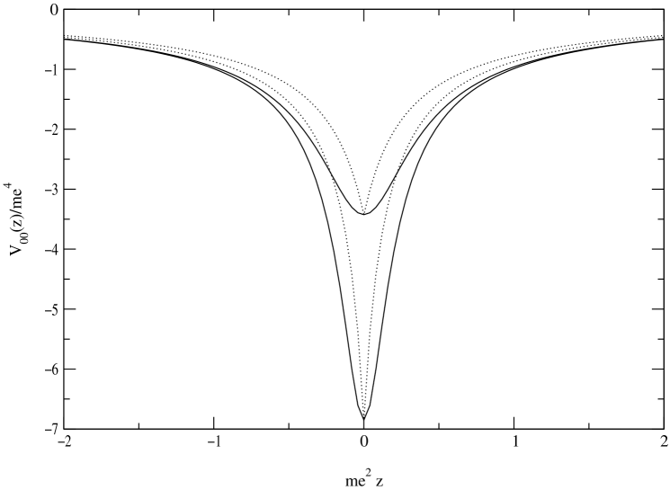
FIG. 1.: Interaction potential of positronium, in units of $me^{4}$, as given by our Eq. (108) (solid lines). We also show for comparison the approximation, Eq. (109) used by Usov and Shabad (dotted lines). In both cases, the deepest curve corresponds to $P_{2}^{0}=2m$, and the other one to $P_{2}^{0}=4m$.

REFERENCES

- [1] L.B. Leinson and V.N. Oraevskii, Sov. J. Nucl. Phys., 42 (1985) 254.
- [2] L.B. Leinson and V.N. Oraevsky, Phys. Lett., 165B (1985) 422.
- [3] H. Herold, H. Ruder, and G. Wunner, Phys. Rev. Lett., 54 (1985) 1452.
- [4] A.E. Shabad and A.V. Usov, Astrophys. Space Sci., 117 (1985) 309.
- [5] D. Koller, M. Malvetti, and H. Pilkuhn, Phys. Let. 132A (1988) 259.
- [6] A.E. Shabad and A.V. Usov, Astrophys. Space Sci., 128 (1986) 377.
- [7] J.F. Avron, I.B. Herbst and B. Simon, Ann. Phys, NY, 114 (1978) 431.
- [8] R. Loudon, Am. J. Phys., 27 (1959) 649.