Th Ages for Metal-Poor Stars

Abstract

With a sample of 22 metal-poor stars, we demonstrate that the heavy element abundance pattern (Z$\geq 56$) is the same as the r-process contributions to the solar nebula. This bolsters the results of previous studies that there is a universal r-process production pattern. We use the abundance of thorium in five metal-poor stars, along with an estimate of the initial Th abundance based on the abundances of stable r-process elements, to measure their ages. We have four field red giants with errors of 4.2 Gyr in their ages and one M92 giant with an error of 5.6 Gyr, based on considering the sources of observational error only. We obtain an average age of 11.4 Gyr, which depends critically on the assumption of an initial production ratio of Th/Eu of 0.496. If the Universe is 15 Gyr old, then the Th/Eu₀ should be 0.590, in agreement with some theoretical models of the r-process.

1. Introduction

One of the fundamental parameters of the Universe is its age. The expansion age of the Universe can be calculated directly from $\Omega_{M}$, $\Omega_{\Lambda}$, and H₀. Since these quantities are not easily measured, a lower limit to the age of the Universe from the ages of the oldest local objects has been an important constraint. As recently as 1996, the most widely-accepted age of the oldest objects was larger than the expansion age of the universe for the then-popular cosmology – a matter-dominated flat universe with $\Lambda=0$ and H${}_{0}\sim 70$ (Bolte & Hogan, 1995). However, results from observations of high-z supernovae suggest a non-zero value for $\Lambda$ and larger expansion ages, 14.2 $\pm$ 1.7 Gyrs (Riess et al. 1998) and 14.9 $\pm^{1.4}_{1.1}$ Gyr (Perlmutter et al. 1999). Furthermore, the ages of the globular clusters, the most stringent local limit, have been revised downward with the lengthening of the Pop II distance scale after Hipparcos satellite parallaxes were measured for nearby metal-poor stars. Carretta et al. (2000) combined results from Hipparcos on the distances to subdwarfs, RRLyrae and Cepheids to re-calibrate the globular cluster distance scale and found an average age for the globular clusters of 12.9 $\pm$ 2.9 Gyrs.

However, it would be valuable to have additional methods, independent of stellar models and the Pop II distant scale, to derive the ages for old stars. It would also be of interest to measure ages for the field halo stars, in particular stars with [Fe/H] $<-2.5$ – more metal-poor than the most chemically deficient globular cluster stars. Butcher (1987) suggested using the abundance of the only long-lived isotope of Th, Th-232, and in particular the Th/Nd ratio, as a method for deriving the ages of field stars. With a half-life of 14.05 Gyrs, Th decays over a cosmologically interesting time. However, Nd is also produced in the s-process, while Th is a pure r-process product, so the Nd production may not track the production of Th through Galactic history (Butcher 1987; Mathews & Schramm 1988). Pagel (1989) suggested using the Th/Eu ratio, as the abundance of Eu is dominated by contributions from the r-process. Francois, Spite, & Spite (1993) measured the Th/Eu ratio in stars with [Fe/H] between $-1$ and $-3$. They found a fairly flat ratio, with perhaps a rise at the lowest metallicities, which they thought implied different chemical evolution histories for these two elements, though a flat ratio would also be expected if there were no age-metallicity relation. Unfortunately, their study was hampered by unknown blending in the Th region, as were the earlier investigations of Butcher (1987) and Morell, Källander, & Butcher (1992).

Sneden et al. (1996) analyzed the metal-poor, but heavy-element-rich, star CS 22982-052. They could measure 16 stable elements from Ba (Z=56) to Os (Z=76), some for the first time in a metal-poor star. They found that abundances for the 16 elements agreed with a scaled solar system r-process pattern (r_ss). Th, on the other hand, was lower than predicted by r_ss. If they assumed that the deviation from the solar r-process pattern was due to the radioactive decay of Th, rather than to a lower initial Th abundance in CS22892-052, they could obtain a lower limit to the age of 15.2 $\pm$3.4 Gyr. This paper included a comprehensive list of transitions in the region of the ThII 4019Å line and the Th abundance was derived via spectrum synthesis. Westin et al. (2000) measured a Th abundance for another metal-poor giant, HD115444, and determined ages for it and CS 22892-052 using theoretical predictions for the production of Th and the stable elements in the r-process. They found an average age of 15.6 $\pm$ 4 Gyr.

Table 1Model Atmosphere Parameters

star	Teff	log $g$	[Fe/H]mod	$\xi$
HD 29574	4350	0.30	-1.70	2.30
HD 63791	4750	1.60	-1.60	1.70
HD 88609	4400	0.40	-2.80	2.40
HD 108577	4900	1.10	-2.20	2.10
HD 115444	4500	0.70	-3.00	2.25
HD 122563	4450	0.50	-2.65	2.30
HD 126587	4675	1.25	-2.90	1.90
HD 128279	5100	2.70	-2.20	1.40
HD 165195	4375	0.30	-2.20	2.50
HD 186478	4525	0.85	-2.40	2.00
HD 216143	4500	0.70	-2.10	2.10
HD 218857	4850	1.80	-2.00	1.50
BD -11 145	4650	0.70	-2.30	2.00
BD -17 6036	4700	1.35	-2.60	1.90
BD -18 5550	4600	0.95	-2.90	1.90
BD +4 2621	4650	1.20	-2.35	1.80
BD +5 3098	4700	1.30	-2.55	1.75
BD +8 2856	4550	0.70	-2.00	2.20
BD +9 3223	5250	1.65	-2.10	2.00
BD +10 2495	4900	1.90	-2.00	1.60
BD +17 3248	5200	1.80	-1.95	1.90
BD +18 2890	4900	2.00	-1.60	1.50
M92 VII-18	4250	0.20	-2.18	2.30

The 4019Å Th line is weak and is blended with several lines of other elements. The errors on the Th-based age estimates are so far dominated by measuring and spectrum synthesis uncertainties for the Th line. It is therefore possible to reduce the error in the mean age derived via this method by making the measurement in additional stars. A second significant source of uncertainty in the Th-based ages is the assumption that the r-process abundance pattern for elements from Ba to Th is “universal” and that the abundance of elements such as Ba, Eu, Nd and Sm can be used to estimate the initial Th abundance in a star. The consistency of heavy-element abundance ratios in studies to date supports a universal r-process pattern. In addition to the spectacular example of CS22892-052, other observations of heavy elements (Z$\geq 56$) in metal-poor stars have in general agreed with the solar-system r-process pattern. Sneden & Parthasarathy (1983) showed that the metal-poor giant HD 122653 has heavy element abundances best explained by a pure r-process contribution that matches r_ss. Gilroy et al. (1988) studied 22 stars with [Fe/H] $<-1.5$ and came to similar conclusions for this larger sample. Sneden et al. (1998) used GHRS spectra to look at three elements in the A=195 peak, Os, Ir and Pt, in three metal-poor stars. Combining these results with ground-based data for other elements, they again confirmed the universality of r_ss in this mass range. In addition to allowing a clean estimate of the initial Th abundance in stars, this result, if substantiated further, is very important for understanding the site of the r-process.

In order to use elements such as Ba and La to estimate the original Th abundance and to test for a universal r-process pattern, we need to make the assumption that the stars we are studying have no s-process contributions. This assumption can be tested since the s-process produces distinct abundance patterns, such as increased Ba and La but not Eu, that would be noticeable in abundance ratios.

To further investigate the nature of r-process abundances and to estimate ages for additional halo stars based on their Th abundances, we have obtained high-resolution, high-signal-to-noise spectra of 23 metal-poor stars. In five of these stars, the abundance of neutron-capture elements is high enough that Th is detectable. We estimate ages for these stars to provide a lower limit to the age of the Universe independent of the globular clusters. We use 22 field stars to test the validity of the assumption of universal r-process pattern.

2. Observations and Data Reductions

The stars observed are metal-poor ([Fe/H] $<$ $-1.7$) field giants from the list of Bond (1980) along with one giant in the globular cluster M92. The data were obtained with two instruments. “HIRES” is the echelle spectrograph at the Keck I telescope (Vogt et al., 1994). These data cover 3200-4700 Å, with R$\sim$ 45,000 and a signal-to-noise greater than 200 at 4000Å for almost all stars. HIRES data of 12 stars were obtained in May and June 1997. The second instrument was the Hamilton spectrograph on the Shane 3-meter telescope at Lick Observatory (Vogt, 1987). The Hamilton spectra cover the range 3800-7900 Å, with a S/N of $\sim$ 100 at 6000 Å. We obtained Hamilton spectra for 10 of the HIRES stars, as well as 11 additional Bond giants. The Hamilton spectrograph data were taken to obtain additional lines in the red, particularly Fe and Ti lines, to help refine the model atmosphere parameters. We also wanted to survey additional Bond giants to add to the sample of stars with many heavy elements measured, and to find more stars with high [r-process/Fe] as possible candidates to measure Th. The spectra were flat-field corrected, bias-corrected, extracted and wavelength-calibrated using IRAF (Tody 1993). The equivalent widths (EWs) of many light and heavy elements were measured using SPECTRE (Sneden, private communication). Abundance analysis was done using MOOG (Sneden 1973). The log of observations can be found in Johnson (2001) (Paper II).

Figure 1.— Synthesis of the Th region in stars with low [heavy-element/Fe] ratios. Only upper limits on the Th abundance could be determined. The good fit with the observations indicates that our list of lines that blend with the Th line is reasonably complete and accurate. Our synthesis predicts more absorption at 4018.836 Å than is seen because our NdII abundances in heavy-element-poor stars are too high.

Figure 2.— Synthesis of the Th region in HD 115444 and HD 186478. The left panel shows the overall synthesis with the best-fit Th abundance, as well as the individual contributions of the major contaminants Fe and ¹³CH. The right panel shows the best synthesis and the change in the fit if the Th abundance is changed by $\pm$ 0.10 dex.

Figure 2.— Synthesis of the Th region for BD +8 2548 and M92 VII-18. See figure caption for Figure 2a.

Figure 2.— Synthesis of the Th region for HD 108577. See figure caption for Figure 2a. The fit to the data would be improved if the FeI abundance was $\sim$ 0.5 dex lower than the value adopted from EW analysis. However, the derived Th abundance would not change.

3. Model Atmospheres

We used the updated model atmospheres of Kurucz (http://cfaku5.harvard.edu/). Our choices of model atmosphere parameters are discussed fully in Paper II, and we summarize the results in Table 1. In brief, we set the microturbent velocity ($\xi$) by requiring there be no correlation between the derived abundance from the CaI, CrI, FeI and TiII lines and their reduced EWs (RW=EW/$\lambda$). While many of the other elements showed no trend in abundance as a function of logRW at our adopted $\xi$, some elements showed trends that changes of up to $\sim\pm 0.3$ km/s in $\xi$ eliminated. We have chosen $\pm 0.3$ km/s as our error in $\xi$. T_eff was changed until there was no trend in the abundance versus excitation potential plot of the FeI lines. We estimate, based on the range of T_eff that produce acceptable fits, that our errors are $\pm 100$K. Next, we determined log $g$ by matching the FeI and FeII abundances. We have only $\sim$ 15 FeII lines and the gf values for these are generally of lower quality than those for FeI lines. Our FeII abundances therefore have a relatively large standard deviation of the mean $\sim$ 0.05. Also our gravities depend on our choice of temperature and $\xi$, so our errors in log $g$ are $\pm$ 0.3 dex. Changing the metallicity of our atmosphere by 0.2 dex only changed the abundances by $\pm$ 0.01 dex, and therefore that has been ignored as a source of error.

4. Abundances

4.1. Heavy Elements

We attempted to determine the abundances for many heavy elements from Ba (Z=56) to Os (Z=76) in the stars we observed to see if r_ss was repeated in these stars. The stars in our sample were more metal-rich than CS22892-052 as well as less heavy-element rich. Therefore, blending and detection affected some of the lines that Sneden et al. (1996) could use in their study of CS22892-052. We included only those lines which were not affected by blending at the line center, with the exception of Th (see below). Excluding blended lines meant we were not able to measure every element in every star. In particular, for Ho, Hf, and Os, we were able to obtain upper limits only, which are still useful in ruling out large ($\sim$ 0.5 dex) deviations in the r-process pattern. Unfortunately, the line we could use to set limits on the Os (4261.85 Å) gave a lower abundance by $\sim$0.50 dex than other lines used by Sneden et al. (1996). for CS 22892-052. Line parameters and EWs are listed in Paper II. Hyperfine splitting was taken into account for Ba, La, Eu, and Ho. Based on the abundance pattern seen in the other elements, we adopted the Ba abundances derived using the solar system r-process isotopic composition. Choosing the total solar system isotopic composition increased the Ba abundances by $\sim 0.02-0.05$. Whenever possible, we used analysis of EWs of lines to derive abundances of unblended lines. Spectral synthesis was used in crowded regions. Our linelists are from Sneden et al. (1996). Table 2 summarizes our heavy element abundances. For solar values we have used the photospheric abundances for Anders and Grevesse (1989), except for those elements with uncertain photospheric abundances where meteoritic values were used. We also adopted log $\epsilon$=7.52 as the solar iron abundance.

4.2. Th Abundance

The only Th line strong enough to measure in our spectra (4019.12 Å) is unfortunately blended with several lines from other elements. We made an initial line list based on the atomic data of Morell et al. (1992), Sneden et al. (1996) and Kurucz CD ROM 23. We then synthesized the solar spectrum using these lists and adjusted the gf values of lines to match the solar spectrum. For crucial lines, we searched the literature for laboratory values. For the FeI line, we adopted a log gf of $-2.68$ from May (1974) and a wavelength of 4019.043 Å from Learner et al. (1990). The Th line also has a wavelength from Learner et al. and a laboratory log gf from Simonsen et al. (1990). The hyperfine $A$ and $B$ constants for the CoI lines at 4019.13 Å and 4019.29 Å are given in Pickering & Semeniuk (1995). Norris, Ryan & Beers (1997) pointed out the important contribution of ¹³CH lines from the $B\Sigma^{-}-X^{2}\Pi$ 0,0 band and suggested that Kurucz’ estimated wavelengths be adjusted by 0.15-0.25 Å. We have a spectrum of the extremely carbon-rich star, CS 22957-057, that drew Norris et al.’s attention to the ¹³CH contamination. This is a lower S/N ($\sim$ 50) spectrum taken with HIRES during the June run. Our spectrum confirms the wavelengths for the ¹³CH lines found by Norris et al.. The gf values for the ¹³CH lines have been taken from Kurucz’s web site. Finally, the CeII line can be important in stars with supersolar [Ce/Fe] ratios. Sneden et al. (1996) found it necessary to include this line in order to account of the absorption profile in CS22892-052. They increased the log gf value by 0.3 dex over the value from Kurucz’ CD-ROM 23. It made a difference of 0.05 dex in the derived Th abundance in CS 22892-052. Here, with better resolution and smaller CeII abundances, that increase in the Ce II gf affects the Th abundance at most $\pm$ 0.02. Table 3 has the linelist we used, which contains lines up to 1/1000 the strength of the Th line in red giants.

Table 3Linelist near ThII at 4019 Å

$\lambda$ (Å)	Element	E.P. (eV )	log gf
4018.100	Mn I	2.11	-0.309
4018.266	Fe I	3.27	-1.360
4018.368	Zr II	0.96	-0.994
4018.506	Fe I	4.21	-1.597
4018.836	Nd II	0.06	-0.880
4018.986	U II	0.04	-1.391
4019.000	13CH	0.46	-1.163
4019.043	Fe I	2.61	-2.680
4019.057	Ce II	1.01	0.093
4019.067	Ni I	1.94	-3.174
4019.110	Co I	2.28	-3.287
4019.118	Co I	2.28	-3.173
4019.120	Co I	2.28	-3.876
4019.125	Co I	2.28	-3.298
4019.125	Co I	2.28	-3.492
4019.130	Th II	0.00	-0.270
4019.134	Co I	2.28	-3.287
4019.135	Co I	2.28	-3.474
4019.137	V I	1.80	-1.300
4019.138	Co I	2.28	-3.173
4019.140	Co I	2.28	-3.298
4019.170	13CH	0.46	-1.137
4019.272	Co I	0.58	-3.480
4019.281	Co I	0.58	-3.470
4019.294	Co I	0.58	-3.220
4019.296	Co I	0.58	-3.330
4019.322	Co I	0.58	-4.090
4019.332	Co I	0.58	-4.040
4019.632	Pb I	2.66	-0.220
4019.726	Gd I	0.07	-1.046
4019.810	Nd II	0.63	-0.770
4019.829	Sm II	0.28	-1.695
4019.880	Fe I	2.60	-5.000
4019.897	Ce II	1.01	-0.368
4019.976	Sm II	0.19	-1.419
4020.029	12CH	0.46	-1.163
4020.051	Nd II	1.27	-0.290
4020.193	12CH	0.46	-1.137
4020.251	Ni I	3.70	-0.936
4020.390	Sc I	0.00	0.039
4020.482	Fe I	3.64	-1.900

For every synthesis in the Th region, the Fe, Ni, Nd, and Co abundances were the abundances previously deduced from the EW analysis. The ¹²CH lines from the same transition as the contaminating ¹³CH lines are at 4020 Å. Therefore, the carbon abundance of a star was adjusted to match the 4020 Å feature. The ¹²CH/¹³CH ratio was determined using lines between 4200-4370Å and is listed in Table 4 for stars with Th abundances. Because the ¹³CH lines in our sample were weak, these ratios have errors of $\pm 2$. Ce could only be measured in the neutron-capture-rich stars. For the other stars, our Ce values were estimated using the Ba abundance and the Ce/Ba ratio found in the neutron-capture-rich stars, an assumption which is justified by the results in §5.1.

Table 4¹²CH/¹³CH used for Thorium Synthesis

Star	12CH/13CH
HD 186478	6
HD 115444	6
HD 108577	4
BD -18 5550	32
HD 122563	6
BD +4 2621	8
HD 128279	32
M92 VII-18	4
BD +8 2548	6

We tested the validity of the linelist of contaminants on four stars with high S/N, but low [heavy-element/Fe] values (Figure 1). For these stars we expect little contribution of Th, Nd or Ce to the region. In each case, we set the Th to be as large as possible. These upper limits are included in Table 2. The agreement between synthesized and observed spectra in Figure 1 is encouraging, especially since the amount of absorption due to Fe and ¹³CH varies from star to star. For the high [heavy-element/Fe] stars, Figure 2 shows our best synthesis with the individual contributions of the strongest lines in one panel and the effect of changing the Th abundance in the second panel. The Th abundance results are included in Table 2.

4.3. Error Analysis

A complete discussion of the error analysis can be found in Paper II. We consider two sources of error for each element: line-by-line scatter caused by errors in gf values and EWs and systematic offsets caused by incorrect model atmospheres. For elements with several measurable lines, we estimate the random errors with the standard deviation of the mean of the abundance. For stars with only one or a few lines of a particular element, we established a minimum standard deviation by looking at the standard deviation for that element in stars with many lines or by looking at errors in the EWs or spectral synthesis. Table 2 lists the standard deviation of the sample ($\sigma$) for each element, as well as the number of lines used to determine the abundance. Also given is the error in [element/H] ($\sigma_{tot}$), where the errors associated with the model atmospheres are taken into account.

Since only the relative abundances, rather than absolute [element/H], are important for this method of determining ages, we performed new numerical experiments to calculate the errors in the relative abundances of the heavy elements as the atmospheric parameters are changed. For the elements between Z of 56 and 70 as well as Th, we determined the change in the abundance if we changed the temperature by 100K, log g by 0.3 dex, or $\xi$ by 0.3 km/s. The abundances of rare earth elements and Th change in similar directions when the model atmospheres change, leaving only a small relative difference. The exception is Ba and Yb when $\xi$ is changed, because these elements are usually only represented by much stronger lines than the rest of the heavy elements. In addition, in many cases, the abundances change the same way with an increase in T_eff and an increase in log $g$. Since these quantities are anti-correlated along the red giant branch, the net effect of changing the model atmosphere parameters is further decreased. The overall error in abundances of the rare earths relative to each other from the choice of model atmosphere parameters is negligible compared with the line-by-line scatter. For example, the error in [Nd/Ce] from the model atmospheres is $\sim$ 0.01 and for [Sm/Eu] it is $\sim$ 0.05, smaller than the line-by-line uncertainties of $\sim$ 0.05-0.2 dex. With these results in mind, we will use as errors the standard error of the mean when focusing on these elements.

Figure 3.— Abundances for HD 115444(open squares), HD 186478(crosses), HD 108577(triangles) and BD +8 2548(filled circles). They have been scaled to match the Arlandini et al. (1999) solar system r-process curve using the mean difference between the Sm, Eu, La, Ba and Ce abundances. We also show the Käppeler et al. (1989) r-process curve to illustrate the errors present in deriving solar-system r-process contributions. The differences between the two curves arise because of improved nuclear data and different physical conditions used during the s-process. These s-process predictions are then subtracted from the total solar-system abundances to produce the curves shown here.

The Th abundance reacts to changes in the model atmosphere parameters in a very similar manner to the stable neutron-capture elements. However, because the Th line is blended, it is possible that the relative importance of the contaminants could change because the [Th/Fe] and [Th/C] ratios do depend on the model atmospheres. ¹²CH/¹³CH was determined using weak ¹³CH lines and as a result the error in the ¹³CH contribution is dominated by the error in the ¹²CH/¹³CH ratio, rather than the choice of model atmosphere parameters. As mentioned earlier, the accurate knowledge of [C/H] is not important. The Fe line does not overlap with the Th line as much as the ¹³CH line and can be monitored independently by looking at the left wing. As a result, error in the [Th/neutron-capture] ratio from the model atomsphere parameters is surprising small $\sim$ 0.03 dex. Our total error budget for the Th abundance includes 0.05 dex for continuum placement and errors in the contributions of the contaminants and 0.05 dex due to uncertainties in the ¹²CH/¹³CH ratio.

We have one final note on errors. Our NdII values appear to be biased $\sim$ 0.2 dex high in Nd-poor stars. In Nd-rich stars, the two strongest lines, at 4061.09 Å and 4109.46 Å, the only ones that we can measure in the Nd-weak stars, systematically give higher abundances than the other lines. We believe that the large abundances given by the two strongest lines can be traced to errors in gf values. The Nd lines in general show large scatter, larger than can be explained by errors in EW or model atmosphere parameters. Also, Thevenin (1989), in his compliation of solar gf values, found log gf values for these two lines that were large by 0.2 dex. We have chosen not to correct the Nd-poor stars’ values, but caution the reader on the accuracy of NdII measurements based on fewer than 3 lines. This situation will hopefully soon be eliminated with the measurement of new NdII gf values. This strong line gf problem does not appear to affect any of the other elements.

5. Results

5.1. The heavy-element abundance pattern

The exciting possibility of using Th abundances to estimate ages of individual stars depends on the reliability of deriving the initial Th abundance for a star based on the abundance of stable elements. The investigations to date suggest a single (or at least a dominant) “universal” r-process abundance pattern, presumably reflecting the physical conditions in the r-process site (see earlier discussion). Although we can only determine a Th abundance in some of the stars, we can use all the field stars to further investigate the universality of r-process abundance ratios. (We did not use M92 VII-18 for this part of the discussion because of the lower S/N of its HIRES spectrum and the lack of Hamilton data). For a qualitative idea of how well our abundances matched r_ss, we plotted the abundances from the four field stars with thorium measurements and two predictions for the r-process contributions to the solar system abundances (Figure 3). There is good agreement between our data and r_ss, and no obvious s-process contribution, even for the more metal-rich ([Fe/H]$\sim-2.1$)

5.1.1 The s-process contribution

The onset of substantial s-process contributions to the heavy elements is the subject of much debate. CS22892-052 shows no sign of s-process contributions for Z$\geq$56 (Sneden 1996). Neither do HD 115444 ([Fe/H]$\sim-3.0$) or HD 122563 ([Fe/H]$\sim-2.7$) (Westin et al. 2000). McWilliam (1998) measured [Ba/Eu] for 14 stars with [Fe/H]$<-2.0$; With the exception of two CH-stars and one star with [Fe/H]$=-2.07$, this sample showed r-process [Ba/Eu] ratios. He proposes that only stars more metal-rich than [Fe/H]$\sim-2.0$ show s-process contributions. Cowan et al. (1996) found that an addition of 20% of the total solar system s-process abundances to r_ss gave a better fit to the abundances of HD126238 ([Fe/H]$\sim-1.7$) Recent models of Galactic chemical evolution (Raiteri et al. 1999; Travaglio et al. 1999) predict that s-process contributions to the Galactic Ba abundance appear at [Fe/H]$\sim-1.7$.

Other studies have found substantial contributions from the s-process in stars with [Fe/H]$<-2.0$. Magain (1995) argued that the profile and width of the BaII line at 4554 Å in the subgiant HD 140283 ([Fe/H]$\sim-2.6$) agreed with a dominant contribution from Ba isotopes produced only in the s-process. These even isotopes are not affected by hyperfine splitting, leading to a more pronounced line core. Mashonkina, Gehren & Bikmaev (1999) studied the barium abundances in cool metal-poor dwarfs. They found that they could not match the equivalent widths of the 4554 Å line with the barium abundances derived from weaker lines unless they adopted a solar ratio of s- to r-process Ba contributions. Otherwise the strongest Ba line demands a Ba abundance that is 0.2-0.3 dex lower than the other lines. Unfortunately, the same effects could be mimicked by changes in microturbulent velocity or changes in temperature structure in the atmosphere, including the addition of the chromosphere. We find that using an r-process isotope distribution decreases the spread in Ba abundances derived from different lines in our sample of giants. A complicating factor in using the Ba isotopes as s-process vs. r-process discriminators is the unknown contributions of the even Ba isotopes to the r-process abundances. ¹³⁴Ba and ¹³⁶Ba are blocked from contributions to the r-process by stable nuclei; ¹³⁸Ba is not. Käppeler et al. (1989) found that all ¹³⁸Ba can be made in the s-process, leaving no need for an r-process contribution, while Arlandini et al. (1999) found that over half of the Ba made in the r-process comes from ¹³⁸Ba. Mashonkina et al. (1999) excluded ¹³⁸Ba from their r-process isotope mix. As discussed in more detail below, if we look at weaker lines of other elements which are more immune to changes in $\xi$ and the temperature structure in the upper layers of the atmosphere, we confirm that the maximum s-process contribution to even the most metal-rich star in our sample is $\sim$ 10%.

Burris et al. (2000) argued on the basis of [Ba/Eu] ratios for 43 giants that contributions from the s-process began at [Fe/H]=$-2.9$ Comparing log $\epsilon$ for the 17 stars we have in common, we find a 0.1 dex larger average offset between their log $\epsilon$(Ba) and ours than we do for the log $\epsilon$(Eu). While an offset is expected because of the different model atmospheres, a different offset between two rare earth elements is a cause for concern. As indicated by the previous paragraph, analysis of Ba is difficult problem, especially the analysis of the strongest line at 4554Å, which is the only line available for about a third of the stars in the Burris et al. sample. Their Ba abundances were on average 0.21 dex larger than McWilliam (1998) for stars they had in common.

Figure 4.— (a) [Ba/Eu] vs. [Fe/H] and (b) [La/Eu] vs. [Fe/H] for our sample and the Burris et al. (2000) sample. There is no trend for increasing [La/Eu] as [Fe/H] increases, as would be predicted by the [Ba/Eu] results. We believe that both sets of Ba abundances become increasingly unreliable as [Fe/H] increases, because of the strong dependence of Ba on $\xi$. Our [La/Eu] values are consistent with only a solar system r-process contribution. The offset between the two data sets in [La/Eu] is most likely a result of somewhat different linelists combined with imperfect gf values. Since we have 17 stars in common, the offset is not due to markedly different samples of stars. The solar system r-process ratios are from Arlandini et al. (1999). The poor agreement between the solar system r-process and the lower limit for our [Ba/Eu] could be due in part to uncertainties in the solar system predictions (see Figure 3).

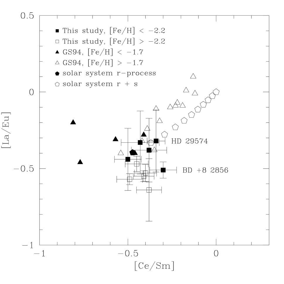
Figure 5.— Two s-process sensitive ratios, [La/Eu] and [Ce/Sm]. The filled pentagon marks the prediction of Arlandini et al. (1999) for pure r-process abundances. The open pentagons mark the addition of s-process material in increments of 10% of the total solar s-process abundance. For our data, the more metal-rich stars have a higher [La/Eu] due to biased Eu values as discussed in the text, but their [Ce/Sm] values are in agreement with no s-process contribution, with the exception of HD29574. While the Gratton & Sneden (1994) stars with [Fe/H]$>-1.7$ follow the path of increasing s-process contributions in spirit if not in exact numbers, the stars with [Fe/H]$<-1.7$ show no such inclination.

They attributed this to their smaller microturbulent velocities. We have plotted in Figure 4 the [Ba/Eu] and [La/Eu] ratios from both Burris et al. and this study. 75% of the solar abundance of La is provided by the s-process, so this ratio is as sensitive to s-process contributions as [Ba/Eu]. Figure 4 shows that for both our sample and the Burris et al. sample, there is no trend toward increasing [La/Eu] at higher metallicities. To be consistent with their [Ba/Eu] results, [La/Eu] would need to be $\sim$0 for the most metal-rich part of their sample. We feel the La abundances in both samples are the more robust, and therefore believe that the [La/Eu] ratios show the true s-process situation. Finally, although the scatter in our [La/Eu] presented in Figure 4 is consistent with being due to observational errors only, there could be stars with some small fraction of s-process among our sample.

We have carried out a simple test with our data using two s-process sensitive ratios to check for s-process contributions. Figure 5 shows [Ce/Sm] vs. [La/Eu] for the nine stars in our sample that have measurements of these four elements. These fall into two groups: the relatively neutron-capture rich stars that were used for Th measurements and the more metal-rich ([Fe/H]$>-2.2$) stars that have measurable Ce and Sm lines. We see that for one star (HD 29574, [Fe/H]=$-1.7$) an s-process contribution of 10% could be allowed, while the rest of those with higher [La/Eu] ratios have [Ce/Sm] ratios that agree with the more metal-poor stars. The offset between the neutron-capture rich and the metal-rich groups in [La/Eu] is because the metal-richer stars have their Eu abundances based solely on the 4129Å line. The metal-richer stars were preferentially observed only with the Hamilton, and the 4129Å was all that was available at reasonable signal-to-noise in the Hamilton data. Figure 7 shows that this biases the Eu abundances low. The exception is BD+8 2548, which is both metal-rich and neutron-capture-rich, and has the lowest [La/Eu] of the metal-rich group. We have also plotted in Figure 5 the data from Gratton & Sneden (1994) who suggested a contribution from the s-process beginning at [Fe/H]$<-2.0$ as a possible explanation for their heavy element abundances. We see that below [Fe/H] $<-1.7$ their data do not show the trend expected with an s-process contribution, while the more metal-rich stars ($-1.7\leq\rm{[Fe/H]}\leq-0.15$) show the rising [La/Eu] and [Ce/Sm] ratios that is the signature of increasing s-process contributions. There is large scatter and offsets from our data present in their abundances, especially in the metal-poor stars, which we attribute to different, and more uncertain, gf values used in the Gratton & Sneden (1994) study. In summary, we find no convincing evidence for large s-process contributions, either in our sample, the Burris et al. sample or in the metal-poor Gratton & Sneden sample. For the rest of our analysis, we will assume that the heavy-element abundances in our sample of stars represent contributions from the r-process only.

Figure 6.— $\Delta(\rm log\epsilon)$ between each star’s abundance and the mean abundance for all stars. Here we have used for the mean calculation only measurements based on 3 or more lines, except for Tm, Tb and Yb, which are usually represented, even in the most heavy-element-rich star, by one line. These measurements are plotted with the big squares. The error bars represent an average 1-$\sigma$ error bar of the restricted sample for an individual data point. The error bars are large enough to explain the scatter. We also plotted the difference between the mean value and measurements based on fewer than three lines as small squares. The abundances of Nd and Eu, in particular, show the advantage of having multiple measurements.

5.1.2 The r-process pattern

Next, we wanted to determine quantitatively if all of the metal-poor stars we observed showed a universal r-process pattern in their heavy element abundances. For each of the stars observed, we used r_ss as a template to put all of the heavy-element abundances in the stars on a common scale. We used the mean difference between the Sm, Eu, La, Ba and Ce abundances in the star and the solar abundances attributed by Arlandini et al. (1999) to the r-process to scale each star up, regardless of its [Fe/H] and [heavy-element/Fe] values. We then restricted the sample to abundances that were determined using three or more lines, with the exception of Tb, Tm and Yb abundances, which, even in the most favorable cases, were always determined with 1 or 2 lines. We found the mean value for each element among this scaled, restricted sample. The deviation of each star from these mean values is recorded in Figure 6. The large symbols indicate measurements which contributed to the mean, while the small symbols show all the other deviations. The larger scatter and bias in the Nd and Eu measurements among the small symbols show the inherent problems of relying on one or two lines.

Figure 7.— A comparison between the abundances in the metal-poor stars and the r-process contributions to the solar system abundances. The open circles (with 1-$\sigma$ error bars) represent the average deviation from the well-measured abundances in the metal-poor stars from the scaled r_ss. There are no differences observed at the 2-$\sigma$ level.

The first question to ask about the distribution in Figure 6 is whether the observational errors in the individual points are large enough to account for the star-to-star scatter for each of the elements. We consider only the random errors and the errors from the overall scaling. We calculated the latter in a simplistic manner by finding the average standard deviation of the mean of our five determinations of the shift for each star. This was added in quadrature to the average random error of the restricted sample in the abundance determination to produce the error bars in Figure 6. In general the error bars are large enough to account for the observed dispersion. The exception might be Ba, but that is the one element for which our assumption that we could exclude model atmosphere errors is the most unreliable, since Ba has a large dependence on $\xi$. Therefore, we argue that the scatter can be attributed entirely to the observational errors.

We also calculated the difference between each star’s abundance and r_ss. In order to have a true differential comparison between the abundances in our sample and in the Sun, we used the total solar abundance derived from the lines that we could measure in the metal-poor stars, rather than the values of Anders & Grevesse (1989). The r-process fractions were adopted from Arlandini et al. (1999).

Figure 8.— Ages from Th abundances. We have plotted the Case 3 and Case 4 results. In most cases the two different scalings agree very well; the exception is HD 115444 which reflects the reality of our 0.05 dex observational errors in the rare earths. Also plotted is the average age derived by Westin et al. (2000) from HD 115444 and CS 22892-052.

We plot the mean difference between the restricted sample and r_ss, as well as the s.d.m, in Figure 7 to determine whether the pattern observed in metal-poor stars is the same as r_ss. For the errors in the solar values, we include the errors in the solar-system r-process fraction and in the total solar abundances. The fraction of the abundance of an element in the solar system contributed by the r-process is determined by subtracting the amount attributed to the s-process from the total abundance. While the conditions where the s-process occurs and the relevant nuclear cross-sections and decay-rates are better known than for the r-process, errors of 5% in the predicted s-process abundances are not uncommon (e.g. Käppeler, Beer, & Wisshak 1989). For the elements that are contributed to the solar nebula primarily by the s-process, such as Ba and La, this can lead to substantial errors in r_ss. In Figure 7, we use the errors in the solar-system r-process determinations from Arlandini et al.(1999), which are based on considering uncertainties in cross-sections and in the physical conditions where the s-process occurs. To estimate the uncertainty in the total solar system abundance, we use the difference between the photospheric and meteoritic abundances from Anders & Grevesse (1989), except for those differences listed as uncertain, in which case we use 0.04 dex. Some part of these difference may be attributed to gf errors, which we have eliminated by using the differential comparison above. However, substantial errors also exist because of blending, the choice of the solar model atmosphere, damping constants and continuum placement, and we hope to provide some idea of those by using the difference between the photospheric and the meteoritic abundances. Figure 7 shows no deviations from r_ss at the 2-$\sigma$ level. In summary, our results are consistent with a single r-process pattern being present in metal-poor stars and in the Sun from elements with Z$\geq$56.

5.2. Ages

Table 5Ages from Th Abundances

Star	log$\epsilon$(Th)	log$\epsilon$(Th0)	log$\epsilon$(Th0)	log$\epsilon$(Th0)	log$\epsilon$(Th0)	Age(Gyr)	Age(Gyr)	Age(Gyr)	Age(Gyr)
		(1)	(2)	(3)	(4)	(1)	(2)	(3)	(4)
HD 186478	$-2.26$	$-1.90$	$-1.90$	$-1.87$	-1.87	$>16.8$	$>16.8$	18.3	18.3
HD 115444	$-2.36$	$-2.27$	$-2.15$	$-2.23$	$-2.12$	$>4.2$	$>9.8$	6.1	11.2
HD 108577	$-1.99$	$-1.79$	$-1.81$	$-1.76$	$-1.78$	$>9.3$	$>8.4$	10.6	9.8
BD +8 2548	$-1.66$	$-1.46$	$-1.50$	$-1.43$	$-1.47$	$>9.3$	$>7.5$	$10.8$	$8.9$
M92 VII-18	$-1.95$	$-1.81$	$-1.79$	$-1.78$	$-1.76$	$>6.5$	$>7.5$	$7.9$	$8.8$

To find the age of a star from its present Th abundance, we need to estimate the initial Th abundance. (We are assuming that the metal enrichment for these metal-poor stars happened over a short period of time, so we do not need to model Galactic chemical history). Given the results in the previous section justifying the use of the scaling factor for stable r-process elements for predicting initial Th abundances we still require an estimate of the original (Th/stable-r-process) ratio. There are two possibilities for estimating this ratio. The empirical approach is to take the present abundance of Th in the Sun, correct it for 5 Gyrs of known decay and use that abundance (log$\epsilon(\rm{Th})_{0,\odot}=0.17$) as a lower limit to the (Th/stable) production in the r-process. In reality, of course, the Sun is made up of gas that has been polluted many times with Th and stable r-process elements over its history. The Th has been decaying over that period, resulting in a smaller (Th/stable) than if it had all been created 5 Gyrs ago. In order to turn a lower limit for the age into an actual value, the Th-production history in the solar neighborhood must be taken into account (e.g. Cowan et al. 1999). Also, different stable elements can give different predictions for the initial Th abundance. An alternative is to use theoretical predictions of (Th/stable). The main disadvantage there is that the r-process nuclei are descendants of isotopes near the neutron-drip line, which have very few laboratory measurements of their properties. Goriely & Clerbaux (1999) found that the predicted Th/Eu₀ ratios vary from 0.25 to 1.55, depending on which theoretical model for nuclear properties was used and which solar r-process abundances near A$=$200 were used as constraints. If the abundance of ²⁰⁹Bi was used, the predicted initial Th/Eu ratio was up to 10 times lower than if the abundance of ²⁰⁶Pb was used. Cowan et al. (1999) regarded the solar r-process abundances as uncertain, and chose instead to focus on those models which gave reasonable agreement with the solar-system r-process abundances over a large range of A, including A$\sim$200. They found that the best fits were given by three models that gave values of Th/Eu₀ of 0.496, 0.546 and 0.48. The situation will be substantially improved as better predictions for the s-process contribution to the Pb and Bi abundances become available (e.g. Travaglio et al. 2000). We calculate the ages of five of the stars in our sample using both the empirical and the theoretical methods, as well as deriving our initial Th abundances based on only the Eu abundances versus all of our well-measured heavy abundances (Table 5). Eu is produced almost exclusively in the r-process (only 5% is due to the s-process), so our derived ages are immune to any possible s-process contributions.

Case 1 refers to the initial Th estimate obtained by scaling the solar Th abundance at the time of the solar system formation by the average offset between r_ss and Ba, Ce, Nd, Sm and Eu in the metal-poor stars. Case 2 scales the solar abundance by the offset between r_ss and Eu. Case 3 has the same scaling as Case 1, but the initial Th abundance is taken from theoretical predictions (Th/Eu₀=0.496), while Case 4 takes the Case 3 initial Th and the Case 2 scaling. Figure 8 shows the Case 3 and Case 4 scalings. The error in the age depends on the error in the present Th abundance ($N_{Th}$) and $N_{Th,0}$.

$$\delta t=\tau\sqrt{\delta(lnN_{Th,0})^{2}+\delta(lnN_{Th})^{2}}$$ (1)

where $\tau$ is the mean life of ²³²Th

$$\tau=20.3Gyr$$ (2)

Errors in $N_{Th,0}$ are caused by observational errors in the measurement of stable r-process element abundances and theoretical errors in the Th/Eu ratio predicted by r-process models. Right now we will consider only the random observational errors of 0.05 dex in log$\epsilon$(stable-r) and the 0.03 dex previously discussed for differential changes in Th and the rare earths when the atmosphere is changed ($\delta$ log $\epsilon$(Th)₀ =0.06). Errors in log$\epsilon$(Th) were discussed above and are 0.07 dex in log$(\epsilon_{Th})$, except for M92 which has larger observational errors of 0.11 dex. Using those errors, we get $\delta t=\pm 4.2$ Gyrs for the field giants and $\delta t=\pm 5.6$ Gyrs for M92. We note that our age for HD 115444 using the Ba, Ce, Nd, Sm and Eu scaling is substantially younger than when using only Eu scaling. Figure 3 shows that is due to the low value of Ba we measured in this star, which produces a lower overall scaling than that suggested by Eu alone. We can find no obvious mistakes in our Ba abundance, nor is the dispersion in the abundances derived from the Ba lines particularly large, but then the offset is only about $-$0.1 dex.

The absolute answer also depends on the log gf value of the Th line at 4019.12 Å. Lawler et al. (1990) gave its error as $\pm 0.04$ dex, which leads to an systematic uncertainty in the age of $\pm$ 2 Gyr. Finally, the chosen Th/Eu₀ is another source of systematic error. We summarize our errors, both observational and theoretical, in Table 6 and show their effect on our age determinations.

Table 6Summary of Errors

Cause of Errors	Error	Error in Gyr
Errors for present $\epsilon$(Th)
12CH/13CH ratio	0.05 dex	2.3
Continuum placement and other blends	0.05 dex	2.3
Total for log$\epsilon$(Th)	0.07 dex	3.0
Errors for $\epsilon$(Th)0
Changes in Model Atmospheres	0.03 dex	1.4
Scatter of log $\epsilon_{r,stable}$	0.05 dex	2.3
Total for log$\epsilon$(Th)0	0.06	2.8
Systematic errors
Uncertainties in log gf	0.04 dex	2.0
Uncertainties in (Th/Eu)0
Goriely & Clerbaux (1999)	$\pm{1.05\atop 0.28}$	$\pm{23.0\atop 14.2}$
Cowan et al. (1999)	$\pm{0.05\atop 0.02}$	$\pm{2.1\atop 0.5}$

6. Discussion

Table 7Derived Th/Eu₀

Star	Age
	12 Gyr
	(Th/Eu)0
HD 186478	0.36
HD 115444	0.52
HD 108577	0.53
BD +8 2548	0.57
M92 VII-18	0.57

The average age for the stars from Case 4 in Table 5 is 11.4 Gyr. We chose Case 4 because Case 1 and Case 2 provide only upper limits, while Case 3 is affected by the low Ba value of HD 115444 (see above). Using the Eu scaling also provides a direct comparsion with theoretical predictions of Th/Eu₀. If we vary the Th/Eu₀ from 0.48 to 0.546, our average age ranges from 10.9 to 13.5 Gyr. All of these values are well within the expansion ages derived by Perlmuter et al. (1999) and Riess et al. (1998). We note that in deriving the Th abundances with spectral synthesis, if the line list for the Th region is incomplete, we will systematically overestimate the Th abundance and underestimate the age of the stars.

For HD115444, Westin et al. (2000) found an age of 15.0 Gyr for (Th/Eu)₀=0.496, compared with 11.4 Gyr for this paper. A comparison of the sytheses of the Th region suggests the main difference is the CH abundance. Their synthesis shows more absorption at 4020 Å than the observed spectrum, which translates into more ¹³CH absorption near the Th line and a smaller Th abundance. However, a more detailed assessment is not possible because they do not give the CH and Fe abundances that they used to obtained their fit. We note that the same ¹³CH/¹²CH ratio was used in both analyses.

Our mean age is based on the assumption of a universal r-process pattern. Previous studies have shown that when the lighter neutron-capture elements are considered as well, there is not a consistent pattern in different stars. For example, McWilliam (1998) found variations as large as 2 dex in the [Sr/Ba] ratio in his sample of metal-poor ([Fe/H]$<-2.5$ giants. Westin et al. (2000) did a differential comparison of HD 115444 and HD 122563, and also concluded the differences were larger than could be explained by their observational errors. Both of these studies, however, showed a single pattern from Ba to the higher Z elements. Our analysis gives a similar result: regardless of the [heavy-element/Fe] value, the abundance pattern from Z=56 to Z=70 cannot be distinguished from r_ss. Goriely & Arnauld (1997) argued that the agreement between the r_ss and metal-poor stars is more a reflection of the underlying nuclear properties of the elements rather than similarity in conditions at the r-process site. Therefore, agreement with a scaled r_ss over a limited range does not imply at similar scaling at Z=90. The observational results that the third r-process peak elements Os, Pt, and Ir abundances agree with r_ss (Sneden et al. 1998; Westin et al. 2000) is encouraging in this regard, since that extends the match with r_ss over a much larger range in Z.

We can also use our results from a different point of view. If we assume that all the metal-poor stars for which we have measured Th are co-eval, we can put a limit on the observed dispersion in the initial Th/Eu ratio. Table 7 gives this value assuming all the stars are 12 Gyr old. Without HD 186478, the range is very small and including it, the RMS variation is only 0.08. Obviously we have few stars, but unless there is a large age range in the halo and we have been unfortunate in our selection of stars, our results support the idea of a single initial value for the Th/Eu ratio. A larger sample of stars would also illuminate the place of HD 186478 as either a representative of a class that had a lower Th/Eu₀ or as an outlier expected in a statistical sense. We emphasize that this low dispersion in Th/Eu₀ holds for a particular sample of stars only – extremely metal-poor objects which are heavy-element rich (though the upper limits we have from heavy-element-poor stars also agree with this limit).

We can also take an age for M92 based on the main-sequence turnoff and use this to predict (Th/Eu)₀. Pont et al. (1998) derive an age of 14 Gyr, which corresponds to (Th/Eu)₀ of 0.63; Carretta et al. (2000) estimate M92’s age at 12.5 Gyr corresponding to 0.57 for (Th/Eu)₀. Both values are within the range of r-process model predictions. This consistency between different methods of deriving the ages of globular clusters is heartening. Similar results were recently obtained by Sneden et al. (2000) using three stars in the globular cluster M15. They found an average age of 14.5$\pm$ 2 Gyrs, again close to ages derived for the MSTO, assuming (Th/Eu)₀=0.496 as in this paper.

The Th-dating of metal-poor stars, in addition to providing lower limits to the age of the Universe, allows us to examine how the field stars fit into the overall formation of the Galaxy. As the sample size improves, the potential exists to examine whether an age difference exists between the field stars and the globular clusters and among the halo field stars themselves. There is also the tantalizing possibility that improvements in the accuracy of the age of the Universe through cosmology and in the ages of the oldest field stars and globular clusters can result in a star formation history of the early Milky Way that can be compared with the star formation history of high-z objects.

Table 2AAbundances

Element	HD29574				HD63791				HD88609
	[M/Fe]	$\sigma$	$\sigma_{tot}$	Nlines	[M/Fe]	$\sigma$	$\sigma_{tot}$	Nlines	[M/Fe]	$\sigma$	$\sigma_{tot}$	Nlines
FeI	$-1.88$	0.16	0.22	151	$-1.72$	0.16	0.21	171	$-2.97$	0.18	0.16	156
FeII	$-1.84$	0.13	0.12	15	$-1.74$	0.14	0.16	24	$-2.96$	0.10	0.07	18
BaII	+$0.27$	0.11	0.26	4	+$0.02$	0.07	0.26	4	$-1.09$	0.05	0.10	4
LaII	$-0.18$	0.08	0.08	4	$-0.22$	0.05	0.14	4	$\cdots$	$\cdots$	$\cdots$	$\cdots$
CeII	+$0.09$	0.02	0.11	2	$-0.08$	0.08	0.14	5	$\cdots$	$\cdots$	$\cdots$	$\cdots$
PrII	$\cdots$	$\cdots$	$\cdots$	$\cdots$	$\cdots$	$\cdots$	$\cdots$	$\cdots$	$<$$0.99$	$\cdots$	$\cdots$	$\cdots$
NdII	+$0.29$	0.21	0.12	12	+$0.11$	0.29	0.17	9	$-0.47$	0.20	0.20	1
SmII	+$0.47$	0.25	0.13	7	+$0.26$	0.08	0.13	5	$\cdots$	$\cdots$	$\cdots$	$\cdots$
EuII	+$0.20$	0.20	0.20	1	+$0.10$	0.20	0.24	1	$-0.51$	0.20	0.20	1
GdII	$\cdots$	$\cdots$	$\cdots$	$\cdots$	$\cdots$	$\cdots$	$\cdots$	$\cdots$	$\cdots$	$\cdots$	$\cdots$	$\cdots$
TbII	$\cdots$	$\cdots$	$\cdots$	$\cdots$	$<$$0.82$	$\cdots$	$\cdots$	$\cdots$	$<$$0.91$	$\cdots$	$\cdots$	$\cdots$
DyII	$\cdots$	$\cdots$	$\cdots$	$\cdots$	$\cdots$	$\cdots$	$\cdots$	$\cdots$	$\cdots$	$\cdots$	$\cdots$	$\cdots$
HoII	$\cdots$	$\cdots$	$\cdots$	$\cdots$	$<$$1.00$	$\cdots$	$\cdots$	$\cdots$	$<$$0.29$	$\cdots$	$\cdots$	$\cdots$
ErII	$\cdots$	$\cdots$	$\cdots$	$\cdots$	$\cdots$	$\cdots$	$\cdots$	$\cdots$	$-0.90$	0.10	0.11	1
TmII	$\cdots$	$\cdots$	$\cdots$	$\cdots$	$\cdots$	$\cdots$	$\cdots$	$\cdots$	$<$$0.69$	$\cdots$	$\cdots$	$\cdots$
YbII	$\cdots$	$\cdots$	$\cdots$	$\cdots$	$\cdots$	$\cdots$	$\cdots$	$\cdots$	$-1.01$	0.20	0.21	1
HfII	$\cdots$	$\cdots$	$\cdots$	$\cdots$	$\cdots$	$\cdots$	$\cdots$	$\cdots$	$\cdots$	$\cdots$	$\cdots$	$\cdots$
OsI	$<$$0.60$	$\cdots$	$\cdots$	$\cdots$	$<$$0.90$	$\cdots$	$\cdots$	$\cdots$	$<$$0.89$	$\cdots$	$\cdots$	$\cdots$
ThII	$\cdots$	$\cdots$	$\cdots$	$\cdots$	$\cdots$	$\cdots$	$\cdots$	$\cdots$	$\cdots$	$\cdots$	$\cdots$	$\cdots$

Table 2BAbundances

Element	HD 108577				HD 115444				HD 122563
	[M/Fe]	$\sigma$	$\sigma_{tot}$	Nlines	[M/Fe]	$\sigma$	$\sigma_{tot}$	Nlines	[M/Fe]	$\sigma$	$\sigma_{tot}$	Nlines
FeI	$-2.38$	0.12	0.13	168	$-3.15$	0.13	0.11	149	$-2.75$	0.16	0.15	161
FeII	$-2.39$	0.10	0.11	23	$-3.16$	0.08	0.06	19	$-2.77$	0.11	0.08	21
BaII	$-0.10$	0.10	0.21	4	$-0.07$	0.08	0.15	4	$-1.17$	0.01	0.11	4
LaII	$-0.08$	0.09	0.13	4	+$0.26$	0.05	0.07	4	$-0.90$	0.10	0.11	1
CeII	$-0.22$	0.07	0.14	3	+$0.08$	0.11	0.11	3	$\cdots$	$\cdots$	$\cdots$	$\cdots$
PrII	$<$$0.50$	$\cdots$	$\cdots$	$\cdots$	+$0.30$	0.20	0.15	2	$<$$0.50$	$\cdots$	$\cdots$	$\cdots$
NdII	+$0.06$	0.16	0.14	7	+$0.30$	0.20	0.10	8	$-0.61$	0.20	0.20	1
SmII	+$0.23$	0.14	0.14	8	+$0.57$	0.09	0.10	7	$\cdots$	$\cdots$	$\cdots$	$\cdots$
EuII	+$0.39$	0.02	0.12	2	+$0.83$	0.03	0.05	3	$-0.60$	0.20	0.21	1
GdII	+$0.15$	0.63	0.46	2	+$0.57$	0.20	0.20	1	$\cdots$	$\cdots$	$\cdots$	$\cdots$
TbII	$<$$0.62$	$\cdots$	$\cdots$	$\cdots$	+$0.42$	0.15	0.12	2	$<$$0.62$	$\cdots$	$\cdots$	$\cdots$
DyII	+$0.29$	0.13	0.11	6	+$0.76$	0.13	0.07	9	$\cdots$	$\cdots$	$\cdots$	$\cdots$
HoII	$<$$1.00$	$\cdots$	$\cdots$	$\cdots$	$\cdots$	$\cdots$	$\cdots$	$\cdots$	$<$$0.60$	$\cdots$	$\cdots$	$\cdots$
ErII	+$0.36$	0.02	0.11	3	+$0.83$	0.04	0.04	3	$-0.60$	0.10	0.10	1
TmII	+$0.27$	0.15	0.19	1	+$0.67$	0.15	0.11	2	$<$$0.30$	$\cdots$	$\cdots$	$\cdots$
YbII	+$0.20$	0.20	0.28	1	+$0.80$	0.20	0.28	1	$-1.10$	0.20	0.20	1
HfII	$\cdots$	$\cdots$	$\cdots$	$\cdots$	$\cdots$	$\cdots$	$\cdots$	$\cdots$	$<$$1.00$	$\cdots$	$\cdots$	$\cdots$
OsI	$<$$0.90$	$\cdots$	$\cdots$	$\cdots$	$<$$0.90$	$\cdots$	$\cdots$	$\cdots$	$<$$0.90$	$\cdots$	$\cdots$	$\cdots$
ThII	+$0.27$	0.07	0.14	1	+$0.67$	0.07	0.09	1	$<$$-0.30$	$\cdots$	$\cdots$	$\cdots$

Table 2CAbundances

Element	HD 126587				HD 128279				HD 165195
	[M/Fe]	$\sigma$	$\sigma_{tot}$	Nlines	[M/Fe]	$\sigma$	$\sigma_{tot}$	Nlines	[M/Fe]	$\sigma$	$\sigma_{tot}$	Nlines
FeI	$-3.08$	0.09	0.12	137	$-2.40$	0.12	0.14	147	$-2.32$	0.18	0.19	163
FeII	$-3.08$	0.06	0.09	18	$-2.38$	0.11	0.12	20	$-2.32$	0.14	0.10	23
BaII	$-0.13$	0.12	0.16	4	$-0.48$	0.03	0.17	3	$-0.24$	0.04	0.20	4
LaII	$-0.04$	0.08	0.12	3	$-0.30$	0.15	0.16	4	$-0.15$	0.05	0.04	4
CeII	$\cdots$	$\cdots$	$\cdots$	$\cdots$	$\cdots$	$\cdots$	$\cdots$	$\cdots$	$-0.11$	0.08	0.08	3
PrII	$<$$1.00$	$\cdots$	$\cdots$	$\cdots$	$<$$1.00$	$\cdots$	$\cdots$	$\cdots$	$\cdots$	$\cdots$	$\cdots$	$\cdots$
NdII	+$0.21$	0.20	0.18	2	+$0.10$	0.20	0.24	1	+$0.08$	0.20	0.09	12
SmII	$\cdots$	$\cdots$	$\cdots$	$\cdots$	$\cdots$	$\cdots$	$\cdots$	$\cdots$	+$0.27$	0.14	0.08	7
EuII	+$0.42$	0.20	0.23	1	+$0.10$	0.20	0.25	1	+$0.49$	0.20	0.20	1
GdII	+$0.24$	0.57	0.42	2	$\cdots$	$\cdots$	$\cdots$	$\cdots$	$\cdots$	$\cdots$	$\cdots$	$\cdots$
TbII	$<$$0.82$	$\cdots$	$\cdots$	$\cdots$	$<$$0.82$	$\cdots$	$\cdots$	$\cdots$	$\cdots$	$\cdots$	$\cdots$	$\cdots$
DyII	+$0.42$	0.20	0.13	3	+$0.27$	0.20	0.20	2	+$0.66$	0.20	0.15	2
HoII	$\cdots$	$\cdots$	$\cdots$	$\cdots$	$<$$1.00$	$\cdots$	$\cdots$	$\cdots$	$\cdots$	$\cdots$	$\cdots$	$\cdots$
ErII	+$0.44$	0.10	0.12	2	+$0.20$	0.10	0.17	1	$\cdots$	$\cdots$	$\cdots$	$\cdots$
TmII	$<$$0.90$	$\cdots$	$\cdots$	$\cdots$	$<$$1.00$	$\cdots$	$\cdots$	$\cdots$	$\cdots$	$\cdots$	$\cdots$	$\cdots$
YbII	+$0.15$	0.20	0.22	1	$-0.30$	0.20	0.25	1	$\cdots$	$\cdots$	$\cdots$	$\cdots$
HfII	$\cdots$	$\cdots$	$\cdots$	$\cdots$	$\cdots$	$\cdots$	$\cdots$	$\cdots$	$\cdots$	$\cdots$	$\cdots$	$\cdots$
OsI	$<$$0.90$	$\cdots$	$\cdots$	$\cdots$	$<$$1.00$	$\cdots$	$\cdots$	$\cdots$	$<$$0.60$	$\cdots$	$\cdots$	$\cdots$
ThII	$\cdots$	$\cdots$	$\cdots$	$\cdots$	$<$+$0.40$	$\cdots$	$\cdots$	$\cdots$	$\cdots$	$\cdots$	$\cdots$	$\cdots$

Table 2DAbundances

Element	HD 186478				HD 216143				HD 218857
	[M/Fe]	$\sigma$	$\sigma_{tot}$	Nlines	[M/Fe]	$\sigma$	$\sigma_{tot}$	Nlines	[M/Fe]	$\sigma$	$\sigma_{tot}$	Nlines
FeI	$-2.61$	0.12	0.16	167	$-2.23$	0.15	0.19	165	$-2.19$	0.11	0.16	148
FeII	$-2.60$	0.10	0.08	24	$-2.24$	0.11	0.10	25	$-2.19$	0.13	0.14	21
BaII	$-0.08$	0.15	0.22	4	$-0.19$	0.09	0.23	4	$-0.41$	0.20	0.24	4
LaII	+$0.01$	0.08	0.09	4	$-0.11$	0.05	0.08	4	$-0.40$	0.10	0.17	1
CeII	$-0.09$	0.06	0.11	4	$-0.09$	0.06	0.10	4	$\cdots$	$\cdots$	$\cdots$	$\cdots$
PrII	$<$$0.50$	$\cdots$	$\cdots$	$\cdots$	$\cdots$	$\cdots$	$\cdots$	$\cdots$	$\cdots$	$\cdots$	$\cdots$	$\cdots$
NdII	+$0.14$	0.19	0.11	12	+$0.14$	0.23	0.12	15	+$0.15$	0.20	0.24	1
SmII	+$0.31$	0.17	0.12	9	+$0.32$	0.12	0.11	6	$\cdots$	$\cdots$	$\cdots$	$\cdots$
EuII	+$0.54$	0.06	0.08	3	+$0.45$	0.01	0.05	2	$\cdots$	$\cdots$	$\cdots$	$\cdots$
GdII	+$0.43$	0.42	0.25	3	$\cdots$	$\cdots$	$\cdots$	$\cdots$	$\cdots$	$\cdots$	$\cdots$	$\cdots$
TbII	$<$$0.62$	$\cdots$	$\cdots$	$\cdots$	$<$$0.83$	$\cdots$	$\cdots$	$\cdots$	$<$$1.32$	$\cdots$	$\cdots$	$\cdots$
DyII	+$0.38$	0.33	0.10	13	+$0.56$	0.20	0.22	1	$\cdots$	$\cdots$	$\cdots$	$\cdots$
HoII	$<$$1.00$	$\cdots$	$\cdots$	$\cdots$	$\cdots$	$\cdots$	$\cdots$	$\cdots$	$\cdots$	$\cdots$	$\cdots$	$\cdots$
ErII	+$0.53$	0.02	0.06	3	$\cdots$	$\cdots$	$\cdots$	$\cdots$	$\cdots$	$\cdots$	$\cdots$	$\cdots$
TmII	$<$$0.64$	$\cdots$	$\cdots$	$\cdots$	$\cdots$	$\cdots$	$\cdots$	$\cdots$	$\cdots$	$\cdots$	$\cdots$	$\cdots$
YbII	+$0.19$	0.20	0.27	1	$\cdots$	$\cdots$	$\cdots$	$\cdots$	$\cdots$	$\cdots$	$\cdots$	$\cdots$
HfII	$<$$1.00$	$\cdots$	$\cdots$	$\cdots$	$\cdots$	$\cdots$	$\cdots$	$\cdots$	$\cdots$	$\cdots$	$\cdots$	$\cdots$
OsI	$<$$0.60$	$\cdots$	$\cdots$	$\cdots$	$\cdots$	$\cdots$	$\cdots$	$\cdots$	$<$$0.90$	$\cdots$	$\cdots$	$\cdots$
ThII	+$0.23$	0.07	0.11	1	$\cdots$	$\cdots$	$\cdots$	$\cdots$	$\cdots$	$\cdots$	$\cdots$	$\cdots$

Table 2EAbundances

Element	BD -18 5550				BD -17 6036				BD -11 145
	[M/Fe]	$\sigma$	$\sigma_{tot}$	Nlines	[M/Fe]	$\sigma$	$\sigma_{tot}$	Nlines	[M/Fe]	$\sigma$	$\sigma_{tot}$	Nlines
FeI	$-3.05$	0.10	0.08	151	$-2.77$	0.11	0.13	163	$-2.50$	0.11	0.15	135
FeII	$-3.06$	0.12	0.08	19	$-2.78$	0.08	0.10	19	$-2.48$	0.08	0.09	21
BaII	$-0.75$	0.15	0.16	3	$-0.45$	0.15	0.18	4	+$0.07$	0.05	0.23	4
LaII	$-0.60$	0.10	0.14	1	$-0.30$	0.12	0.13	3	$-0.12$	0.18	0.16	2
CeII	$\cdots$	$\cdots$	$\cdots$	$\cdots$	$\cdots$	$\cdots$	$\cdots$	$\cdots$	$-0.02$	0.11	0.13	3
PrII	$<$$0.65$	$\cdots$	$\cdots$	$\cdots$	$<$$1.01$	$\cdots$	$\cdots$	$\cdots$	$\cdots$	$\cdots$	$\cdots$	$\cdots$
NdII	$\cdots$	$\cdots$	$\cdots$	$\cdots$	$-0.03$	0.20	0.23	1	+$0.08$	0.20	0.17	2
SmII	$\cdots$	$\cdots$	$\cdots$	$\cdots$	$\cdots$	$\cdots$	$\cdots$	$\cdots$	$\cdots$	$\cdots$	$\cdots$	$\cdots$
EuII	$-0.25$	0.20	0.22	1	+$0.06$	0.20	0.23	1	+$0.30$	0.20	0.22	1
GdII	$\cdots$	$\cdots$	$\cdots$	$\cdots$	$\cdots$	$\cdots$	$\cdots$	$\cdots$	$\cdots$	$\cdots$	$\cdots$	$\cdots$
TbII	$<$$0.47$	$\cdots$	$\cdots$	$\cdots$	$<$$0.83$	$\cdots$	$\cdots$	$\cdots$	$<$$1.32$	$\cdots$	$\cdots$	$\cdots$
DyII	$-0.33$	0.20	0.20	1	+$0.02$	0.20	0.22	1	$\cdots$	$\cdots$	$\cdots$	$\cdots$
HoII	$<$$1.65$	$\cdots$	$\cdots$	$\cdots$	$<$$1.51$	$\cdots$	$\cdots$	$\cdots$	$\cdots$	$\cdots$	$\cdots$	$\cdots$
ErII	$-0.10$	0.10	0.12	1	+$0.01$	0.10	0.14	1	$\cdots$	$\cdots$	$\cdots$	$\cdots$
TmII	$<$$1.45$	$\cdots$	$\cdots$	$\cdots$	$<$$0.51$	$\cdots$	$\cdots$	$\cdots$	$\cdots$	$\cdots$	$\cdots$	$\cdots$
YbII	$-0.82$	0.20	0.21	1	$-0.24$	0.20	0.23	1	$\cdots$	$\cdots$	$\cdots$	$\cdots$
HfII	$<$$1.15$	$\cdots$	$\cdots$	$\cdots$	$\cdots$	$\cdots$	$\cdots$	$\cdots$	$\cdots$	$\cdots$	$\cdots$	$\cdots$
OsI	$<$$1.05$	$\cdots$	$\cdots$	$\cdots$	$<$$0.91$	$\cdots$	$\cdots$	$\cdots$	$<$$0.90$	$\cdots$	$\cdots$	$\cdots$
ThII	$<$$-0.05$	$\cdots$	$\cdots$	$\cdots$	$\cdots$	$\cdots$	$\cdots$	$\cdots$	$\cdots$	$\cdots$	$\cdots$	$\cdots$

Table 2FAbundances

Element	BD +4 2621				BD +5 3098				BD +8 2856
	[M/Fe]	$\sigma$	$\sigma_{tot}$	Nlines	[M/Fe]	$\sigma$	$\sigma_{tot}$	Nlines	[M/Fe]	$\sigma$	$\sigma_{tot}$	Nlines
FeI	$-2.52$	0.15	0.17	69	$-2.74$	0.11	0.14	159	$-2.12$	0.17	0.19	166
FeII	$-2.53$	0.10	0.09	18	$-2.73$	0.10	0.10	20	$-2.11$	0.15	0.11	23
BaII	$-0.82$	0.10	0.23	1	$-0.36$	0.11	0.18	4	$-0.08$	0.08	0.24	4
LaII	$-0.96$	0.11	0.13	3	$-0.11$	0.10	0.16	1	$-0.06$	0.04	0.09	3
CeII	$\cdots$	$\cdots$	$\cdots$	$\cdots$	$\cdots$	$\cdots$	$\cdots$	$\cdots$	$-0.08$	0.12	0.11	5
PrII	$<$$0.51$	$\cdots$	$\cdots$	$\cdots$	$<$$1.00$	$\cdots$	$\cdots$	$\cdots$	$-0.20$	0.14	0.13	2
NdII	$-0.42$	0.20	0.18	2	+$0.11$	0.20	0.19	2	+$0.17$	0.24	0.12	10
SmII	$\cdots$	$\cdots$	$\cdots$	$\cdots$	$\cdots$	$\cdots$	$\cdots$	$\cdots$	+$0.22$	0.19	0.11	12
EuII	$-0.59$	0.20	0.23	1	+$0.25$	0.07	0.12	2	+$0.45$	0.04	0.06	3
GdII	$\cdots$	$\cdots$	$\cdots$	$\cdots$	$\cdots$	$\cdots$	$\cdots$	$\cdots$	+$0.15$	0.20	0.21	1
TbII	$<$$0.33$	$\cdots$	$\cdots$	$\cdots$	$<$$0.92$	$\cdots$	$\cdots$	$\cdots$	$0.27$	0.15	0.17	1
DyII	$\cdots$	$\cdots$	$\cdots$	$\cdots$	$-0.02$	0.20	0.22	1	+$0.56$	0.26	0.12	7
HoII	$<$$0.01$	$\cdots$	$\cdots$	$\cdots$	$\cdots$	$\cdots$	$\cdots$	$\cdots$	$<$$0.90$	$\cdots$	$\cdots$	$\cdots$
ErII	$-0.49$	0.10	0.14	1	+$0.21$	0.07	0.12	3	+$0.38$	0.01	0.09	3
TmII	$<$$0.51$	$\cdots$	$\cdots$	$\cdots$	$<$$0.80$	$\cdots$	$\cdots$	$\cdots$	+$0.28$	0.03	0.06	3
YbII	$-1.05$	0.20	0.22	1	+$0.03$	0.20	0.25	1	+$0.22$	0.20	0.30	1
HfII	$\cdots$	$\cdots$	$\cdots$	$\cdots$	$<$$1.50$	$\cdots$	$\cdots$	$\cdots$	$<$$1.40$	$\cdots$	$\cdots$	$\cdots$
OsI	$<$$0.51$	$\cdots$	$\cdots$	$\cdots$	$<$$1.50$	$\cdots$	$\cdots$	$\cdots$	$<$$0.60$	$\cdots$	$\cdots$	$\cdots$
ThII	$<$$-0.60$	$\cdots$	$\cdots$	$\cdots$	$\cdots$	$\cdots$	$\cdots$	$\cdots$	+$0.34$	0.07	0.10	1

Table 2GAbundances

Element	BD +9 3223				BD +10 2495				BD +17 3248
	[M/Fe]	$\sigma$	$\sigma_{tot}$	Nlines	[M/Fe]	$\sigma$	$\sigma_{tot}$	Nlines	[M/Fe]	$\sigma$	$\sigma_{tot}$	Nlines
FeI	$-2.29$	0.09	0.11	128	$-2.08$	0.13	0.17	157	$-2.11$	0.12	0.13	139
FeII	$-2.28$	0.14	0.13	19	$-2.08$	0.11	0.13	23	$-2.11$	0.09	0.14	22
BaII	+$0.03$	0.04	0.19	4	$-0.02$	0.04	0.24	4	+$0.49$	0.09	0.26	4
LaII	$-0.02$	0.04	0.14	2	$-0.12$	0.06	0.13	4	+$0.36$	0.06	0.14	3
CeII	$\cdots$	$\cdots$	$\cdots$	$\cdots$	$-0.17$	0.03	0.14	2	+$0.35$	0.01	0.14	2
PrII	$\cdots$	$\cdots$	$\cdots$	$\cdots$	$\cdots$	$\cdots$	$\cdots$	$\cdots$	$\cdots$	$\cdots$	$\cdots$	$\cdots$
NdII	+$0.45$	0.20	0.24	1	+$0.23$	0.20	0.18	3	+$0.55$	0.23	0.16	8
SmII	$\cdots$	$\cdots$	$\cdots$	$\cdots$	$\cdots$	$\cdots$	$\cdots$	$\cdots$	+$0.85$	0.15	0.16	4
EuII	+$0.15$	0.20	0.24	1	+$0.25$	0.20	0.24	1	+$0.80$	0.20	0.24	1
GdII	$\cdots$	$\cdots$	$\cdots$	$\cdots$	$\cdots$	$\cdots$	$\cdots$	$\cdots$	$\cdots$	$\cdots$	$\cdots$	$\cdots$
TbII	$<$$1.32$	$\cdots$	$\cdots$	$\cdots$	$<$$0.82$	$\cdots$	$\cdots$	$\cdots$	$<$$1.32$	$\cdots$	$\cdots$	$\cdots$
DyII	$\cdots$	$\cdots$	$\cdots$	$\cdots$	$\cdots$	$\cdots$	$\cdots$	$\cdots$	+$0.88$	0.20	0.20	2
HoII	$\cdots$	$\cdots$	$\cdots$	$\cdots$	$\cdots$	$\cdots$	$\cdots$	$\cdots$	$\cdots$	$\cdots$	$\cdots$	$\cdots$
ErII	$\cdots$	$\cdots$	$\cdots$	$\cdots$	$\cdots$	$\cdots$	$\cdots$	$\cdots$	$\cdots$	$\cdots$	$\cdots$	$\cdots$
TmII	$\cdots$	$\cdots$	$\cdots$	$\cdots$	$\cdots$	$\cdots$	$\cdots$	$\cdots$	$\cdots$	$\cdots$	$\cdots$	$\cdots$
YbII	$\cdots$	$\cdots$	$\cdots$	$\cdots$	$\cdots$	$\cdots$	$\cdots$	$\cdots$	$\cdots$	$\cdots$	$\cdots$	$\cdots$
HfII	$\cdots$	$\cdots$	$\cdots$	$\cdots$	$\cdots$	$\cdots$	$\cdots$	$\cdots$	$\cdots$	$\cdots$	$\cdots$	$\cdots$
OsI	$<$$1.50$	$\cdots$	$\cdots$	$\cdots$	$<$$0.90$	$\cdots$	$\cdots$	$\cdots$	$<$$1.50$	$\cdots$	$\cdots$	$\cdots$
ThII	$\cdots$	$\cdots$	$\cdots$	$\cdots$	$\cdots$	$\cdots$	$\cdots$	$\cdots$	$\cdots$	$\cdots$	$\cdots$	$\cdots$

Table 2HAbundances

Element	BD +18 2890				M92 VII-18
	[M/Fe]	$\sigma$	$\sigma_{tot}$	Nlines	[M/Fe]	$\sigma$	$\sigma_{tot}$	Nlines
FeI	$-1.73$	0.15	0.20	165	$-2.29$	0.06	0.47	9
FeII	$-1.75$	0.13	0.16	21	$-2.24$	0.15	0.36	7
BaII	+$0.24$	0.17	0.29	4	$-0.39$	0.10	0.30	1
LaII	+$0.10$	0.05	0.15	4	$-0.21$	0.07	0.05	4
CeII	+$0.11$	0.20	0.17	5	$-0.45$	0.09	0.11	3
PrII	$\cdots$	$\cdots$	$\cdots$	$\cdots$	$\cdots$	$\cdots$	$\cdots$	$\cdots$
NdII	+$0.36$	0.20	0.16	10	$-0.03$	0.25	0.12	5
SmII	+$0.54$	0.13	0.15	5	+$0.11$	0.20	0.16	3
EuII	+$0.43$	0.20	0.24	1	+$0.30$	0.09	0.07	2
GdII	$\cdots$	$\cdots$	$\cdots$	$\cdots$	+$0.44$	0.20	0.22	1
TbII	$<$$0.82$	$\cdots$	$\cdots$	$\cdots$	$\cdots$	$\cdots$	$\cdots$	$\cdots$
DyII	+$0.49$	0.20	0.18	3	+$0.04$	0.20	0.22	1
HoII	$\cdots$	$\cdots$	$\cdots$	$\cdots$	$\cdots$	$\cdots$	$\cdots$	$\cdots$
ErII	$\cdots$	$\cdots$	$\cdots$	$\cdots$	+$0.33$	0.20	0.18	2
TmII	$\cdots$	$\cdots$	$\cdots$	$\cdots$	$\cdots$	$\cdots$	$\cdots$	$\cdots$
YbII	$\cdots$	$\cdots$	$\cdots$	$\cdots$	$-0.06$	0.20	0.24	1
HfII	$\cdots$	$\cdots$	$\cdots$	$\cdots$	$\cdots$	$\cdots$	$\cdots$	$\cdots$
OsI	$<$$0.90$	$\cdots$	$\cdots$	$\cdots$	$\cdots$	$\cdots$	$\cdots$	$\cdots$
ThII	$\cdots$	$\cdots$	$\cdots$	$\cdots$	+$0.20$	0.07	0.07	1