Dust-enshrouded Asymptotic Giant Branch Stars in the Solar Neighbourhood

Abstract

A study is made of a sample of 58 dust-enshrouded Asymptotic Giant Branch (AGB) stars (including 2 possible post AGB stars), of which 27 are carbon-rich and 31 are oxygen-rich. These objects were originally identified by Jura & Kleinmann as nearby (within about 1 kpc of the sun) AGB stars with high mass-loss rates ($\dot{M}>10^{-6}\,M_{\odot}yr^{-1}$). Ground-based near-infrared photometry, data obtained by the IRAS satellite and kinematic data (radial and outflow velocities) from the literature are combined to investigate the properties of these stars. The light amplitude in the near-infrared is found to be correlated with period, and this amplitude decreases with increasing wavelength. Statistical tests show that there is no reason to suspect any difference in the period distributions of the carbon- and oxygen-rich stars for periods less than 1000 days. There are no carbon-rich stars with periods longer than 1000 days in the sample. The colours are consistent with those of cool stars with evolved circumstellar dust-shells. Luminosities and distances are estimated using a period-luminosity relation. Mass-loss rates, estimated from the $60\,\mu$m fluxes, show a correlation with various infrared colours and pulsation period. The mass-loss rate is tightly correlated with the $K-[12]$ colour. The kinematics and scale-height of the sample shows that the sources with periods less than 1000 days must have low mass main-sequence progenitors. It is argued that the three oxygen-rich stars with periods over 1000 days probably had intermediate mass main-sequence progenitors. For the other stars an average progenitor mass of about $1.3\,M_{\odot}$ is estimated with a final white dwarf mass of $0.6\,M_{\odot}$. The average lifetime of stars in this high mass-loss AGB phase is estimated to be about $4\times 10^{4}$ years, which suggests that these stars will undergo at most one more thermal pulse before leaving the AGB if current theoretical relations between thermal interpulse-period and core-mass are correct.

1 Introduction

Stars of low to intermediate main-sequence mass, up to about 6-8$\,M_{\odot}$, will eventually evolve up the Asymptotic Giant Branch (AGB) (Iben & Renzini 1983). At the tip of the AGB, where they combine a low effective temperatures ($T_{eff}\stackrel{{\scriptstyle<}}{{\scriptstyle\sim}}3000\,K$) with high luminosities ($L\stackrel{{\scriptstyle>}}{{\scriptstyle\sim}}3000\,L_{\odot}$), the stars pulsate and are subject to rapid mass loss. Typical examples of such stars are the Miras and the OH/IR stars (e.g. Feast & Whitelock 1987; Habing 1996). Their light output varies on timescales from around one hundred days to well over a thousand days. They also lose mass rapidly ($10^{-7}\stackrel{{\scriptstyle<}}{{\scriptstyle\sim}}\dot{M}\stackrel{{\scriptstyle<}}{{\scriptstyle\sim}}10^{-4}\,M_{\odot}\,yr^{-1}$). They follow various period-luminosity relations and are at or near the maximum luminosity they will ever achieve during their evolution. This makes them very useful as distance indicators and as probes of galactic structure. They are also important contributors of dust into the interstellar medium, which may be crucial for the formation of new stars and planets.

Jura & Kleinmann (1989 henceforth JK89) identified a group of mass losing AGB stars within about 1 kpc of the sun. In 1989 a monitoring programme of stars in the JK89 sample visible from the southern hemisphere was initiated from SAAO. This entailed obtaining near-infrared photometry at $JHKL$ over a time interval of several years, from which pulsation periods could be determined. The aim of this study was to investigate the physical properties of the sample, in particular variability, colours, mass-loss rates and kinematics, using SAAO photometry together with infrared photometry and kinematic data from the literature.

Finally these data are used to estimate the average progenitor mass and lifetime of stars in this high mass-loss phase.

2 The Sample

JK89 aimed to develop a more quantitative understanding of mass loss from local AGB stars. They identified AGB stars undergoing heavy mass loss ($\dot{M}>10^{-6}\,M_{\odot}\,yr^{-1}$), henceforth referred to as dust-enshrouded, within about 1 kpc of the sun, and within $-33^{\circ}<\delta{(1950)}<82^{\circ}$. Their selection was based on infrared photometry from the Two Micron Sky Survey, IRAS and the AFGL survey from which they identify 63 sources. They give reasons for thinking this sample was reasonably complete.

A few comments should be made at this point. JK89 assume a luminosity of $10^{4}\,L_{\odot}$ for all of these AGB stars. It will be seen later that, if the period luminosity relation (PL) is correct, this leads to the inclusion of more luminous OH/IR stars outside the 1 kpc sphere and up to $\sim{2}$ kpc away. They note that some red supergiants will satisfy their selection criteria; those they largely excluded, but included the star 3 Puppis, an A supergiant, with the idea that it might be undergoing the transition from AGB star to planetary nebula. However, Plets, Waelkens & Trams (1995) convincingly showed that 3 Puppis is a genuine massive supergiant, and we therefore exclude it from this study. JK89 also included the carbon-rich planetary nebulae NGC 7027 (e.g. Justtanont et al. 2000) in their sample; this object is excluded from the present study. The remaining 61 sources are listed in Table 1 (this includes 3 M supergiants, $17513-2313$, $18135-1641$ and $18204-1344$ (Ukita & Goldsmith 1984; Winfrey et al. 1994) of which we only became aware part the way through this project). Near-infrared data are tabulated for two of them, but none are used in the analysis.

Table 1: Infrared Sources

INFRARED	CHEM.	SPEC.	VARIABLE	NO. OF
SOURCE	TYPE	TYPE	NAME†	REF.∗
IRAS $00042+4248$	O	M10	KU And	47
IRAS $01037+1219$	O	M9	WX Psc	216
IRAS $01159+7220$	O	Se	S Cas	57
IRAS $02270-2619$	C		R For	91
IRAS $02316+6455$	O	M9	V656 Cas	39
IRAS $02351-2711$	O	M9	UU For	37
IRAS $03229+4721$	C	C	V384 Per	101
IRAS $03507+1115$	O	M6e	IK Tau	277
IRAS $04307+6210$	C			38
IRAS $04566+5606$	O	M8.5	TX Cam	147
IRAS $05073+5248$	O	M	NV Aur	120
IRAS $05411+6957$	O	M9	BX Cam	52
IRAS $05559+7430$	O	M7	V Cam	72
IRAS $06176-1036$	C	B8V	(Red Rectangle)	272
IRAS $06300+6058$	O	M9	AP Lyn	74
IRAS $06500+0829$	O	M9	GX Mon	52
IRAS $08088-3243$	C		V346 Pup	31
IRAS $09116-2439$	C	C		27
IRAS $09429-2148$	O	M9	IW Hya	74
IRAS $09452+1330$	C	C	CW Leo	1004
IRAS $10131+3049$	C	Ce	RW LMi	218
IRAS $10491-2059$	C	C	V Hya	164
IRAS $12447+0425$	C	Re	RU Vir	82
IRAS $17049-2440$	C			37
IRAS $17119+0859$	O	M9	V2108 Oph	51
IRAS $17297+1747$	O	M2	V833 Her	50
IRAS $17360-3012$	O		V1019 Sco	40
IRAS $17411-3154$	O			31
IRAS $17513-2313$	O	M5(I)	V774 Sgr	15
IRAS $18009-2019$	O	M8	V4120 Sgr	43
IRAS $18040-0941$	C	C	FX Ser	43
IRAS $18135-1641$	O	M5(I)		15
IRAS $18194-2708$	C			33
IRAS $18204-1344$	O	M8(I)		39
IRAS $18240+2326$	C	C		51
IRAS $18333+0533$	O		NX Ser	44
IRAS $18348-0526$	O	M	V437 Sct	164
IRAS $18349+1023$	O	M9	V1111 Oph	85
IRAS $18397+1738$	C	C	V821 Her	75
IRAS $18398-0220$	C	C	V1417 Aql	46
IRAS $18413+1354$	O	M7	V837 Her	35
IRAS $18560-2954$	O	M9	V3953 Sgr	28
IRAS $19008+0726$	C	R	V1418 Aql	43
IRAS $19059-2219$	O	M8	V3880 Sgr	53
IRAS $19093-3256$	O	M9	V342 Sgr	20
IRAS $19126-0708$	O	S	W Aql	97
IRAS $19175-0807$	C	C	V1420 Aql	52
IRAS $19321+2757$	C	C	V1965 Cyg	48
IRAS $20077-0625$	O	M	V1300 Aql	73
IRAS $20396+4757$	C	N	V Cyg	162
IRAS $20440-0105$	O	M9	FP Aqr	30
IRAS $20570+2714$	C	Ce		35
IRAS $21032-0024$	C	Ce	RV Aqr	54
IRAS $21286+1055$	O	M7e	UU Peg	35
IRAS $21320+3850$	C	C	V1426 Cyg	72
IRAS $21456+6422$	O	M6	RT Cep	18
IRAS $23166+1655$	C		LL Peg	109
IRAS $23320+4316$	C	C	LP And	98
IRAS $23496+6131$	O	M9	V657 Cas	24
RAFGL $1406$	C		IY Hya	40
RAFGL $2688$	C	F5Iae	(Egg Nebula)	347

${\dagger}$-Names in brackets are most commonly used.
${*}$-From 1960 to 1999.

Chemical types (O and C for oxygen- and carbon-rich, respectively) for all the sources were taken from Loup et al. (1993), and spectral types obtained from the SIMBAD data base for 51 of the sources are also listed in Table 1. Although $04307+6210$ is listed as M6 in SIMBAD, Groenewegen (1994) suggests this is incorrect and the star is actually carbon rich; therefore no spectral type is assigned to it here. The supergiants are marked (I).

The final sample thus consists of 27 carbon-rich stars and 31 oxygen-rich stars (excluding the 3 supergiants) of which 2 are S-type. Almost all of the stars are of very late spectral type (M, C, N, R and S), with two exceptions: the Red Rectangle and the Egg Nebula. Both are well-known carbon-rich bipolar reflection nebulae (see, e.g. Sahai et al. 1998; Waters et al. 1998). The Red Rectangle is a wide binary system with an oxygen-rich dust disk (Waters et al. 1998). These two objects are generally thought to be post-AGB stars on their way to become Planetary Nebulae.

The Benson et al. (1990) catalogue lists sources which have been examined for OH, SiO and $\rm H_{2}O$ maser emission. Of the 28 oxygen-rich stars in our sample which have been examined for OH and $\rm H_{2}O$, 20 were detected in OH and 20 in $\rm H_{2}O$. While 19 of the 21 sources searched for SiO were detected. Interestingly, 4 of the 11 carbon-rich stars which were searched for SiO also had positive detections. We can thus estimate that 70 percent of the oxygen-rich stars have OH and $\rm H_{2}O$ maser emission and about 90 percent have SiO emission.

Table 2: Near-infrared data. The Date is given as JD–2440000.00.

DATE	J	H	K	L		DATE	J	H	K	L		DATE	J	H	K	L		DATE	J	H	K	L
IRAS $01037+1219$						IRAS $01037+1219$ …..continued						IRAS $02351-2711$ …..continued						IRAS $03507+1115$ …..continued
$06304.57$	$7.04$	$3.90$	$1.70$	$-0.68$		$08589.35$	$8.71$	$5.32$	$3.04$	$0.58$		$09213.62$	$3.63$	$2.22$	$1.38$	$0.51$		$04960.35$	$2.15$	$0.56$	$-0.56$	$-1.84$
$06334.49$	$6.98$	$3.84$	$1.68$	$-0.69$		$08855.58$	$6.60$	$3.75$	$1.74$	$-0.58$		$09232.49$	$3.60$	$2.21$	$1.35$	$0.50$		$05218.61$	$1.87$	$0.18$	$-0.71$	$-1.77$
$06356.44$	$7.00$	$3.84$	$1.69$	$-0.69$		$08874.55$	$6.57$	$3.70$	$1.71$	$-0.59$								$05251.56$	$2.24$	$0.49$	$-0.52$	$-1.60$
$06373.44$	$6.99$	$3.86$	$1.72$	$-0.67$		$08930.43$	$6.51$	$3.64$	$1.67$	$-0.60$		IRAS $03507+1115$						$05335.33$	$2.73$	$0.87$	$-0.30$	$-1.56$
$06392.36$	$7.08$	$3.92$	$1.76$	$-0.64$		$08961.34$	$6.52$	$3.63$	$1.68$	$-0.56$		$03816.49$	$1.54$	$0.05$	$-0.78$	$-1.84$		$05602.62$	$1.25$	$-0.30$	$-1.14$	$-2.25$
$06426.30$	$7.27$	$4.05$	$1.92$	$-0.46$		$08988.30$	$6.57$	$3.70$	$1.76$	$-0.52$		$03818.45$	$1.61$	$0.08$	$-0.76$	$-1.78$		$05612.57$	$1.33$	$-0.26$	$-1.11$	$-2.27$
$06640.67$	$9.66$	$5.84$	$3.28$	$0.63$		$09212.61$	$8.40$	$5.22$	$2.99$	$0.50$		$03821.41$	$1.78$	$0.27$	$-0.67$	$-1.75$		$05616.51$	$1.33$	$-0.23$	$-1.09$	$-2.16$
$06657.61$	$9.81$	$5.90$	$3.30$	$0.63$		$09232.54$	$8.52$	$5.30$	$3.03$	$0.55$		$03848.42$	$2.00$	$0.40$	$-0.49$	$-1.55$		$05647.52$	$1.58$	$-0.05$	$-0.94$	$-2.02$
$06694.55$	$9.80$	$5.79$	$3.34$	$0.49$		$09300.40$	$8.68$	$5.43$	$3.06$	$0.41$		$03860.30$	$2.18$	$0.59$	$-0.34$	$-1.45$		$05681.34$	$1.92$	$0.20$	$-0.75$	$-1.85$
$06713.45$	$9.79$	$5.93$	$3.28$	$0.56$		$09582.57$	$6.19$	$3.34$	$1.36$	$-0.81$		$03865.37$	$2.17$	$0.54$	$-0.40$	$-1.51$		$05710.30$	$2.29$	$0.50$	$-0.51$	$-1.58$
$06741.41$	$9.74$	$5.89$	$3.25$	$0.47$		$09614.53$	$6.30$	$3.43$	$1.45$	$-0.73$		$03868.37$	$2.25$	$0.61$	$-0.35$	$-1.47$		$06309.58$	$2.81$	$0.89$	$-0.28$	$-1.55$
$06750.38$	$9.76$	$5.90$	$3.26$	$0.52$		$09637.43$	$6.41$	$3.53$	$1.54$	$-0.62$		$03879.35$	$2.39$	$0.72$	$-0.25$	$-1.40$		$06335.59$	$2.68$	$0.83$	$-0.32$	$-1.59$
$06754.33$	$9.71$	$5.90$	$3.26$	$0.47$		$09672.36$	$6.65$	$3.73$	$1.72$	$-0.42$		$03892.32$	$2.55$	$0.81$	$-0.21$	$-1.35$		$06378.51$	$1.75$	$0.24$		$-1.99$
$06774.33$	$9.57$	$5.78$	$3.15$	$0.39$		$10004.45$	$8.55$	$5.11$	$2.65$	$0.15$		$03896.33$	$2.51$	$0.82$	$-0.19$	$-1.39$		$06439.29$	$1.27$	$0.00$		$-2.23$
$06775.31$	$9.81$	$5.75$	$3.11$	$0.38$		$10019.44$	$7.87$	$4.67$	$2.33$	$-0.10$		$04096.58$	$1.13$	$-0.09$	$-0.94$	$-2.17$		$06491.25$	$1.16$	$-0.40$	$-1.26$	$-2.36$
$06784.28$	$9.23$	$5.52$	$2.95$	$0.23$		$10063.33$	$6.74$	$3.85$	$1.75$	$-0.55$		$04101.62$	$1.09$	$-0.18$	$-1.00$	$-2.19$		$06645.64$	$2.46$	$0.54$	$-0.52$	$-1.62$
$06801.27$	$8.28$	$4.88$	$2.49$	$-0.09$		$10089.28$	$6.66$	$3.76$	$1.64$	$-0.58$		$04158.58$	$1.05$	$-0.32$	$-1.10$	$-2.19$		$06658.65$	$2.65$	$0.71$	$-0.40$	$-1.55$
$07005.66$	$6.78$	$3.72$	$1.65$	$-0.69$		$10298.63$	$6.37$	$3.42$	$1.44$	$-0.59$		$04161.52$	$1.06$	$-0.32$	$-1.10$	$-2.22$		$06690.59$	$3.07$	$1.02$	$-0.17$	$-1.41$
$07024.55$	$6.82$	$3.74$	$1.69$	$-0.60$		$10360.49$	$6.88$	$3.83$	$1.79$	$-0.23$		$04245.32$	$1.53$	$-0.02$	$-0.85$	$-1.87$		$06723.57$	$3.28$	$1.13$	$-0.13$	$-1.40$
$07072.49$	$7.00$	$3.90$	$1.84$	$-0.47$		$10417.35$	$7.63$	$4.38$	$2.20$	$0.14$		$04252.31$	$1.59$	$0.04$	$-0.81$	$-1.85$		$06752.44$	$3.06$	$0.98$	$-0.23$	$-1.51$
$07114.40$	$7.32$	$4.17$	$2.12$	$-0.22$		$10717.50$	$7.03$	$3.89$	$1.70$	$-0.56$		$04284.28$	$1.90$	$0.28$	$-0.61$	$-1.68$		$06777.37$	$2.73$	$0.79$	$-0.38$	$-1.70$
$07127.36$	$7.46$	$4.29$	$2.25$	$-0.07$		$10736.46$	$6.83$	$3.81$	$1.63$	$-0.62$		$04578.42$	$1.32$	$-0.15$	$-1.05$	$-2.25$		$06783.37$	$2.73$	$0.76$	$-0.41$	$-1.67$
$07147.03$	$7.68$	$4.43$	$2.35$	$0.04$		$10805.30$	$6.39$	$3.37$	$1.30$	$-0.81$		$04582.36$	$1.34$	$-0.09$		$-2.24$		$06803.30$	$2.58$	$0.68$	$-0.45$	$-1.76$
$07367.67$	$9.94$	$6.07$	$3.34$	$0.50$								$04604.36$	$1.32$	$-0.19$	$-1.08$	$-2.15$		$06826.28$	$2.38$	$0.56$	$-0.52$	$-1.81$
$07461.42$	$8.38$	$5.02$	$2.61$	$-0.01$		IRAS $02270-2619$						$04605.34$	$1.25$	$-0.22$	$-1.12$	$-2.32$		$07014.69$	$1.40$	$-0.24$	$-1.13$	$-2.20$
$07735.60$	$7.03$	$3.97$	$1.98$	$-0.35$		$10361.45$	$4.64$	$2.88$	$1.54$	$0.21$		$04607.32$	$1.26$	$-0.24$	$-1.18$	$-2.36$		$07056.60$	$1.77$	$0.04$	$-0.89$	$-1.97$
$07792.51$	$7.60$	$4.40$	$2.35$	$0.01$		$10399.48$	$4.49$	$2.87$	$1.45$	$0.07$		$04614.33$	$1.27$			$-2.32$		$07074.61$	$2.00$	$0.24$	$-0.72$	$-1.90$
$07817.42$	$7.93$	$4.63$	$2.50$	$0.14$		$10437.32$	$4.20$	$2.54$	$1.27$	$-0.10$		$04623.33$	$1.27$			$-2.29$		$07114.54$	$2.60$	$0.68$	$-0.38$	$-1.56$
$07835.38$	$8.15$	$4.82$	$2.64$	$0.25$		$10467.28$	$3.85$	$2.22$	$1.05$	$-0.30$		$04627.30$	$1.37$			$-2.23$		$07144.36$	$2.96$	$1.00$	$-0.14$	$-1.42$
$08109.61$	$8.21$	$4.80$	$2.40$	$-0.21$		$10499.25$	$3.70$	$2.06$	$0.92$	$-0.38$		$04634.29$	$1.31$			$-2.25$		$07186.32$	$3.23$	$1.17$	$-0.05$	$-1.40$
$08164.51$	$6.87$	$3.94$	$1.87$	$-0.53$		$10673.63$	$4.72$	$2.90$	$1.54$	$0.12$		$04911.46$	$2.81$	$0.89$	$-0.32$	$-1.66$		$07386.64$	$1.42$	$-0.10$	$-1.04$	$-2.26$
$08211.34$	$6.66$	$3.74$	$1.72$	$-0.60$		$10754.38$	$4.40$	$2.64$	$1.34$	$0.08$		$04914.43$	$2.68$	$0.80$	$-0.41$	$-1.81$		$07506.38$	$1.88$	$0.14$	$-0.83$	$-1.93$
$08232.37$	$6.53$	$3.67$	$1.67$	$-0.61$		$10796.35$	$4.18$	$2.51$	$1.25$	$-0.03$		$04918.45$	$2.73$	$0.85$	$-0.34$	$-1.73$		$07530.34$	$2.00$	$0.26$	$-0.73$	$-1.87$
$08473.66$	$7.59$	$4.45$	$2.42$	$0.18$		$10854.29$	$3.49$	$1.94$	$0.83$	$-0.37$		$04947.38$	$2.50$	$0.77$	$-0.45$	$-1.76$		$07805.58$	$1.55$	$-0.01$	$-0.99$	$-2.23$
$08495.59$	$7.84$	$4.63$	$2.57$	$0.30$								$04949.40$	$2.48$	$0.72$	$-0.43$	$-1.72$		$07821.50$	$1.45$	$-0.10$	$-1.05$	$-2.30$
$08520.53$	$8.09$	$4.87$	$2.73$	$0.41$		IRAS $02351-2711$						$04954.40$	$2.32$	$0.68$	$-0.48$	$-1.78$		$07841.45$	$1.32$	$-0.22$	$-1.15$	$-2.37$
$08554.43$	$8.46$	$5.06$	$2.89$	$0.36$		$09170.68$	$3.32$	$1.99$	$1.24$	$0.44$		$04958.34$	$2.19$	$0.55$	$-0.57$	$-1.84$		$07868.45$	$1.21$	$-0.36$	$-1.27$	$-2.46$

Table 2: …continued. Near-infrared data. The Date is given as JD–2440000.00.

DATE	J	H	K	L		DATE	J	H	K	L		DATE	J	H	K	L		DATE	J	H	K	L
IRAS $03507+1115$ …..continued						IRAS $06176-1036$						IRAS $09429-2148$						IRAS $09429-2148$ …..continued
$07905.32$	$1.21$	$-0.42$	$-1.33$	$-2.46$		$06867.33$	$6.61$	$4.95$	$3.39$	$1.30$		$06356.62$	$6.16$	$4.41$	$3.09$	$1.46$		$08024.23$	$4.79$	$3.14$	$1.80$	$0.09$
$07919.32$	$1.23$	$-0.42$	$-1.32$	$-2.45$		$10437.52$	$6.70$	$5.03$	$3.44$	$1.31$		$06427.60$	$6.43$	$4.55$	$3.16$	$1.46$		$08052.20$	$4.91$	$3.28$	$1.93$	$0.18$
$08129.62$	$3.42$	$1.24$	$-0.06$	$-1.43$								$06458.51$	$6.46$	$4.59$	$3.18$	$1.44$		$08213.57$	$5.80$	$4.04$	$2.66$	$1.01$
$08165.58$	$3.25$	$1.11$	$-0.17$	$-1.51$		IRAS $08088-3243$						$06465.51$	$6.47$	$4.58$	$3.16$	$1.43$		$08256.58$	$6.07$	$4.28$	$2.85$	$1.17$
$08228.41$	$3.15$	$1.10$	$-0.16$	$-1.59$		$09117.32$	$9.67$	$6.64$	$4.24$	$1.48$		$06487.43$	$6.54$	$4.64$	$3.22$	$1.48$		$08281.50$	$6.22$	$4.38$	$2.94$	$1.26$
$08252.41$	$2.52$	$0.70$	$-0.47$	$-1.84$		$09734.55$	$8.95$	$6.35$	$4.20$	$1.53$		$06502.33$	$6.39$	$4.56$	$3.15$	$1.38$		$08299.45$	$6.26$	$4.44$	$2.98$	$1.27$
$08280.33$	$1.63$	$0.09$	$-0.87$	$-2.14$		$09832.29$	$8.77$	$6.19$	$4.09$	$1.56$		$06506.37$	$6.35$	$4.53$	$3.12$	$1.34$		$08327.38$	$6.39$	$4.52$	$3.05$	$1.31$
$08519.60$	$2.76$	$0.78$	$-0.33$	$-1.48$		$10034.53$	$7.43$	$5.01$	$3.02$	$0.58$		$06541.36$	$5.34$	$3.80$	$2.52$	$0.74$		$08377.26$	$6.44$	$4.57$	$3.06$	$1.31$
$08630.34$	$4.09$	$1.80$	$0.39$	$-1.12$		$10090.52$	$7.40$	$4.98$	$3.01$	$0.57$		$06568.21$	$5.05$	$3.59$	$2.33$	$0.57$		$08616.60$	$4.79$	$3.10$	$1.75$	$0.08$
$08873.64$	$1.87$	$0.16$	$-0.87$	$-2.13$		$10112.44$	$7.46$	$5.04$	$3.05$	$0.64$		$06747.63$	$4.78$	$3.19$	$1.97$	$0.34$		$08617.59$	$4.78$	$3.09$	$1.75$	$0.11$
$08933.48$	$2.37$	$0.54$	$-0.53$	$-1.79$		$10478.46$	$8.62$	$6.10$	$4.05$	$1.40$		$06778.52$	$4.85$	$3.27$	$2.06$	$0.41$		$08639.52$	$4.75$	$3.05$	$1.72$	$0.08$
$08961.40$	$2.75$	$0.84$	$-0.29$	$-1.52$		$10500.38$	$8.42$	$5.92$	$3.89$	$1.30$		$06808.54$	$4.95$	$3.37$	$2.15$	$0.49$		$08665.47$	$4.81$	$3.08$	$1.76$	$0.17$
$08990.38$	$3.19$	$1.21$	$-0.01$	$-1.34$		$10591.24$	$7.45$	$5.07$	$3.12$	$0.66$		$06826.47$	$5.06$	$3.47$	$2.24$	$0.58$		$08701.38$	$4.89$	$3.19$	$1.87$	$0.27$
$09212.68$	$2.59$	$0.82$	$-0.41$	$-1.92$		$10796.45$	$8.85$	$6.18$	$4.05$	$1.40$		$06834.43$	$5.10$	$3.50$	$2.28$	$0.62$		$08721.29$	$5.01$	$3.30$	$1.96$	$0.34$
$09236.62$	$2.25$	$0.56$	$-0.61$	$-2.03$		$10916.39$	$9.73$	$6.97$	$4.71$	$1.91$		$06847.47$	$5.22$	$3.60$	$2.36$	$0.75$		$08761.21$	$5.20$	$3.46$	$2.14$	$0.56$
$09581.67$	$3.88$	$1.64$	$0.21$	$-1.31$		$10978.21$	$9.20$	$6.51$	$4.31$	$1.62$		$06873.39$	$5.38$	$3.76$	$2.52$	$0.88$		$08992.53$	$6.65$	$4.54$	$2.92$	$1.17$
$09614.60$	$3.82$	$1.64$	$0.21$	$-1.33$								$06894.33$	$5.52$	$3.91$	$2.64$	$0.98$		$09106.27$	$5.68$	$3.85$	$2.36$	$0.60$
$09637.56$	$3.89$	$1.63$	$0.21$	$-1.34$		IRAS $09116-2439$						$06897.36$	$5.49$	$3.90$	$2.63$	$0.99$		$09382.48$	$5.17$	$3.35$	$2.01$	$0.43$
$09672.42$	$2.80$	$1.03$	$-0.24$	$-1.76$		$07175.50$		$10.93$	$7.36$	$3.03$		$06897.37$	$5.57$	$3.93$	$2.68$	$1.00$		$09405.46$	$5.31$	$3.46$	$2.10$	$0.55$
$09709.34$	$2.41$	$0.66$	$-0.55$	$-2.03$		$09117.34$	$13.93$	$10.31$	$6.77$	$2.68$		$06934.28$	$5.82$	$4.14$	$2.83$	$1.16$		$09467.39$	$5.78$	$3.83$	$2.41$	$0.90$
$09728.33$	$2.34$	$0.56$	$-0.63$	$-2.10$		$09734.59$		$9.75$	$6.39$	$2.40$		$06978.23$	$6.17$	$4.37$	$3.02$	$1.36$		$09501.25$	$6.01$	$4.01$	$2.56$	$0.98$
$09986.61$	$3.79$	$1.49$	$0.12$	$-1.20$		$09829.27$		$10.21$	$6.89$	$2.91$		$07121.55$	$6.37$	$4.50$	$3.07$	$1.29$		$09677.55$	$6.73$	$4.45$	$2.79$	$1.04$
$10019.52$	$3.89$	$1.56$	$0.14$	$-1.27$		$09887.23$		$10.39$	$7.07$	$3.11$		$07171.52$	$5.50$	$3.90$	$2.55$	$0.71$		$09824.34$	$4.81$	$3.00$	$1.65$	$0.08$
$10052.47$	$3.68$	$1.41$	$0.01$	$-1.39$		$10034.56$		$9.15$	$5.83$	$1.91$		$07179.50$	$5.37$	$3.78$	$2.44$	$0.62$		$09887.27$	$4.67$	$2.82$	$1.51$	$-0.02$
$10086.35$	$3.52$	$1.35$	$-0.04$	$-1.51$		$10086.56$		$8.64$	$5.34$	$1.51$		$07192.49$	$5.21$	$3.66$	$2.33$	$0.51$		$10034.58$	$5.06$	$3.17$	$1.87$	$0.43$
$10109.29$	$3.48$	$1.33$	$-0.05$	$-1.54$		$10111.46$		$8.47$	$5.18$	$1.36$		$07213.49$	$5.03$	$3.51$	$2.21$	$0.41$		$10088.59$	$5.41$	$3.47$	$2.13$	$0.71$
$10125.27$	$3.09$	$1.12$	$-0.21$	$-1.69$		$10123.50$		$8.43$	$5.15$	$1.33$		$07236.38$	$4.91$	$3.38$	$2.08$	$0.29$		$10463.56$	$4.61$	$2.83$	$1.57$	$0.06$
$10362.54$	$2.51$	$0.50$	$-0.61$	$-1.71$		$10222.31$		$8.58$	$5.27$	$1.42$		$07268.32$	$4.80$	$3.25$	$1.95$	$0.20$		$10500.44$	$4.56$	$2.75$	$1.50$	$0.00$
$10417.42$	$3.12$	$0.98$	$-0.24$	$-1.38$		$10256.20$		$8.74$	$5.46$	$1.65$		$07533.54$	$5.41$	$3.76$	$2.46$	$0.84$		$10800.47$	$6.17$	$4.06$	$2.60$	$1.05$
$10437.38$	$3.33$	$1.16$	$-0.10$	$-1.33$		$10438.58$		$9.96$	$6.68$	$2.65$		$07542.41$	$5.51$	$3.82$	$2.51$	$0.93$
$10469.32$	$3.52$	$1.32$	$0$	$-1.31$		$10483.45$		$10.26$	$6.88$	$2.80$		$07581.42$	$5.78$	$4.04$	$2.70$	$1.07$		IRAS $09452+1330$
$10503.00$	$3.40$	$1.23$	$-0.11$	$-1.44$		$10590.25$		$10.16$	$6.86$	$2.78$		$07617.33$	$6.03$	$4.24$	$2.84$	$1.20$		$07215.45$	$8.38$	$5.01$	$2.10$	$-1.71$
$10721.61$	$1.80$	$0.00$	$-1.04$	$-2.17$		$10795.51$		$8.62$	$5.31$	$1.46$		$07690.20$	$6.56$	$4.57$	$3.05$			$07242.36$	$8.24$	$4.85$	$1.95$	$-1.72$
$10753.45$	$1.90$	$0.04$	$-1.00$	$-2.12$		$10913.38$	$12.46$	$8.65$	$4.71$	$1.92$		$07890.54$	$5.06$	$3.46$	$2.10$	$0.28$		$07535.56$	$6.39$	$3.05$	$0.28$	$-3.23$
$10805.38$	$2.16$	$0.26$	$-0.82$	$-1.91$		$10978.23$		$9.03$	$5.77$	$1.97$		$07895.59$	$4.98$	$3.41$	$2.05$	$0.20$		$07583.42$	$6.74$	$3.40$	$0.61$	$-3.01$
												$07904.56$	$4.95$	$3.36$	$2.01$	$0.20$		$07617.35$	$7.05$	$3.69$	$0.90$	$-2.67$
												$07921.48$	$4.85$	$3.27$	$1.92$	$0.11$		$07669.24$	$7.45$	$4.12$	$1.33$	$-2.29$

Table 2: …continued. Near-infrared data. The Date is given as JD–2440000.00.

DATE	J	H	K	L		DATE	J	H	K	L		DATE	J	H	K	L		DATE	J	H	K	L
IRAS $09452+1330$ …..continued						IRAS $10491-2059$ …..continued						IRAS $10491-2059$ …..continued						IRAS $17049-2440$
$07903.55$	$7.70$	$4.48$	$1.70$	$-1.94$		$06486.41$	$1.86$	$0.32$	$-0.72$	$-1.88$		$10802.56$		$0.74$	$-0.35$			$09824.50$		$7.66$	$4.73$	$1.24$
$08254.57$	$6.83$	$3.52$	$0.73$	$-2.87$		$06502.42$	$1.98$	$0.42$	$-0.64$	$-1.84$		$10802.56$	$2.41$	$0.73$		$-1.67$		$09886.47$		$8.15$	$5.15$	$1.56$
$08296.49$	$7.22$	$3.96$	$1.15$	$-2.51$		$06506.39$	$2.01$	$0.43$	$-0.64$	$-1.83$		$10809.58$	$2.41$	$0.73$	$-0.36$	$-1.66$		$09911.47$		$8.35$	$5.34$	$1.76$
$08388.27$	$7.86$	$4.61$	$1.81$	$-1.91$		$06540.42$	$2.20$	$0.60$	$-0.53$	$-1.76$								$09945.31$		$8.65$	$5.61$	$1.89$
$08634.54$	$6.58$	$3.26$	$0.52$	$-3.02$		$06778.55$	$1.94$	$0.44$	$-0.59$	$-1.75$		IRAS $12447+0425$						$10180.63$		$9.56$	$6.45$	$2.65$
$08706.37$	$6.26$	$2.95$	$0.20$	$-3.31$		$06808.57$	$1.80$	$0.32$	$-0.66$	$-1.85$		$06597.24$	$4.63$	$2.94$	$1.71$	$0.23$		$10208.52$		$9.60$	$6.38$	$2.62$
$08734.32$	$6.18$	$2.85$	$0.09$	$-3.42$		$06828.53$	$1.69$	$0.24$	$-0.74$	$-1.86$		$06805.58$	$5.08$	$3.42$	$2.07$	$0.46$		$10233.46$		$9.46$	$6.25$	$2.51$
$08992.56$	$7.77$	$4.43$	$1.54$	$-2.24$		$06834.53$	$1.65$	$0.20$	$-0.76$	$-1.92$		$06828.62$	$4.90$	$3.28$	$1.97$	$0.41$		$10255.42$		$9.18$	$6.08$	$2.39$
$09000.47$	$7.85$	$4.49$	$1.60$	$-2.17$		$06846.50$	$1.58$	$0.14$	$-0.80$	$-1.94$		$06844.56$	$4.63$	$3.04$	$1.77$	$0.20$		$10295.39$		$8.63$	$5.53$	$1.91$
$09146.20$	$8.30$	$5.03$	$2.13$	$-1.68$		$06877.45$	$1.45$	$0.05$	$-0.88$	$-2.03$		$06873.48$	$4.30$	$2.74$	$1.52$	$-0.01$		$10317.29$		$8.28$	$5.28$	$1.76$
$09501.19$	$6.60$	$3.29$	$0.43$	$-3.21$		$06898.38$	$1.39$	$-0.02$	$-0.92$	$-2.10$		$06894.45$	$4.22$	$2.64$	$1.45$	$-0.10$		$10362.23$		$7.94$	$4.95$	$1.44$
$09674.61$	$7.88$	$4.67$	$1.78$	$-2.11$		$06936.27$	$1.39$	$-0.06$	$-0.96$	$-2.05$		$06899.39$	$4.12$	$2.62$	$1.43$	$-0.08$		$10531.60$		$7.53$	$4.57$	$1.13$
$09820.30$	$8.22$	$5.07$	$2.19$	$-1.68$		$06967.28$	$1.51$	$-0.01$	$-0.94$	$-2.01$		$06943.30$	$4.15$	$2.52$	$1.37$	$-0.09$		$10692.28$		$8.32$	$5.34$	$1.80$
$09888.20$	$7.49$	$4.31$	$1.46$	$-2.34$		$07121.57$	$2.21$	$0.63$	$-0.48$	$-1.65$		$06967.35$	$4.22$	$2.58$	$1.41$	$-0.08$		$10912.57$	$12.56$	$9.32$	$6.36$	$2.73$
$10111.55$	$6.32$	$3.11$	$0.28$	$-3.36$		$07149.55$	$2.12$	$0.53$	$-0.47$	$-1.75$		$07172.60$	$5.27$	$3.54$	$2.22$	$0.66$		$10980.47$		$9.29$	$6.37$	$2.71$
$10126.55$	$6.34$	$3.12$	$0.29$	$-3.32$		$07176.55$	$1.88$	$0.38$	$-0.62$	$-1.72$		$07191.60$	$5.00$	$3.34$	$2.07$	$0.47$
$10468.50$	$8.20$	$5.13$	$2.25$	$-1.73$		$07191.54$	$1.83$	$0.34$	$-0.65$	$-1.78$		$07236.45$	$4.95$	$3.26$	$2.01$	$0.43$		IRAS $17119+0859$
$10504.41$	$8.07$	$4.97$	$2.09$	$-1.85$		$07219.49$	$1.80$	$0.30$	$-0.65$	$-1.78$		$07263.41$	$4.90$	$3.22$	$2.00$	$0.43$		$09912.42$	$4.51$	$3.16$	$2.25$	$0.81$
$10805.60$	$6.76$	$3.47$	$0.57$	$-3.18$		$07240.41$	$1.72$	$0.26$	$-0.67$	$-1.74$		$07368.19$	$3.99$	$2.35$	$1.27$	$-0.22$		$10214.54$	$5.38$	$3.89$	$2.65$	$0.95$
						$07288.38$	$1.73$	$0.27$	$-0.63$	$-1.74$		$07539.56$	$5.60$	$3.74$	$2.29$	$0.71$		$10237.45$	$4.79$	$3.44$	$2.27$	$0.62$
IRAS $10131+3049$						$07507.56$	$1.62$	$0.14$	$-0.81$	$-1.91$		$07605.56$	$5.56$	$3.75$	$2.30$	$0.68$
$10111.54$	$6.73$	$3.98$	$1.74$	$-0.99$		$07534.59$	$1.78$	$0.26$	$-0.73$	$-1.88$		$07629.43$	$5.45$	$3.63$	$2.20$	$0.59$		IRAS $17297+1747$
$10468.53$	$5.48$	$2.85$	$0.76$	$-1.78$		$07555.53$	$1.92$	$0.39$	$-0.65$	$-1.82$		$07669.27$	$5.28$	$3.48$	$2.10$	$0.56$		$09912.41$	$9.87$	$6.84$	$4.50$	$1.45$
$10504.43$	$5.35$	$2.71$	$0.65$	$-1.84$		$07618.38$	$2.22$	$0.63$	$-0.47$	$-1.63$		$07690.29$	$5.31$	$3.51$	$2.11$	$0.53$		$10214.55$	$8.30$	$5.27$	$2.92$	$0.08$
$10980.20$	$6.90$	$4.13$	$1.89$	$-0.84$		$07685.29$	$2.19$	$0.59$	$-0.49$	$-1.62$		$07903.59$	$4.78$	$2.97$	$1.69$	$0.17$		$10237.47$	$8.26$	$5.21$	$2.88$	$0.08$
						$07896.56$	$1.69$	$0.26$	$-0.68$	$-1.85$		$07989.43$	$5.62$	$3.73$	$2.29$	$0.73$
IRAS $10491-2059$						$08029.29$	$1.81$	$0.31$	$-0.68$	$-1.84$		$08299.56$	$4.41$	$2.61$	$1.40$	$-0.15$		IRAS $17360-3012$
$05008.49$	$2.48$	$0.85$	$-0.33$	$-1.59$		$08073.21$	$2.02$	$0.46$	$-0.56$	$-1.71$		$08323.53$	$4.63$	$2.78$	$1.53$	$-0.06$		$09824.52$	$9.58$	$6.36$	$4.36$	$2.12$
$05033.48$	$2.29$	$0.72$	$-0.37$	$-1.59$		$10483.50$	$2.48$	$0.88$	$-0.20$	$-1.62$		$08388.36$	$5.31$	$3.35$	$1.99$	$0.41$		$10210.57$	$10.50$	$7.28$	$5.03$	$2.36$
$06074.56$	$2.03$	$0.55$	$-0.53$	$-1.71$		$10500.48$	$2.42$	$0.83$	$-0.23$	$-1.63$		$08457.21$	$5.76$	$3.81$	$2.35$	$0.74$		$10238.51$	$10.24$	$7.05$	$4.84$	$2.20$
$06111.49$	$1.90$	$0.48$	$-0.58$	$-1.75$		$10511.43$	$2.44$	$0.82$	$-0.23$	$-1.61$		$08735.45$	$4.51$	$2.66$	$1.36$	$-0.20$		$10358.25$	$8.73$	$5.78$	$3.76$	$1.37$
$06132.45$	$1.81$	$0.37$	$-0.64$	$-1.78$		$10520.47$	$2.37$	$0.77$	$-0.28$	$-1.65$		$09172.26$	$4.70$	$2.69$	$1.34$	$-0.20$		$10590.56$	$7.87$	$5.06$	$3.16$	$0.93$
$06151.43$	$1.75$	$0.30$	$-0.68$	$-1.83$		$10590.30$	$2.20$	$0.65$	$-0.38$	$-1.89$		$09888.22$	$4.99$	$3.22$	$1.97$	$0.44$		$10618.48$	$7.83$	$5.02$	$3.14$	$0.95$
$06181.33$	$1.75$	$0.33$		$-1.81$		$10615.23$			$-0.42$			$10112.50$	$4.59$	$2.74$	$1.51$	$0.09$		$10719.26$	$7.97$	$5.12$	$3.27$	$1.07$
$06223.30$	$1.78$	$0.34$		$-1.72$		$10615.23$	$2.27$	$0.65$	$-0.40$	$-1.80$		$10504.52$	$4.15$	$2.40$	$1.27$	$-0.19$		$10976.49$	$9.38$	$6.41$	$4.48$	$2.13$
$06270.21$	$1.74$	$0.31$	$-0.67$	$-1.76$		$10639.21$	$2.29$	$0.66$	$-0.39$	$-1.81$
$06455.55$	$1.59$	$0.09$	$-0.87$	$-2.09$		$10639.22$	$2.27$	$0.62$	$-0.45$

Table 2: …continued. Near-infrared data. The Date is given as JD–2440000.00.

DATE	J	H	K	L		DATE	J	H	K	L		DATE	J	H	K	L		DATE	J	H	K	L
IRAS $17411-3154$						IRAS $18194-2708$ …..continued						IRAS $18333+0533$ …..continued						IRAS $18398-0220$ …..continued
$08419.48$	$13.17$	$11.01$	$9.74$	$3.43$		$10236.51$	$8.47$	$5.33$	$3.03$	$0.32$		$06351.26$	$12.27$	$7.41$	$4.63$	$1.96$		$10006.27$	$6.56$	$4.05$	$2.21$	$0.14$
$08446.51$			$9.64$	$3.44$		$10255.45$	$8.47$	$5.34$	$3.03$	$0.33$		$06640.37$	$9.35$	$5.63$	$3.26$	$0.82$		$10204.65$	$6.04$	$3.66$	$1.95$	$-0.08$
$08500.42$				$3.61$		$10295.45$	$8.50$	$5.44$	$3.15$	$0.40$		$06661.37$	$9.17$	$5.48$	$3.15$	$0.78$		$10237.53$	$5.60$	$3.28$	$1.75$	$-0.28$
$08547.29$				$3.64$		$10316.39$	$8.75$	$5.57$	$3.22$	$0.54$		$06697.29$	$9.00$	$5.32$	$3.05$	$0.70$		$10259.49$	$5.45$	$3.14$	$1.52$	$-0.41$
$08703.60$				$3.90$		$10363.31$	$8.99$	$5.85$	$3.49$			$06698.26$	$9.00$	$5.32$	$3.04$	$0.68$		$10296.39$	$5.30$	$3.01$	$1.40$	$-0.50$
$08768.37$				$3.99$		$10531.64$	$9.87$	$6.74$	$4.28$	$1.51$		$06723.26$	$8.90$	$5.20$	$2.94$	$0.68$		$10320.32$	$5.26$	$2.97$	$1.36$	$-0.53$
$09059.61$				$4.47$		$10620.53$	$9.37$	$6.26$	$3.87$	$1.14$		$06936.52$	$9.52$	$5.73$	$3.50$	$1.25$		$10532.63$	$6.20$	$3.79$	$2.04$	$0.06$
$09227.39$				$4.29$		$10692.34$	$9.44$	$6.23$	$3.85$	$1.11$		$07011.41$	$10.31$	$6.28$	$3.87$	$1.52$
$09491.49$				$3.41$		$10716.30$	$9.11$	$5.99$	$3.61$	$0.84$		$07072.29$	$11.10$	$6.79$	$4.18$	$1.73$		IRAS $18397+1738$
						$10974.47$	$8.31$	$5.19$	$2.99$	$0.37$		$07367.37$	$10.15$	$6.18$	$3.58$	$1.03$		$09824.63$	$5.34$	$3.11$	$1.41$	$-0.62$
IRAS $18009-2019$												$07613.67$	$8.68$	$5.02$	$2.83$	$0.62$		$10204.64$	$5.03$	$2.93$	$1.25$	$-0.81$
$06935.60$	$3.86$	$2.13$	$1.12$	$0.11$		IRAS $18204-1344$						$07686.59$	$9.14$	$5.33$	$3.12$	$0.98$		$10236.58$	$4.97$	$2.85$	$1.20$	$-0.83$
						$09824.58$	$2.87$	$1.31$	$0.61$	$-0.18$		$09820.37$	$9.07$	$5.26$	$2.98$	$0.71$		$10320.31$	$5.01$	$2.89$	$1.24$	$-0.77$
IRAS $18040-0941$						$09948.35$	$2.90$	$1.33$	$0.62$	$-0.17$		$10204.42$	$10.07$	$6.01$	$3.68$	$1.48$		$10532.64$	$6.54$	$4.39$	$2.55$	$0.34$
$09824.55$	$5.83$	$3.45$	$1.79$	$-0.05$		$10204.60$	$2.94$	$1.38$	$0.67$	$-0.14$		$10237.51$	$10.34$	$6.22$	$3.82$	$1.59$
$09888.45$	$5.87$	$3.48$	$1.84$			$10236.53$	$2.94$	$1.38$	$0.70$	$-0.09$		$10320.30$	$11.10$	$6.79$	$4.17$	$1.76$		IRAS $18413+1354$
$10204.58$	$6.77$	$4.34$	$2.56$	$0.58$		$10299.41$	$2.97$	$1.42$	$0.73$	$-0.10$								$09825.59$	$5.01$	$3.10$	$2.08$	$0.99$
$10255.47$	$6.72$	$4.29$	$2.55$	$0.59$		$10318.24$	$2.98$	$1.42$	$0.74$	$-0.09$		IRAS $18348-0526$						$10236.59$	$4.64$	$2.93$	$2.01$	$1.14$
$10296.34$	$6.10$	$3.76$	$2.11$	$0.23$		$10531.64$	$2.92$	$1.39$	$0.72$	$-0.11$		$08419.54$			$7.97$	$2.02$
$10589.55$	$7.37$	$4.83$	$3.01$	$0.96$		$10716.31$	$2.95$	$1.40$	$0.69$	$-0.09$		$08496.31$			$8.32$	$2.28$		IRAS $18560-2954$
												$08552.27$			$8.59$	$2.36$		$09117.65$	$3.53$	$2.01$	$1.15$	$0.06$
IRAS $18135-1641$						IRAS $18240+2326$						$08703.62$			$9.35$	$2.80$		$09825.55$	$2.17$	$0.94$	$0.30$	$-0.60$
$08778.59$	$2.99$	$1.57$	$0.93$	$0.14$		$09824.59$		$8.66$	$5.47$	$1.63$		$08768.56$			$9.74$	$3.03$		$09948.39$	$2.29$	$0.95$	$0.30$	$-0.48$
$09888.95$	$3.02$	$1.65$	$1.01$	$0.23$		$10204.61$		$8.67$	$5.42$	$1.54$		$09095.65$			$9.28$	$2.62$		$10006.30$	$2.66$	$1.29$	$0.57$	$-0.25$
$10204.59$	$3.06$	$1.65$	$0.99$	$0.21$		$10236.55$		$8.44$	$5.26$	$1.42$		$09236.28$			$7.96$	$1.77$		$10204.67$	$4.16$	$2.47$	$1.41$	$0.14$
$10236.50$	$3.05$	$1.65$	$0.99$	$0.22$		$10318.26$	$11.83$	$8.18$	$4.99$	$1.23$		$09491.52$			$6.77$	$0.94$		$10238.58$	$4.18$	$2.51$	$1.45$	$0.19$
$10259.45$	$3.04$	$1.62$	$0.97$	$0.19$		$10565.62$		$10.02$	$6.72$	$2.63$								$10299.44$	$3.14$	$1.86$	$1.00$	$-0.17$
$10296.38$	$2.96$	$1.58$	$0.94$	$0.16$								IRAS $18349+1023$						$10320.41$	$2.74$	$1.53$	$0.78$	$-0.27$
$10317.36$	$2.94$	$1.56$	$0.93$	$0.17$		IRAS $18333+0533$						$08703.65$				$-0.96$		$10589.63$	$2.94$	$1.47$	$0.73$	$-0.08$
$10531.62$	$2.95$	$1.61$	$0.97$	$0.18$		$05897.40$	$8.79$	$5.22$	$3.04$	$0.77$		$09824.61$	$3.00$	$1.48$	$0.60$	$-0.35$		$10619.53$	$3.21$	$1.69$	$0.90$	$0.03$
						$05923.35$	$8.64$	$5.10$	$2.95$	$0.74$		$10204.63$	$2.43$	$1.05$	$0.26$	$-0.79$		$10677.41$	$3.84$	$2.15$	$1.24$	$0.29$
IRAS $18194-2708$						$05958.23$	$8.50$	$4.99$	$2.89$			$10236.56$	$2.65$	$1.18$	$0.41$	$-0.59$		$10755.26$	$4.13$	$2.42$	$1.40$	$0.28$
$09824.57$	$10.35$	$7.07$	$4.49$	$1.52$		$06191.58$	$9.42$	$5.71$	$3.53$	$1.36$		$10259.48$	$2.87$	$1.36$	$0.52$	$-0.49$		$10974.49$	$2.09$	$0.82$	$0.19$	$-0.68$
$09887.50$	$10.27$	$7.01$	$4.46$	$1.50$		$06193.63$	$9.50$	$5.74$	$3.55$	$1.40$		$10320.30$	$3.81$	$2.10$	$1.08$	$-0.04$
$09945.37$		$6.72$	$4.20$			$06222.50$	$9.81$	$5.96$	$3.70$	$1.50$								IRAS $19008+0726$
$10031.26$	$9.88$	$6.65$	$4.15$	$1.25$		$06271.43$	$10.52$	$6.42$	$4.01$	$1.70$		IRAS $18398-0220$						$09117.65$	$7.51$	$4.78$	$2.64$	$0.19$
$10204.60$	$8.46$	$5.36$	$3.03$	$0.25$		$06309.37$	$11.03$	$6.83$	$4.23$	$1.80$		$09824.63$	$5.88$	$3.41$	$1.65$	$-0.33$		$09825.59$	$6.97$	$4.38$	$2.34$	$-0.10$

Table 2: …continued. Near-infrared data. The Date is given as JD–2440000.00.

DATE	J	H	K	L		DATE	J	H	K	L		DATE	J	H	K	L		DATE	J	H	K	L
IRAS $19008+0726$ …..continued						IRAS $19126-0708$ …..continued						IRAS $20077-0625$ …..continued						IRAS $21286+1055$ …..continued
$10204.66$	$7.76$	$5.09$	$3.00$	$0.44$		$05576.32$	$2.41$	$0.83$	$0.08$	$-1.08$		$08785.59$	$5.85$	$3.34$	$1.66$	$-0.26$		$10976.64$	$5.05$	$3.51$	$2.50$	$1.35$
$10236.60$	$7.46$	$4.80$	$2.76$	$0.32$		$10262.48$	$1.63$	$0.52$	$-0.19$	$-1.54$		$08898.29$	$5.65$	$3.12$	$1.49$	$-0.36$
$10320.37$	$6.77$	$4.18$	$2.19$	$-0.15$		$10275.42$	$1.55$	$0.41$		$-1.58$		$09142.64$	$7.83$	$4.71$	$2.73$	$0.77$		IRAS $23166+1655$
						$10275.96$	$1.55$	$0.41$	$-0.31$			$09172.52$	$8.02$	$4.89$	$2.85$	$0.81$		$10615.69$			$9.89$
IRAS $19059-2219$												$09214.41$	$8.44$	$5.17$	$3.02$	$0.87$
$09117.66$	$6.06$	$4.08$	$2.78$	$1.44$		IRAS $19175-0807$						$09501.63$	$5.60$	$3.04$	$1.43$	$-0.39$
$09825.56$	$3.93$	$2.47$	$1.66$	$0.66$		$09117.68$	$7.02$	$4.17$	$2.06$	$-0.32$		$09581.48$	$5.72$	$3.14$	$1.55$	$-0.21$
$10006.31$	$5.15$	$3.48$	$2.47$	$1.47$		$09825.60$	$6.51$	$3.88$	$1.99$	$-0.30$		$09614.40$	$5.87$	$3.29$	$1.68$	$-0.07$
$10259.51$	$3.87$	$2.44$	$1.64$	$0.65$		$10035.25$	$8.48$	$5.71$	$3.52$	$0.89$		$09637.30$	$5.97$	$3.38$	$1.77$	$0.04$
$10320.42$	$3.82$	$2.35$	$1.56$	$0.66$		$10212.64$	$7.98$	$5.16$	$2.95$	$0.42$		$09904.62$	$8.30$	$5.07$	$2.95$	$0.85$
$10716.36$	$4.24$	$2.85$	$1.94$	$0.88$		$10259.55$	$8.21$	$5.35$	$3.12$	$0.53$
$10738.33$	$4.13$	$2.74$	$1.85$	$0.81$		$10295.49$	$7.69$	$4.86$	$2.68$	$0.20$		IRAS $20440-0105$
						$10316.44$	$7.28$	$4.48$	$2.35$	$-0.02$		$07373.49$	$2.24$	$1.23$	$0.81$	$0.27$
IRAS $19093-3256$												$07416.41$	$2.28$	$1.25$	$0.82$
$09825.58$	$2.61$	$1.51$	$0.92$	$0.03$		IRAS $19321+2757$						$07695.63$	$3.17$	$2.17$	$1.60$	$0.80$
$09948.40$	$2.93$	$1.69$	$1.03$	$0.29$		$09825.60$	$6.41$	$4.22$	$2.55$	$0.63$		$10976.60$	$3.82$	$2.48$	$1.77$	$1.02$
$10006.32$	$3.49$	$2.16$	$1.41$	$0.63$		$10204.64$	$6.00$	$3.63$	$1.88$	$-0.20$
$10035.26$	$3.77$	$2.37$	$1.58$	$0.74$		$10238.60$	$6.14$	$3.72$	$1.95$	$-0.13$		IRAS $20570+2714$
$10259.52$	$2.61$	$1.48$	$0.87$	$0.05$		$10296.44$	$6.79$	$4.26$	$2.39$	$0.19$		$09117.67$	$8.26$	$5.31$	$2.97$	$0.23$
$10299.45$	$2.73$	$1.54$	$0.92$	$0.16$		$10320.34$	$7.07$	$4.52$	$2.60$	$0.33$		$10296.48$	$9.56$	$6.59$	$4.07$	$1.05$
$10358.27$	$3.25$	$1.94$	$1.27$	$0.56$		$10976.54$	$7.71$	$5.24$	$3.23$	$0.74$
$10619.55$	$2.60$	$1.49$	$0.89$	$0.09$								IRAS $21032-0024$
						IRAS $20077-0625$						$08786.61$	$5.34$	$3.26$	$1.75$	$0.06$
$10677.42$	$2.69$	$1.46$	$0.86$	$0.17$		$07013.51$	$6.84$	$4.08$	$2.29$	$0.33$		$08875.46$	$4.50$	$2.57$	$1.20$	$-0.38$
$10756.27$	$3.41$	$2.06$	$1.36$	$0.67$		$07034.40$	$7.00$	$4.21$	$2.39$	$0.43$		$09146.57$	$5.42$	$3.38$	$1.90$	$0.32$
$10974.50$	$2.50$	$1.42$	$0.87$	$0.11$		$07068.32$	$7.22$	$4.37$	$2.53$	$0.55$		$09222.46$	$5.23$	$3.25$	$1.79$	$0.25$
						$07083.34$	$7.27$	$4.46$	$2.59$	$0.61$		$09640.28$	$5.43$	$3.32$	$1.82$	$0.27$
IRAS $19126-0708$						$07365.46$	$6.24$	$3.67$	$1.88$	$-0.11$		$09673.26$	$5.20$	$3.12$	$1.66$	$0.09$
$02251.00$	$3.04$	$1.51$	$0.54$	$-1.21$		$08105.48$		$3.17$	$1.47$			$10261.62$	$3.86$	$2.07$	$.85$	$-0.59$
$02629.00$	$3.44$	$1.78$	$0.81$	$-0.81$		$08110.50$	$5.64$	$3.13$	$1.42$	$-0.41$
$02910.00$	$3.24$	$2.02$	$1.12$	$-0.70$		$08139.38$	$5.50$	$2.98$	$1.32$	$-0.49$		IRAS $21286+1055$
$02975.00$	$2.94$	$1.41$	$0.52$	$-1.18$		$08178.28$	$5.42$	$2.91$	$1.26$	$-0.55$		$10016.31$	$4.43$	$2.97$	$1.99$	$0.93$
$03014.00$	$2.77$	$1.29$	$0.36$	$-1.22$		$08201.26$	$5.45$	$2.91$	$1.29$	$-0.49$		$10035.29$	$4.34$	$2.94$	$1.96$	$0.82$
$03347.41$	$3.74$	$2.26$	$1.40$	$-0.04$		$08457.45$	$7.10$	$4.20$	$2.39$	$0.60$		$10237.65$	$3.08$	$1.87$	$1.14$	$0.26$
$05200.34$	$3.50$	$1.74$	$0.88$	$-0.22$		$08491.46$	$7.40$	$4.39$	$2.49$	$0.66$		$10296.50$	$3.35$	$2.00$	$1.25$	$0.39$
$05545.41$	$3.22$	$1.69$	$-0.09$	$-1.30$		$08575.25$	$8.04$	$4.92$	$2.83$	$0.72$		$10320.43$	$3.63$	$2.19$	$1.42$	$0.56$
$05569.37$	$2.32$	$0.77$	$0.03$	$-1.17$		$08760.62$	$5.87$	$3.38$	$1.69$	$-0.28$		$10358.31$	$4.16$	$2.66$	$1.79$	$0.82$

From the number of references listed in Tables 1, CW Leo stands out as the best studied source in this sample. About 50 molecular species have been detected in its envelope (Wallerstein & Knapp 1998) which is more than for any other source. The full sample consists mainly of cool variable stars with a few possible post-AGB objects.

3 Observations

3.1 Near-infrared Photometry

Near-infrared observations were obtained in the $JHKL$ bands (1.2, 1.65, 2.2 and 3.45$\mu$m) for 42 of the 45 southern sources, defined henceforth as stars with $\delta<+30^{\circ}$. Some of these 42 stars were selected exclusively from JK89, while the others were already part of other monitoring programmes. The remaining three southern stars ($06500+0829$, $17513-2313$ and RAFGL 1406) were not observed because they were in crowded fields and confusion rendered observations with a single channel photometer impossible (note that Winfrey et al. (1994) suggest that $17513-2313$ is actually a supergiant and it is therefore not referred to again).

The near-infrared observations for the 42 southern sources, accurate to $\pm 0.1$ mag and better (0.03 mag in $JHK$ and 0.05 mag in $L$ in the majority of cases), are listed in Table 2. The magnitudes from the 0.75 m reflector are on the SAAO system as defined by Carter (1990). The $HKL$ bands for the 1.9 m reflector are assumed to be identical to those of the 0.75 m reflector, while the $J$-magnitude is converted to the SAAO system.

In some instances, no observations are listed because the sources were too faint to be reliably measured through the relevant filter with a particular telescope. The times of the observations are given as Julian dates from which 244 0000 days has been subtracted. In addition to the data from Table 2, published SAAO observations from Whitelock et al. (1994, 1997a) and Lloyd Evans (1997) have been used in the analysis, together with several unpublished observations from Lloyd Evans (private communication) with a sum total of 848 measurements.

Mean magnitudes calculated from the average of observed values at maximum and minimum light are listed in Table 3 and compared with the Fourier mean in appendix A. These two averages compare fairly well, differences were less than 0.3 mag for the $J$-band and less than about 0.1 mag for the $HKL$ bands. Table 3 also lists mean $K$-magnitudes calculated as above from values listed in the literature, for the 20 remaining stars with no near-infrared SAAO photometry.

3.2 Mid- and Far-infrared Observations

3.2.1 Photometry

Infrared fluxes at 12, 25 and $60\mu$m were taken from the IRAS Point Source Catalog (PSC) and colour corrected as specified in the IRAS Explanatory Supplement (ES). The results are listed in Table 4 together with the IRAS flux-quality designations and the IRAS variability index (V.I.), which gives the probability that the source is variable in units of 0.1 (see IRAS ES). Table 4 also contains $11\mu$m magnitudes from the Revised Airforce Geophysics Laboratory, RAFGL, survey.

3.2.2 Low Resolution Spectra (LRS)

The IRAS Low Resolution spectral classifications, from Olnon & Raimond (1986) or Loup et al. (1993), are listed in Table 4. Note that $18135-1641$ does not have a published classification so we examined the spectrum in the IRAS Low Resolution Spectra electronic database at the University of Calgary. It shows a weak $10\mu$m emission feature, but no $18\mu$m feature, which is present in the spectra of all the other oxygen-rich stars. It is actually a supergiant as discussed below (section 4).

4 Variability

Using the data in Table 2, the southern sources were classified as variable in the near-infrared if the difference between the maximum and minimum magnitudes at $K$ and/or at $L$ was greater than 0.1 mag; thirty seven of the stars are variable and 2 non-variable. The only two decisively non-variable stars, $18135-1641$ and $18204-1344$, are the supergiants (see section 2). There were insufficient observations to determine if the other 6 stars are variable or not. Table 5 lists the variability information.

Period determinations, using Fourier transforms of the $K$ light curve, were made for all variables with measurements on at least 10 epochs. Plausible, although not definitive, periods were also established for some sources with as few as 8 measurements. For the very red source $17411-3154$, a period could only be estimated from the $L$ data. Periods, listed in Table 5, were thus determined for a total of 20 stars, and phased $K$ light curves for these are shown in Fig. 1. Where possible the Fourier transform analysis was carried out at the other wavelengths and in all cases the periods found were within 2 percent of those listed in Table 5. No period determination was possible for $19126-0708$ (W Aql), although it had been observed on 12 epochs. This is because 6 of the epochs were between 1968 and 1982 when this carbon star was undergoing a dust obscuration episode (Mattei & Foster 1997). Such an event would disrupt the apparent periodicity.

The average of periods found in the literature are listed in Table 5, with references, for the 47 stars concerned. Where there are periods in common none of them differs significantly from those determined here. In the following analysis our own determinations, where available, are used in preference to others, except for $17360-3012$ and $18348-0526$ where our determination is uncertain due to the small number of measurements available.

4.1 Phased Light-curves

Using the periods found for these 20 stars, the relative data were phased, arbitrarily assuming zero phase at JD 2440000.00, where JD is the heliocentric Julian date. These phased light-curves are plotted in Fig. 1 together with least squares fits to the data of the form:

Table 3: Average near-infrared magnitudes

NAME	$\hskip 14.22636pt{\bf{J}}\hskip 22.76228pt$	$\hskip 22.76228pt{\bf{H}}\hskip 22.76228pt$	$\hskip 22.76228pt{\bf{K}}\hskip 22.76228pt$	$\hskip 22.76228pt{\bf{L}}\hskip 22.76228pt$	NAME	$\hskip 22.76228pt{\bf{J}}\hskip 22.76228pt$	$\hskip 22.76228pt{\bf{H}}\hskip 22.76228pt$	$\hskip 22.76228pt{\bf{K}}\hskip 22.76228pt$	$\hskip 22.76228pt{\bf{L}}\hskip 22.76228pt$
IRAS $00042+4248$			$2.52^{\dagger}$		IRAS $18194-2708$	$9.33$	$6.13$	$3.74$	$0.88$
IRAS $01037+1219$	$8.06$	$4.71$	$2.32$	$-0.09$	IRAS $18240+2326$	$11.83$	$9.10$	$5.86$	$1.93$
IRAS $01159+7220$			$2.30^{\dagger}$		IRAS $18333+0533$	$10.38$	$6.20$	$3.73$	$1.29$
IRAS $02270-2619$	$4.57$	$2.74$	$1.42$	$-0.06$	IRAS $18348-0526$			$8.26$	$1.98$
IRAS $02316+6455$			$3.10^{*}$		IRAS $18349+1023$	$3.12$	$1.57$	$0.67$	$-0.50$
IRAS $02351-2711$	$2.92$	$1.67$	$0.98$	$0.19$	IRAS $18397+1738$	$5.76$	$3.62$	$1.87$	$-0.24$
IRAS $03229+4721$			$1.65^{*}$		IRAS $18398-0220$	$5.91$	$3.51$	$1.79$	$-0.19$
IRAS $03507+1115$	$2.57$	$0.69$	$-0.47$	$-1.79$	IRAS $18413+1354$	$4.83$	$3.01$	$2.05$	$1.06$
IRAS $04307+6210$			$1.80^{\dagger}$		IRAS $18560-2954$	$3.13$	$1.67$	$0.82$	$-0.19$
IRAS $04566+5606$			$-0.50^{\dagger}$		IRAS $19008+0726$	$7.27$	$4.63$	$2.59$	$0.14$
IRAS $05073+5248$			$2.95^{*}$		IRAS $19059-2219$	$4.94$	$3.21$	$2.17$	$1.06$
IRAS $05411+6957$			$1.05^{*}$		IRAS $19093-3256$	$3.14$	$1.90$	$1.22$	$0.39$
IRAS $05559+7430$			$1.49^{\dagger}$		IRAS $19126-0708$	$2.65$	$1.33$	$0.54$	$-0.81$
IRAS $06176-1036$	$6.65$	$4.99$	$3.41$	$1.30$	IRAS $19175-0807$	$7.49$	$4.79$	$2.76$	$0.28$
IRAS $06300+6058$			$1.05^{\dagger}$		IRAS $19321+2757$	$6.86$	$4.44$	$2.55$	$0.27$
IRAS $06500+0829$			$1.07^{\dagger}$		IRAS $20077-0625$	$6.93$	$4.04$	$2.14$	$0.16$
IRAS $08088-3243$	$8.57$	$5.97$	$3.86$	$1.24$	IRAS $20396+4757$			$0.41^{\dagger}$
IRAS $09116-2439$	$13.20$	$9.68$	$6.03$	$2.22$	IRAS $20440-0105$	$3.03$	$1.85$	$1.29$	$0.64$
IRAS $09429-2148$	$5.65$	$3.69$	$2.36$	$0.73$	IRAS $20570+2714$	$8.91$	$5.95$	$3.52$	$0.64$
IRAS $09452+1330$	$7.28$	$3.99$	$1.17$	$-2.55$	IRAS $21032-0024$	$4.65$	$2.72$	$1.37$	$-0.13$
IRAS $10131+3049$	$6.12$	$3.42$	$1.27$	$-1.34$	IRAS $21286+1055$	$4.06$	$2.69$	$1.82$	$0.81$
IRAS $10491-2059$	$2.97$	$1.18$	$-0.09$	$-1.66$	IRAS $21320+3850$			$1.57^{\dagger}$
IRAS $12447+0425$	$4.88$	$3.08$	$1.81$	$0.26$	IRAS $21456+6422$			$1.49^{\dagger}$
IRAS $17049-2440$	$12.56$	$8.57$	$5.51$	$1.93$	IRAS $23166+1655$		$14.58$	$10.50$	$4.27$
IRAS $17119+0859$	$4.94$	$3.52$	$2.45$	$0.78$	IRAS $23320+4316$			$3.55^{*}$
IRAS $17297+1747$	$9.07$	$6.02$	$3.69$	$0.76$	IRAS $23496+6131$			$2.40^{*}$
IRAS $17360-3012$	$9.16$	$6.15$	$4.09$	$1.64$	RAFGL $1406$			$1.98^{\dagger}$
IRAS $17411-3154$	$13.17$	$11.01$	$9.69$	$3.94$	RAFGL $2688$			$8.40^{\dagger}$
IRAS $18009-2019$	$3.86$	$2.13$	$1.12$	$0.11$
IRAS $18040-0941$	$6.60$	$4.14$	$2.40$	$0.45$

${*}$ from Jones et al. (1990)
${\dagger}$ from Gezari et al. (1993)

Table 4: Mid-infrared and IRAS Data.

NAME	${\bf{[11\mu{m}]}}$	$\bf{F_{12\mu{m}}}$	$\bf{F_{25\mu{m}}}$	$\bf{F_{60\mu{m}}}$	$\bf{F.D.U.^{\dagger}}$	LRS	V.I.
		$\bf{(Jy)}$	$\bf{(Jy)}$	$\bf{(Jy)}$		CLASS
IRAS $00042+4248$	$-2.5$	$391.47$	$247.39$	$45.29$	BBD	$26$	$0$
IRAS $01037+1219$	$-3.4$	$1060.69$	$770.10$	$171.52$	BBC	$\,\,\,\,\,\,4no^{*}$	$1$
IRAS $01159+7220$	$-2.9$	$245.57$	$140.93$	$20.35$	BBC	$22$	$1$
IRAS $02270-2619$	$-2.6$	$198.84$	$56.09$	$12.39$	BBC	$43$	$4$
IRAS $02316+6455$	$-2.7$	$361.10$	$231.00$	$35.13$	BBD	$\,\,2n^{*}$	$1$
IRAS $02351-2711$	$-2.7$	$334.04$	$174.63$	$23.04$	BBD	$29$	$5$
IRAS $03229+4721$	$-3.2$	$427.14$	$149.05$	$31.05$	CCC	$44$	$9$
IRAS $03507+1115$	$-4.2$	$3654.87$	$1626.62$	$223.78$	BBB	$26$	$0$
IRAS $04307+6210$	$-1.9$	$195.65$	$68.34$	$13.44$	EEC	$45$	$9$
IRAS $04566+5606$	$-4.1$	$1341.25$	$480.48$	$104.89$	CFD	$27$	$9$
IRAS $05073+5248$	$-2.4$	$227.98$	$228.27$	$58.72$	BBD	$24$	$9$
IRAS $05411+6957$	$-3.0$	$563.75$	$289.84$	$39.92$	EEC	$29$	$9$
IRAS $05559+7430$	$-1.6$	$158.85$	$78.47$	$13.53$	CBC	$24$	$9$
IRAS $06176-1036$	$-2.7$	$455.93$	$394.29$	$142.91$	BBC	$80$	$1$
IRAS $06300+6058$	$-3.0$	$264.31$	$167.48$	$36.23$	BBE	$28$	$9$
IRAS $06500+0829$	$-2.6$	$576.42$	$291.21$	$84.73$	CCD	$28$	$9$
IRAS $08088-3243$		$285.54$	$117.61$	$24.64$	BBC	$\,\,4n^{*}$	$8$
IRAS $09116-2439$		$628.22$	$307.23$	$65.49$	BCD	$42$	$9$
IRAS $09429-2148$	$-1.9$	$461.67$	$362.10$	$55.34$	BBE	$28$	$0$
IRAS $09452+1330$	$-7.7$	$41932.79$	$18000.74$	$4460.34$	CCB	$43$	$9$
IRAS $10131+3049$	$-5.1$	$2740.79$	$926.33$	$213.87$	CBB	$04$	$2$
IRAS $10491-2059$	$-3.6$	$919.06$	$349.97$	$77.38$	BBD	$\,\,4n^{*}$	$0$
IRAS $12447+0425$	$-1.7$	$175.96$	$51.15$	$10.54$	BBD	$44$	$0$
IRAS $17049-2440$	$-3.3$	$719.06$	$392.97$	$93.88$	CBC	$42$	$9$
IRAS $17119+0859$	$-2.4$	$324.24$	$228.96$	$31.16$	DCC	$28$	$9$
IRAS $17297+1747$	$-2.9$	$465.21$	$313.32$	$57.71$	BBF	$14$	$9$
IRAS $17360-3012$	$-1.3$	$213.51$	$264.36$	$59.27$	CFD	$42$	$9$
IRAS $17411-3154$	$-3.4$	$1480.09$	$2524.20$	$1160.89$	BBC	$\,\,3n^{*}$	$9$
IRAS $18009-2019$	$-3.0$	$327.95$	$217.51$	$36.04$	BDD	$29$	$9$
IRAS $18040-0941$	$-2.1$	$182.34$	$65.62$	$16.22$	BCC	$44$	$9$
IRAS $18194-2708$	$-2.5$	$599.07$	$206.06$	$55.30$	FBD	$43$	$9$
IRAS $18240+2326$	$-2.7$	$620.16$	$345.47$	$69.67$	BBE	$42$	$9$
IRAS $18333+0533$	$-2.9$	$288.52$	$259.03$	$61.53$	BDD	$42,4no^{*}$	$9$
IRAS $18348-0526$	$-2.6$	$421.55$	$599.56$	$398.50$	BCE	$\,\,3n^{*}$	$9$
IRAS $18349+1023$	$-3.5$	$594.84$	$242.10$	$51.50$	BCD	$26$	$9$
IRAS $18397+1738$	$-3.5$	$470.03$	$186.34$	$47.44$	BBD	$43$	$9$
IRAS $18398-0220$	$-3.3$	$466.38$	$186.65$	$40.78$	FDF	$42$	$9$
IRAS $18413+1354$	$-2.4$	$166.23$	$111.92$	$16.59$	CBD	$29$	$9$
IRAS $18560-2954$	$-3.2$	$525.14$	$251.45$	$49.69$	FBD	$27$	$9$
IRAS $19008+0726$	$-2.3$	$369.27$	$137.45$	$29.12$	BBD	$43$	$0$
IRAS $19059-2219$	$-2.4$	$231.57$	$159.48$	$26.54$	CCD	$28$	$9$
IRAS $19093-3256$	$-2.8$	$256.29$	$156.32$	$25.69$	BCD	$28$	$9$
IRAS $19126-0708$	$-3.7$	$1195.75$	$493.44$	$86.06$	BBD	$22$	$9$
IRAS $19175-0807$	$-2.3$	$342.20$	$151.16$	$37.83$	BBD	$43$	$9$
IRAS $19321+2757$	$-2.8$	$283.93$	$132.23$	$30.76$	CBC	$43$	$9$
IRAS $20077-0625$	$-3.7$	$1116.52$	$834.80$	$170.94$	BBB	$23$	$6$
IRAS $20396+4757$	$-3.5$	$534.40$	$176.14$	$38.25$	BBD	$44$	$1$
IRAS $20440-0105$	$-1.9$	$159.03$	$86.10$	$13.38$	BBE	$27$	$9$
IRAS $20570+2714$	$-2.5$	$239.33$	$114.64$	$24.89$	BCC	$42$	$9$
IRAS $21032-0024$	$-2.4$	$242.68$	$86.58$	$17.40$	BBC	$45$	$9$
IRAS $21286+1055$	$-2.3$	$130.17$	$80.86$	$14.31$	ABC	$26$	$2$
IRAS $21320+3850$	$-2.0$	$210.50$	$71.32$	$16.03$	CBC	$44$	$0$
IRAS $21456+6422$	$-1.9$	$133.45$	$78.83$	$12.76$	CBB	$28$	$9$
IRAS $23166+1655$	$-3.3$	$741.06$	$659.45$	$203.51$	BBC	$02$	$0$
IRAS $23320+4316$	$-3.5$	$839.03$	$364.60$	$87.96$	BBD	$42$	$0$
IRAS $23496+6131$	$-2.2$	$303.54$	$194.45$	$35.38$	AAC	$27$	$2$
RAFGL $1406$	$-3.0$
RAFGL $2688$	$-2.6$

All stars have LRS classifications taken from IRAS Atlas of Low Resolution Spectra

(Olnon & Raimond, 1986), except in the cases marked “${*}$”, which were taken from Loup et al. (1993)

${\dagger}$-Flux Density Uncertainty, as explained in the IRAS Explanatory Supplement.

Table 5: Variability data

$\bf{NAME}$	$\bf{P\,(days)}$	$\bf{P_{lit}\,(days)}$	$\bf{VAR}$	$\bf{\Delta{J}}$	$\bf{\Delta{H}}$	$\bf{\Delta{K}}$	$\bf{\Delta{L}}$
IRAS $00042+1219$		$\hskip 19.91684pt750^{5}$
IRAS $01037+1219$	$645$	$\hskip 19.91684pt652^{1,3,5,6}$	Y	$2.87$	$2.15$	$1.69$	$1.34$
IRAS $01159+7220$		$\hskip 19.91684pt612^{5}$
IRAS $02270-2619$	$389$	$\hskip 19.91684pt387^{2,4,5}$	Y	$1.06$	$0.88$	$0.68$	$0.55$
IRAS $02316+6455$		$\hskip 19.91684pt534^{6}$
IRAS $02351-2711$	$480$	$\hskip 19.91684pt475^{1,3}$	Y	$1.56$	$1.24$	$0.92$	$0.70$
IRAS $03229+4721$		$\hskip 19.91684pt537^{5,6}$
IRAS $03507+1115$	$469$	$\hskip 19.91684pt464^{1,3,5,6}$	Y	$1.96$	$1.45$	$1.08$	$0.94$
IRAS $04307+6210$
IRAS $04566+5606$		$\hskip 19.91684pt557^{5}$
IRAS $05073+5248$		$\hskip 19.91684pt629^{5,6}$
IRAS $05411+6957$
IRAS $05559+7430$		$\hskip 19.91684pt523^{5}$
IRAS $06176-1036$
IRAS $06300+6058$
IRAS $06500+0829$		$\hskip 19.91684pt527^{5}$
IRAS $08088-3243$	$570$	$\hskip 19.91684pt571^{2}$	Y	$2.09$	$1.74$	$1.47$	$1.19$
IRAS $09116-2439$	$670$		Y		$2.02$	$2.03$	$1.54$
IRAS $09429-2148$	$640$	$\hskip 19.91684pt643^{3,5}$	Y	$1.82$	$1.56$	$1.39$	$1.35$
IRAS $09452+1330$	$652$	$\hskip 19.91684pt635^{2,5,6}$	Y	$2.14$	$2.20$	$2.11$	$1.81$
IRAS $10131+3049$		$\hskip 19.91684pt640^{5}$	Y
IRAS $10491-2059$	$530$	$\hskip 19.91684pt530^{2,5}$	Y
IRAS $12447+0425$	$441$	$\hskip 19.91684pt433^{5}$	Y	$1.40$	$1.22$	$0.99$	$0.91$
IRAS $17049-2440$	$775$		Y		$2.25$	$2.13$	$1.81$
IRAS $17119+0859$			Y
IRAS $17297+1747$		$\hskip 19.91684pt520^{6}$	Y
IRAS $17360-3012$	$(1120)$	$\hskip 17.07182pt1150^{3}$	Y	$1.90$	$1.99$	$1.77$	$1.55$
IRAS $17411-3154$	$1440$		Y				$1.11$
IRAS $18009-2019$
IRAS $18040-0941$			Y
IRAS $18194-2708$	$690$		Y	$1.66$	$1.57$	$1.35$	$1.20$
IRAS $18240+2326$			Y
IRAS $18333+0533$	$795$		Y	$3.00$	$2.08$	$1.48$	$1.17$
IRAS $18348-0526$	$(1500)$	$\hskip 17.07182pt1570^{3,5,6}$	Y			$3.19$	$2.11$
IRAS $18349+1023$		$\hskip 19.91684pt500^{6}$	Y
IRAS $18397+1738$		$\hskip 19.91684pt511^{6}$	Y
IRAS $18398-0220$	$600$		Y	$1.25$	$1.09$	$.93$	$0.75$
IRAS $18413+1354$		$\hskip 19.91684pt590^{6}$
IRAS $18560-2954$	$575$		Y	$2.32$	$1.81$	$1.35$	$1.00$
IRAS $19008+0726$		$\hskip 19.91684pt577^{2}$	Y
IRAS $19059-2219$		$\hskip 19.91684pt511^{3,5}$	Y
IRAS $19093-3256$	$380$	$\hskip 19.91684pt372^{5}$	Y	$1.21$	$0.98$	$.78$	$0.73$
IRAS $19126-0708$		$\hskip 19.91684pt490^{5}$	Y
IRAS $19175-0807$		$\hskip 19.91684pt676^{2}$	Y
IRAS $19321+2757$		$\hskip 19.91684pt625^{6}$	Y
IRAS $20077-0625$	$675$	$\hskip 19.91684pt660^{3,5}$	Y	$2.50$	$1.88$	$1.45$	$1.22$
IRAS $20396+4757$		$\hskip 19.91684pt421^{5}$
IRAS $20440-0105$			Y
IRAS $20570+2714$		$\hskip 19.91684pt750^{6}$	Y
IRAS $21032-0024$		$\hskip 19.91684pt454^{5}$	Y
IRAS $21286+1055$		$\hskip 19.91684pt457^{5}$	Y
IRAS $21320+3850$		$\hskip 19.91684pt470^{5}$
IRAS $21456+6422$		$\hskip 19.91684pt622^{5}$
IRAS $23166+1655$		$\hskip 19.91684pt700^{1,2}$	Y
IRAS $23320+4316$		$\hskip 19.91684pt620^{6}$
IRAS $23496+6131$		$\hskip 19.91684pt419^{6}$
RAFGL $1406$
RAFGL $2688$

REFERENCES-(1) Whitelock et al. (1994); (2) Le Bertre (1993a); (3) Le Bertre(1993b) ; (4) Whitelock et al. (1997a); (5) Kholopov, P.N. (1985)(GCVS); (6) Jones et al. (1990).

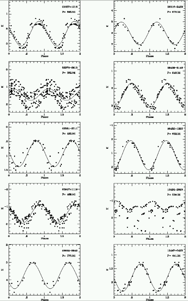
Figure 1: Phased Light-curves

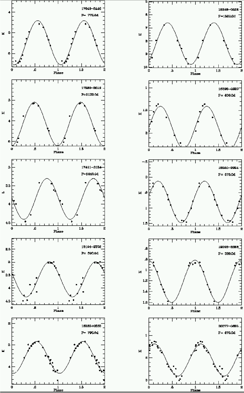
Figure 1: Phased Lightcurves…..continued.

$$M=\frac{{\Delta}M}{2}{\sin({\phi}-{\phi}_{0})}+M_{av}$$ (1)

where M is the magnitude in a particular band, ${\Delta}M$ the peak to peak amplitude, ${\phi}$ related to the phase, $p$, by ${\phi}=2{\pi}p$ and ${\phi}_{0}$ the phase angle at zero phase. $M_{av}$ is the mean magnitude.

One immediate observation from most of the phased light-curves is that at a given phase there is a range of magnitudes, rather than one sharply defined magnitude. This is not, in general, due to observational error, but is contributed to by various effects. First, Miras and OH/IR stars are erratic pulsators in the sense that their light curves do not exactly repeat from one cycle to the next at visual or infrared wavelengths (Koen & Lombard 1995; Whitelock, Marang & Feast 2000) Secondly, some stars, particularly carbon stars go through faint phases from time to time due to variable dust obscuration, e.g. $02270-2619$ (R For, see Whitelock et al 1997a). Thirdly, a very small number of stars show temporal or long term changes in luminosity, amplitude and/or period, possibly due to evolutionary effects (Whitelock 1999 and references therein).

Many of the light curves in Fig. 1 show clear departures from simple sinusoids and would be better fitted by the inclusion of one or two harmonics, in particular, $09429-2148$ and $12447+0425$. The most strikingly odd curve is that of $10491-2059$ (V Hya) which is discussed below.

4.1.1 V Hya

V Hya is a well studied carbon star and semi-regular variable. It has a bipolar circumstellar outflow, and models invoke rotation of the central star or the presence of a binary companion to explain bipolar outflows (Barnbaum, Morris & Kahane 1995).

Fig. 2a illustrates the light curve for V Hya using $K$ magnitudes measured from SAAO, including material from Lloyd Evans (1997 and private communication) together with the data from Table 2. In addition to the regular pulsation V Hya experienced two faint phases around JD 244 3500 and 244 9500. A Fourier analysis of the $K$ data when the star is bright, between JD 244 6000 and 244 8250 provide a period of 530 days, identical to the value given in the GCVS. Fig. 2b shows the data phased at this period and illustrates the double peak caused by harmonics in the light curve.

Figure 2: (a) $K$ light curve of V Hya. (b) data between JD 244 6000 and 244 8250 phased at 530 days.

Knapp et al. (1999) analysed 3260 AAVSO visual magnitude estimates covering almost 35 years. They confirm and refine the very long period found by Mayall (1965) at $6160\pm 400$ days. The two faint phases seen in Fig. 2a are consistent with this long period. The amplitudes of these 6160 day variations are at least 2.4, 2.1, 1.7 and 0.7 mag, at $JHKL$, respectively, while $\Delta V\sim 3.5$ mag (Knapp et al. 1999).

Barnbaum et al. (1995) found evidence for rapid rotation in V Hya, using spectral line broadening analysis. They suggest that the long term variation can be attributed to a coupling between the radial pulsation, with period of 530 days, and the rotation of the star with a very similar period. It is not clear how this interaction would give rise to the very long period without strongly modulating the shorter period, or why it should result in the observed reddening of the star during the faint phases.

Lloyd Evans (1997) suggested that the long period may be the result of obscuration events like those observed in R For. Although the colours would be consistent with this, the regularity of the long period (Knapp et al. 1999) is quite unlike the effect observed in R For and this explanation therefore seems unlikely.

Knapp et al. (1999) on the other hand, suggest that the long-period dimming of this star is due to a thick dust cloud orbiting the star and attached to a binary companion. Indeed, there is evidence for large numbers of late-type binaries in the LMC (Wood et al. 1999), so this may not be rare occurrence. The colour variations of V Hya are less extreme than those expected from optically thin interstellar dust, but they could be explained by large particles.

4.2 Period Distributions

The period distributions for the oxygen- and carbon-rich stars are plotted in Fig. 3. Most of the stars in the sample have periods between 500 and 700 days and almost all have periods between 300 and 900 days. There are only three extreme OH/IR stars with periods in excess of 1000 days. Fig. 3 can be compared with Whitelock et al. (1994) fig. 8 which shows the period distribution of IRAS selected Miras in the South Galactic Cap. Most of the Cap sample have $150<P<450$ days, i.e. shorter than the sample under discussion, but longer than optically selected Miras. Longer period Miras have more massive progenitors and are therefore lower scale heights. It is not surprising to find more of them in the solar neighbourhood than in the Galactic Cap.

A comparison of the period distributions of the oxygen- and carbon-rich stars is instructive. There are no carbon-rich stars with periods longer than 1000 days. From Fig. 3 it can be seen that the maximum of the carbon-star period distribution seems to be slightly shifted to longer periods than that of the oxygen-rich stars. A Kolmogorov-Smirnov (KS) test, when applied to these two distributions for periods less than 1000 days, yields a probability that the two distributions come from the same parent population of $0.40$. This probability ($>0.05$) implies that there is no significant difference in the period distributions for the carbon- and oxygen-rich stars.

The KS test cannot be used if the very long period stars are included since it is not very sensitive to differences in the tails of the distributions, as is well known. In this case the F-test and then the appropriate version of the student t-test is applied. The F-test gives a probability that the variances of the two distributions are the same of $2.5\times 10^{-5}$, i.e. very unlikely, which is obvious from Fig. 3. The appropriate version of the t-test, which takes differences in variances into account, gives a probability that the two distributions have the same mean of $0.24$. This probability ($>0.05$) implies that there is no statistical evidence for any difference in the mean of the two distributions.

Figure 3: Period distributions

4.3 Amplitudes

Table 5 lists the stars for which periods were determined together with their amplitudes, from equation 1, at $JHKL$. These amplitudes are plotted against period in Fig. 4, where a clear correlation can be seen at all wavelengths.

Figure 4: Light-Amplitude vs. pulsation period, the lines show least squares fits; filled and open circles represent carbon- and oxygen-rich stars, respectively.

The amplitude clearly decreases with wavelength (see also Feast et al. 1982). Quantitatively, the average amplitudes, relative to that at $J$ are, for $H$, $K$ and $L$ respectively, $0.84\pm 0.1$, $0.69\pm 0.14$ and $0.59\pm 0.14$. The linear correlation coefficient between the average relative amplitude and wavelength is $-0.93$ with a correlation probability of $Prob=0.07$ (using the relative amplitude at $J$ of $1$). This probability is considered as marginally significant. The KS test gives the probability for the null hypothesis that the light amplitude distributions for the carbon- and oxygen-rich stars (with $P<1000$ days) came from the same parent population at $J$, $H$, $K$ and $L$ of 0.25, 0.92, 0.51 and 0.52 respectively. Hence there is no statistical reason to suspect that these carbon- and oxygen-rich stars have significantly different light-amplitudes in the near-infrared.

5 Colours

5.1 Average Colours

Average near-infrared colours, i.e. consisting of $JHKL$ magnitudes only, were calculated for each star using the magnitudes at the dates of minimum and maximum $K$-light. This average is compared to a Fourier-fit colour in Appendix A. The two values are quite comparable with mean differences for all the near-infrared colours not exceeding 0.1 mag. Note that due to the very small phase coverage of $17411-3154$ in the $K$-band, the derived $K-L$ colour of this star may not be a good representative of the average $K-L$ colour.

The IRAS colours were obtained using the data in Table 4, where the colour-corrected IRAS fluxes were converted to magnitudes using the zero points listed in the IRAS-ES. Colours consisting of $JHKL$ and IRAS photometry, were calculated by combining average magnitudes in the $JHKL$ bands (Table 3) with the IRAS magnitudes.

For the northern sources and the three non-IRAS sources the average $K$ magnitudes were taken from Table 3, to calculate the $K-[12]$ colour. For the non-IRAS (carbon-rich) sources the average $12\mu$m magnitudes were estimated from the average $[11]-[12]=0.1\pm 0.3$ colour for the carbon-rich sources and the 11$\,\mu$m magnitudes listed in Table 4. All the derived infrared colours are given in Table 6.

Table 6: Infrared Colours

$\bf NAME$	$\bf J-H$	$\bf H-K$	$\bf J-K$	$\bf K-L$	$\bf K-[12]$	$\bf[12]-[25]$	$\bf[25]-[60]$
IRAS $00042+4248$					$5.37$	$1.06$	$0.04$
IRAS $01037+1219$	$3.51$	$2.26$	$5.77$	$2.48$	$6.26$	$1.21$	$0.25$
IRAS $01159+7220$					$4.65$	$0.96$	$-0.22$
IRAS $02270-2619$	$1.71$	$1.33$	$3.04$	$1.47$	$3.54$	$0.19$	$0.24$
IRAS $02316+6455$					$5.87$	$1.07$	$-0.16$
IRAS $02351-2711$	$1.25$	$0.69$	$1.94$	$0.79$	$3.66$	$0.86$	$-0.32$
IRAS $03229+4721$					$4.60$	$0.42$	$0.18$
IRAS $03507+1115$	$1.96$	$1.16$	$3.12$	$1.32$	$4.81$	$0.68$	$-0.27$
IRAS $04307+6210$					$3.90$	$0.42$	$0.12$
IRAS $04566+5606$					$3.69$	$0.45$	$0.23$
IRAS $05073+5248$					$5.22$	$1.56$	$0.41$
IRAS $05411+6957$					$4.30$	$0.84$	$-0.27$
IRAS $05559+7430$					$3.36$	$0.79$	$-0.03$
IRAS $06176-1036$	$1.66$	$1.58$	$3.24$	$2.11$	$6.43$	$1.40$	$0.78$
IRAS $06300+6058$					$3.48$	$1.06$	$0.22$
IRAS $06500+0829$					$4.34$	$0.82$	$0.54$
IRAS $08088-3243$	$2.59$	$2.12$	$4.71$	$2.62$	$6.37$	$0.60$	$0.18$
IRAS $09116-2439$		$3.75$		$3.56$	$9.40$	$0.78$	$0.20$
IRAS $09429-2148$	$1.86$	$1.34$	$3.19$	$1.62$	$5.39$	$1.30$	$-0.16$
IRAS $09452+1330$	$3.20$	$2.82$	$6.02$	$3.74$	$9.09$	$0.64$	$0.37$
IRAS $10131+3049$	$2.70$	$2.15$	$4.85$	$2.61$	$6.24$	$0.38$	$0.29$
IRAS $10491-2059$	$1.79$	$1.27$	$3.06$	$1.55$	$3.69$	$0.51$	$0.24$
IRAS $12447+0425$	$1.85$	$1.29$	$3.15$	$1.54$	$3.80$	$0.22$	$0.17$
IRAS $17049-2440$		$3.04$		$3.62$	$9.02$	$0.90$	$0.33$
IRAS $17119+0859$	$1.42$	$1.08$	$2.50$	$1.57$	$5.10$	$1.18$	$-0.28$
IRAS $17297+1747$	$3.04$	$2.33$	$5.37$	$2.93$	$6.73$	$1.13$	$0.04$
IRAS $17360-3012$	$3.01$	$2.07$	$5.08$	$2.43$	$6.28$	$1.79$	$0.26$
IRAS $17411-3154$				$6.25$	$13.99$	$2.14$	$1.04$
IRAS $18009-2019$	$1.73$	$1.02$	$2.74$	$1.01$	$3.78$	$1.11$	$-0.07$
IRAS $18040-0941$	$2.46$	$1.74$	$4.20$	$1.95$	$4.43$	$0.45$	$0.36$
IRAS $18194-2708$	$3.20$	$2.39$	$5.59$	$2.80$	$7.06$	$0.40$	$0.45$
IRAS $18240+2326$		$3.24$		$3.93$	$9.21$	$0.92$	$0.14$
IRAS $18333+0533$	$4.26$	$2.48$	$6.74$	$2.44$	$6.25$	$1.44$	$0.32$
IRAS $18348-0526$				$6.27$	$11.19$	$1.94$	$1.44$
IRAS $18349+1023$	$1.55$	$0.90$	$2.45$	$1.09$	$3.98$	$0.58$	$0.20$
IRAS $18397+1738$	$2.14$	$1.74$	$3.88$	$2.12$	$4.92$	$0.56$	$0.40$
IRAS $18398-0220$	$2.40$	$1.72$	$4.12$	$1.98$	$4.83$	$0.57$	$0.23$
IRAS $18413+1354$	$1.81$	$0.97$	$2.78$	$0.98$	$3.97$	$1.13$	$-0.19$
IRAS $18560-2954$	$1.47$	$0.84$	$2.31$	$1.07$	$3.99$	$0.76$	$0.12$
IRAS $19008+0726$	$2.63$	$2.04$	$4.67$	$2.45$	$5.38$	$0.49$	$0.20$
IRAS $19059-2219$	$1.72$	$1.04$	$2.77$	$1.12$	$4.45$	$1.15$	$-0.07$
IRAS $19093-3256$	$1.31$	$0.70$	$2.01$	$0.76$	$3.61$	$1.02$	$-0.08$
IRAS $19126-0708$	$1.31$	$0.79$	$2.10$		$4.61$	$0.60$	$-0.02$
IRAS $19175-0807$	$2.70$	$2.04$	$4.74$	$2.46$	$5.46$	$0.67$	$0.38$
IRAS $19321+2757$	$2.42$	$1.89$	$4.31$	$2.29$	$5.06$	$0.73$	$0.30$
IRAS $20077-0625$	$2.89$	$1.90$	$4.79$	$1.98$	$6.13$	$1.24$	$0.16$
IRAS $20396+4757$					$3.60$	$0.35$	$0.22$
IRAS $20440-0105$	$1.18$	$0.56$	$1.74$	$0.65$	$3.16$	$0.89$	$-0.14$
IRAS $20570+2714$	$2.96$	$2.43$	$5.39$	$2.88$	$5.83$	$0.76$	$0.22$
IRAS $21032-0024$	$1.92$	$1.35$	$3.27$	$1.51$	$3.71$	$0.44$	$0.14$
IRAS $21286+1055$	$1.38$	$0.86$	$2.24$	$1.01$	$3.48$	$1.04$	$0.00$
IRAS $21320+3850$					$3.75$	$0.38$	$0.26$
IRAS $21456+6422$					$3.17$	$0.99$	$-0.10$
IRAS $23166+1655$				$6.23$	$14.05$	$1.43$	$0.61$
IRAS $23320+4316$					$7.23$	$0.66$	$0.34$
IRAS $23496+6131$					$4.98$	$1.08$	$0.03$
RAFGL $1406$					$5.1$
RAFGL $2688$					$11.1$

5.2 Colour-Colour Diagrams

Infrared two colour diagrams are illustrated in Figs. 5 to 8. There is a clear separation of the oxygen- and carbon-rich stars in these diagrams with the carbon stars falling to the lower right of the oxygen-rich stars in the near-infrared two colour diagrams (Figs. 5 and 6) and to the left of them in the combined diagram, Fig. 7. The $JHKL$ colours of these AGB stars are more extreme than those of the well studied Miras (e.g. Feast et al. 1982), or even of IRAS selected Miras in the Galactic Cap (Whitelock et al. 1994).

Figure 5: $J-H$ versus $H-K$; filled circles represent carbon-rich stars, open circles oxygen-rich stars and five-point star S-type stars. The solid line represent loci of blackbodies of different temperatures.

Figure 6: J-K versus K-L. Symbols as in Fig. 5.

5.2.1 The $K-[12]$ versus $[12]-[25]$ Diagram

Of particular interest is the $K-[12]$ vs. $[12]-[25]$ diagram (Fig. 7). The colours of the oxygen- and carbon-rich stars separated rather clearly in this diagram. This has been noted previously (Le Bertre et al. 1994) and shown to be the result of the difference in the ratios of the near-infrared to mid-infrared opacities for the carbon- and oxygen-rich dust.

The single carbon star which falls among the oxygen-rich stars is $06176-1026$ (the Red Rectangle), a well studied, but peculiar star. It has an IRAS LRS classification of $80$ indicating the presence of the $11.3\mu$m line in emission in contrast to the other carbon stars which show $11.3\mu$m absorption, hence its position in Fig. 7. It is thought to be a pre-planetary nebula with an oxygen-rich circumstellar disk (see section 2.1).

Figure 7: K-[12] versus [12]-[25]. Symbols as in Fig. 5. Dotted line separates the chemical types and is given by equation 3.

The dashed line in Fig. 7 has been positioned so as to separate the carbon- and oxygen-rich stars as far as possible, it is described by:

$$(K-[12])=11.5([12]-[25])-3.8$$ (2)

Thus if we define ${\delta}_{C/O}$ as follows:

$${\delta}_{C/O}=11.5([12]-[25])-(K-[12])-3.8,$$ (3)

The two chemical types can be separated by a single parameter, ${\delta}_{C/O}$, such that for carbon stars ${\delta}_{C/O}<0$ and for most oxygen-rich stars ${\delta}_{C/O}>0$. This parameter might be useful for separating these objects over the colour range discussed. On this sample, obviously the one used to define the parameter, only 6 percent of stars were misclassified.

The two S-type stars were omitted from the above discussion, we note that one of them falls with the carbon- and the other with the oxygen-rich stars.

5.2.2 IRAS Two Colour Diagram

Van der Veen & Habing (1988) demonstrated that the position of an AGB star in an IRAS two-colour diagram, of the type shown in Fig. 8, was indicative of its chemical type and the thickness of its dust shell. Combined with information on variability and IRAS spectral-type the diagram provides a useful diagnostic. The colour indices for this plot ($C_{12/25}$, $C_{25/60}$) are defined by:

$$C_{12/25}=2.5\log({\frac{F_{25\mu{m}}}{F_{12\mu{m}}}}),$$

$$C_{25/60}=2.5\log({\frac{F_{60\mu{m}}}{F_{25\mu{m}}}}),$$

where the IRAS fluxes are not colour corrected.

Figure 8: $C_{25/60}$ versus $C_{12/25}$. Symbols as in Fig. 5. $18135-1641$ has only an upper limit to its $C_{25/60}$ colour as indicated by the arrow.

Following van der Veen & Habing the diagram is divided into regions, each of which is dominated by a certain type of object. Stars with low mass-loss rates will fall in the lower left of the diagram and increasingly higher mass-loss rates are found as one moves to the upper right.

Most of the oxygen-rich stars under discussion occupy region IIIa which van der Veen & Habing found to contain variable stars with moderate oxygen-rich dust-shells. Four stars are located in regions IIIb and IV, indicating thick to very thick oxygen-rich dust-shells and high mass-loss rates. Four oxygen-rich stars are located in region VII, an area dominated by carbon stars, but where van der Veen & Habing also found oxygen-rich stars.

Most of the LRS spectra for oxygen-rich stars in this sample are classified as 2n, indicating that the $10\mu$m silicate feature is in emission. The two oxygen-rich variables with the reddest $[12]-[25]$ colour, $17411-3154$ and $18348-0526$, have LRS classifications of 3n, i.e. their spectra show the $10\mu$m silicate feature in absorption. In these stars the dust-shell has become so cool and optically thick that the silicate feature has gone into absorption.

Most of the carbon-stars fall in region VII, which is characterised by variable stars with well developed carbon-rich dust-shells. All of these stars have an LRS classification of 4n, indicating that the SiC $11\mu$m feature is in emission. The Red Rectangle, $06176-1036$, (discussed above) is located in region IIIa, as is $23166+1655$. The latter object has an LRS classification of O2, probably due to self absorption of the SiC feature in the very think shell (Loup et al. 1993).

6 Bolometric Magnitudes and Distances

6.1 Apparent Bolometric Magnitudes

Given that these sources were selected on the basis of their high fluxes and therefore small distances, together with the fact that the bulk of their energy is emitted at infrared wavelengths it is reasonable to assume that the effects of interstellar extinction are negligible. The apparent bolometric magnitude, $m_{bol}$, were calculated by integrating under a spline curve (Hill 1982), fitted to the $J$, $H$, $K$, $L$, 12- and 25-$\mu{m}$ fluxes as a function of frequency. The end-points were dealt with by extrapolating a line, which joins the $J$ flux and the point lying halfway between the $H$ and $K$ fluxes, to zero flux. Zero flux at zero frequency was assumed. The derived values of $m_{bol}$ are listed in Table 7 for the sources with sufficient photometry.

For the very red sources $23166+1655$ and $18348-0526$, which have no measurements in the $J$ and/or $H$ bands, zero flux at $J$ and $H$ was assumed when making the spline fit.

To estimate an upper-limit to the amount of flux not accounted for by ignoring the tail in the flux distribution, a Wien approximation, ${\sim}A{\nu}^{3}e^{-b{\nu}}$ (where A and b are constants), was assumed for flux at frequencies higher than $J$ with the same slope as the spline at $J$. In more than 75 percent of the cases the difference between the fluxes calculated in this way and the simple spline fit was less than 1 percent. $20440-0105$, which has the smallest $K-[12]=3.16$, shows the maximum difference of 5 percent. Neglecting $\rm H_{2}O$ absorption between the $J$,$H$,$K$ and $L$ bands (Robertson & Feast 1981) will have a negligible effect on the bolometric magnitude estimated for stars whose flux originates largely from the circumstellar dust-shell.

Figure 9: $BC_{12}$ versus $K-[12]$. Symbols as in Fig. 5. Curves are those given in equations 4 and 4.

The bolometric corrections at 12$\,\mu{m}$, $BC_{12}$, is plotted against the $K-[12]$ colour in Fig. 9, together with curves given by:

$$BC_{12}=-15.4{e^{-0.70(K-[12])}}+8.10,$$ (4)

and

$$BC_{12}=-7.59{e^{-0.43(K-[12])}}+8.41,$$ (5)

which are least-square fits of this form to the oxygen- and carbon-rich star data respectively. The rms difference between the data and these curves is 0.04 and 0.06 mag respectively. For the remaining sources $m_{bol}$ was calculated from [12] and $K-[12]$ using equations 4 and 5.

The apparent luminosities derived here are typically rather smaller than those estimated by JK89, because of the colour corrections applied to the IRAS photometry.

6.2 Absolute Bolometric Magnitudes and Luminosities

For the 47 stars with periods the absolute bolometric magnitudes, $M_{bol}$, was calculated from the period-luminosity (PL) relation, equation 6, derived for LMC variables (Feast et al. 1989) assuming an LMC distance modulus of 18.60 mag (Whitelock et al. 1997b) and the results given in Table 7.

$$M_{bol}=-2.34\log P+1.26$$ (6)

The average luminosity, for all stars with periods less than 1000 days is $(0.98\pm 0.17)\times 10^{4}\,L_{\odot}$, or $M_{bol}=-5.23\pm 0.19$. For stars with unknown periods this mean value is assumed; which seems reasonable since the carbon stars seem to have periods less than 1000 days and the remaining oxygen-rich stars have $[12]-[25]$ colours suggesting that they too have periods less than a 1000 days. This value of the mean luminosity suggests that the $10^{4}L_{\odot}$ often assumed for the luminosity of the tip of the AGB is consistent with the application of the PL relation to this type of AGB star. Note this value may not be applicable to the Red Rectangle and the Egg Nebula, since they may have left the AGB already.

It is not really clear at this stage how well the various PL relations fit long period variables or if different relations should be used for the oxygen- and carbon-rich stars. Provided this caveat is born in mind when the results are interpreted it seems reasonable to use the luminosities derived as described above.

Note, in particular, that the PL relation used above was derived for stars with periods less than 420 days and it may not be appropriate to use it for the present sample. There certainly are long period AGB ($P>420$ days) stars in the LMC that lie above the PL relation (e.g. Feast et al. 1989). However, recent work on dust-enshrouded stars in the LMC suggest that these AGB stars are over-luminous because they are undergoing hot bottom burning and that more normal long period ($P\geq 400$ day) carbon- and oxygen-rich AGB stars fall very close to the PL derived for shorter period oxygen-rich stars (Whitelock & Feast 2000).

6.3 Distances

Distances to all the stars in the sample (excluding the Red Rectangle and the Egg Nebula) were calculated from $m_{bol}$ and $M_{bol}$ and are listed in Table 7. These distances are typically larger than those estimated by JK89. As discussed above the apparent luminosities used here are smaller than JK89’s, while the absolute luminosities are on average the same, except for the 3 stars with $P>1000$ where they are brighter. Thus we find sources with distances up to 2 kpc.

The other plausible way of estimating distances to OH/IR stars is the phase lag method, although it is notoriously difficult and time consuming. Van Langevelde, van der Heiden & Schooneveld (1990) measured phase lag distances for two of the stars under discussion. For $01037+1219$ (WX Psc) they get $0.74\pm 0.15$ kpc, identical to the PL distance given in Table 7. For $18348-0526$ (OH26.5+0.6) they give two values, $1.44\pm 0.27$ and $1.30\pm 0.35$ kpc, both somewhat closer than the 1.9 kpc listed in Table 7. Given the uncertainties in phase lag and the PL method this difference is not problematic. West (1998) has measured a phase lag distance for $17411-3154$ (OH357.3–1.3) of $1.2\pm 0.4$ kpc, in agreement with the distance of 0.99 kpc listed in Table 7.

Figure 10: $\bar{\lambda_{10}}$ versus $K-[12]$. Filled and open circles represent carbon- and oxygen-rich stars, respectively. The arrowed point, the Red Rectangle, is not used in the solution.

7 Mass-loss rates

Mass-loss rates, $\dot{M}$, were $estimated$ using the expression given by Jura (1987):

$$\dot{M}=1.7\times 10^{-7}v_{15}r^{2}_{kpc}L^{-1/2}_{4}F_{\nu,60}{\bar{\lambda}}_{10},$$ (7)

where $v_{15}$ is the outflow velocity of the gas in units of 15 $\rm km\,s^{-1}$, $r_{kpc}$ the distance to the star in kpc, $L_{4}$ the luminosity in units of $10^{4}L_{\odot}$, $F_{\nu,60}$ the flux measured at $60\mu$m in Jansky and ${\bar{\lambda}}_{10}$ the mean wavelength of light emerging from the star and its circumstellar dust-shell in units of $10\mu$m.

Equation 7 assumes all the grains have an emissivity of $\rm 150\,cm^{2}g^{-1}$ at $60\mu$m and a dust to gas ratio of $4.5\times 10^{-3}$ (Jura 1986). The mean wavelength of light emerging from the star and its circumstellar dust-shell, $\bar{\lambda}_{10}$, is given by:

$$\bar{\lambda}_{10}=\frac{\int_{0}^{\infty}{\lambda}{F_{\lambda}}d{\lambda}}{\int_{0}^{\infty}{F_{\lambda}}d{\lambda}}$$ (8)

where $F_{\lambda}$ the monochromatic flux density in units of energy received per unit area per unit time per unit wavelength interval.

For the stars for which the function $F_{\nu}$ could be estimated (section 6.1), $\bar{\lambda}_{10}$ was calculated from equation 8 and is listed in Table 7. The relationship between ${\bar{\lambda}}_{10}$ and $K-[12]$ is illustrated in Fig. 10 and can be expressed as:

$${\bar{\lambda}}_{10}=c+b(K-[12])+a(K-[12])^{2},$$ (9)

where a, b and c are constants.

Least square fits of equation 9 to the data results in the following values (a,b,c) for oxygen-rich (–0.0110,0.284,–0.392) and carbon-rich (–0.0137,0.338,–0.513) stars, respectively, with an rms error of $0.05\,\mu$m for both chemical types. The discrepant carbon star is the Red Rectangle which was omitted from the solution.

Equation 9 with the appropriate parameters is used to estimate ${\bar{\lambda}}_{10}$ for the remaining stars in the sample; the results are listed in Table 7

The outflow velocities, $v_{15}$, were taken to be the expansion velocities of the shell obtained from CO($1\rightarrow 0$) line measurements. Appropriate values from the literature are listed in Table 7 with references. For the three stars without measurements an average outflow velocity, for stars with $v_{out}<25\,\rm km\,s^{-1}$, of $17\pm 4\,\rm km\,s^{-1}$ was used. Jones et al. (1983, henceforth JHG) have shown there to be a correlation between outflow velocity and luminosity for a sample of OH/IR stars (see fig. 1 in JHG). The outflow velocity versus luminosity for stars with periods in our sample is illustrated in Fig. 11. It shows no obvious correlation, which should not be entirely unexpected, considering the large spread in outflow velocity at a given luminosity (up to $10\,km\,s^{-1}$) in fig. 1 of JHG and the small range in $M_{bol}$ in Fig. 11 (compared to that in fig. 1 of JHG).

Table 7: Physical and Kinematic data.

$\bf{NAME}$	$\bf{m_{bol}}$	$\bf{M_{bol}}$	$\bf{D}$	$\bf{{\bar{\lambda}}_{10}}$	$\bf{v_{out}}$	$\bf{Log(\dot{M})}$	$\bf{Log({\dot{M}}_{model})^{*}}$	$\bf{v_{lsr}}$
			$\bf{(kpc)}$		$\bf{(km\,s^{-1})}$			$\bf{(km\,s^{-1})}$
IRAS $00042+4248$	$(4.89)$	$-5.51$	$1.20$	$(0.91)$	$21.7$	$-4.87$	$-4.62$	$-19.0$
IRAS $01037+1219$	$4.00$	$-5.35$	$0.74$	$1.06$	$21.6$	$-4.64$	$-4.92$	$-50.1$
IRAS $01159+7220$	$(5.16)$	$-5.30$	$1.24$	$(0.76)$	$21.4$	$-5.19$	$-5.46$	$9.9$
IRAS $02270-2619$	$4.64$	$-4.84$	$0.79$	$0.49$	$20.0$	$-5.82$	$-5.82$	$-68.1$
IRAS $02316+6455$	$(5.08)$	$-5.16$	$1.12$	$(1.00)$	$15.4$	$-5.10$	$-4.96$	$4.5$
IRAS $02351-2711$	$4.21$	$-5.05$	$0.71$	$0.51$	$16.2$	$-5.77$	$-5.59$	$-66.5$
IRAS $03229+4721$	$(4.39)$	$-5.17$	$0.82$	$(0.68)$	$15.3$	$-5.51$	$-5.26$	$-7.6$
IRAS $03507+1115$	$2.35$	$-5.03$	$0.30$	$0.79$	$22.0$	$-5.31$	$-5.35$	$-31.4$
IRAS $04307+6210$	$(4.87)$	$-5.23$	$1.05$	$(0.55)$	$18.8$	$-5.62$	$-5.10$	$9.9$
IRAS $04566+5606$	$(2.75)$	$-5.21$	$0.39$	$(0.55)$	$18.7$	$-5.59$	$-5.52$	$8.6$
IRAS $05073+5248$	$(5.44)$	$-5.33$	$1.43$	$(0.88)$	$18.0$	$-4.66$	$-5.24$	$7.8$
IRAS $05411+6957$	$(4.09)$	$-5.23$	$0.73$	$(0.69)$	$21.2$	$-5.37$	$-5.00$	$20.1$
IRAS $05559+7430$	$(4.77)$	$-5.14$	$0.96$	$(0.47)$	$15.1$	$-5.82$	$-5.85$	$22.9$
IRAS $06176-1036$	$4.99$			$1.17$	$01.6$			$-11.7$
IRAS $06300+6058$	$(4.33)$	$-5.23$	$0.82$	$(0.50)$	$16.8$	$-5.48$	$-5.26$	$21.5$
IRAS $06500+0829$	$(4.09)$	$-5.15$	$0.70$	$(0.70)$	$20.0$	$-5.08$	$-5.21$	$4.1$
IRAS $08088-3243$	$5.45$	$-5.23$	$1.37$	$0.98$	$20.7$	$-4.97$	$-5.20$	$0.4$
IRAS $09116-2439$	$4.94$	$-5.39$	$1.17$	$1.29$	$13.4$	$-4.84$	$-4.92$	$16.2$
IRAS $09429-2148$	$4.75$	$-5.35$	$1.05$	$0.97$	$14.0$	$-5.05$	$-5.43$	$23.3$
IRAS $09452+1330$	$0.38$	$-5.37$	$0.14$	$1.26$	$15.0$	$-4.79$	$-4.32$	$45.1$
IRAS $10131+3049$	$2.96$	$-5.35$	$0.46$	$0.93$	$16.9$	$-5.10$	$-5.12$	$56.0$
IRAS $10491-2059$	$3.04$	$-5.16$	$0.44$	$0.52$	$14.2$	$-5.74$		$33.6$
IRAS $12447+0425$	$4.93$	$-4.97$	$0.95$	$0.53$	$16.9$	$-5.82$	$-5.08$	$67.0$
IRAS $17049-2440$	$4.77$	$-5.54$	$1.15$	$1.29$	$20.7$	$-4.54$	$-4.54$	$9.3$
IRAS $17119+0859$	$4.97$	$-5.23$	$1.10$	$0.85$	$14.0$	$-5.26$		$-0.8$
IRAS $17297+1747$	$4.91$	$-5.14$	$1.02$	$1.06$	$17.0$	$-4.90$	$-4.80$	$25.3$
IRAS $17360-3012$	$5.65$	$-5.94$	$2.08$	$1.16$	$20.0^{\dagger}$	$-4.34$		$0.5$
IRAS $17411-3154$	$3.80$	$-6.17$	$0.99$	$1.58$	$20.5$	$-3.67$	$-5.06$	$-1.3$
IRAS $18009-2019$	$4.38$	$-5.23$	$0.84$	$0.59$	$17.0^{\ddagger}$	$-5.42$		$0.8$
IRAS $18040-0941$	$5.21$	$-5.23$	$1.22$	$0.64$	$22.0$	$-5.31$	$-4.92$	$5.3$
IRAS $18194-2708$	$4.80$	$-5.42$	$1.11$	$1.06$	$23.0$	$-4.77$	$-5.03$	$-6.2$
IRAS $18240+2326$	$4.92$	$-5.23$	$1.07$	$1.29$	$15.1$	$-4.80$	$-4.82$	$15.8$
IRAS $18333+0533$	$5.38$	$-5.57$	$1.55$	$1.09$	$20.0$	$-4.52$	$-4.80$	$6.0$
IRAS $18348-0526$	$5.13$	$-6.26$	$1.90$	$1.44$	$10.6$	$-3.89$		$0.6$
IRAS $18349+1023$	$3.81$	$-5.10$	$0.60$	$0.58$	$17.0$	$-5.52$	$-5.26$	$7.8$
IRAS $18397+1738$	$4.41$	$-5.12$	$0.81$	$0.72$	$15.6$	$-5.31$	$-5.04$	$10.0$
IRAS $18398-0220$	$4.42$	$-5.28$	$0.87$	$0.72$	$34.5$	$-5.00$	$-4.77$	$1.0$
IRAS $18413+1354$	$5.25$	$-5.26$	$1.27$	$0.64$	$18.5$	$-5.36$	$-5.19$	$8.0$
IRAS $18560-2954$	$3.98$	$-5.24$	$0.70$	$0.59$	$13.2$	$-5.55$	$-5.09$	$-14.7$
IRAS $19008+0726$	$4.80$	$-5.24$	$1.02$	$0.78$	$17.4$	$-5.28$	$-5.21$	$0.8$
IRAS $19059-2219$	$5.16$	$-5.12$	$1.14$	$0.75$	$22.2$	$-5.10$	$-4.89$	$-13.6$
IRAS $19093-3256$	$4.44$	$-4.82$	$0.71$	$0.51$	$15.0$	$-5.72$		$-18.4$
IRAS $19126-0708$	$3.36$	$-5.08$	$0.49$	$0.68$	$19.9$	$-5.39$	$-5.07$	$-8.5$
IRAS $19175-0807$	$4.91$	$-5.40$	$1.16$	$0.80$	$35.5$	$-4.77$	$-5.24$	$-10.0$
IRAS $19321+2757$	$4.96$	$-5.32$	$1.14$	$0.74$	$24.4$	$-5.04$	$-4.66$	$4.0$
IRAS $20077-0625$	$3.99$	$-5.40$	$0.76$	$1.11$	$16.0$	$-4.76$	$-4.89$	$-20.3$
IRAS $20396+4757$	$(3.58)$	$-4.92$	$0.50$	$(0.49)$	$13.7$	$-5.92$	$-5.52$	$3.8$
IRAS $20440-0105$	$4.58$	$-5.23$	$0.92$	$0.41$	$10.8$	$-6.05$	$-5.40$	$-25.8$
IRAS $20570+2714$	$5.31$	$-5.51$	$1.46$	$0.83$	$23.5$	$-4.94$	$-5.35$	$-12.0$
IRAS $21032-0024$	$4.55$	$-5.00$	$0.81$	$0.53$	$16.1$	$-5.77$	$-5.42$	$-29.6$
IRAS $21286+1055$	$5.10$	$-5.00$	$1.05$	$0.51$	$13.5$	$-5.72$	$-5.55$	$-28.2$
IRAS $21320+3850$	$(4.69)$	$-5.03$	$0.88$	$(0.52)$	$14.0$	$-5.80$	$-5.64$	$-9.4$
IRAS $21456+6422$	$(4.75)$	$-5.32$	$1.03$	$(0.42)$	$17.0$	$-5.77$		$21.0$
IRAS $23166+1655$	$4.72$	$-5.44$	$1.08$	$1.43$	$14.5$	$-4.37$	$-4.68$	$-40.4$
IRAS $23320+4316$	$(4.38)$	$-5.31$	$0.87$	$(1.09)$	$14.6$	$-4.95$	$-4.68$	$-17.1$
IRAS $23496+6131$	$(5.05)$	$-4.92$	$0.98$	$(0.83)$	$19.0$	$-5.11$		$-0.3$
RAFGL $1406$	$(4.45)$	$-5.23$	$0.86$	$(0.75)$	$10.9$	$(-5.14)$		$33.9$
RAFGL $2688$					$19.0$		$-3.85$	$-6.5$

${*}$ - model mass-loss rates taken from Loup et al. (1993).
Almost all stars have outflow velocities taken from Loup et al. (1993), with the following exceptions:
${\dagger}$ - outflow velocities taken from Jura & Kleinmann (1989);
${\ddagger}$ - average outflow velocity of stars with $v_{out}<25\rm\,km\,s^{-1}$.

Figure 11: A comparison of the mass-loss rates determined from equation 7 and listed in Table 7 with those given by Loup at al. ($\dot{M}_{model}$) in the top panel and a plot of outflow velocity versus luminosity in the bottom panel (symbols as in Fig. 10).

Figure 12: Log($\dot{M}$) versus $K-[12]$. Filled and open circles represent carbon- and oxygen-rich stars respectively. The curves are described by equation 10.

The mass-loss rates for 58 of the stars in the sample were calculated from equation 7 and are listed in Table 7 together with mass-loss rates, ${\dot{M}}_{model}$, taken from the compilation by Loup et al. (1993). Where ${\dot{M}}_{model}$ was determined from detailed models of the CO emission. A comparison of these values is illustrated in Fig. 11 which shows that they agree within a factor of 3. This is reasonable given the uncertainty in the various assumptions used to derive equation 7. $17411-3154$ does not appear in Fig. 11, it has an extremely high mass-loss rate, $\dot{M}>10^{-4}M_{\odot}yr^{-1}$, from equation 7, much higher than the value, $0.87\times 10^{-5}M_{\odot}yr^{-1}$, given in Loup et al. (1993). Kastner (1992) applies a revised model of circumstellar CO emission, and suggests that it is losing mass at a rate greater than $\dot{M}>10^{-5}M_{\odot}yr^{-1}$, consistent with the value derived here.

Fig. 12 shows the relationship between mass-loss rate and $K-[12]$ ($\dot{M}$ correlates with other colours, but none as strongly as this). This relation for Miras has been discussed by Whitelock et al. (1994) and Le Bertre & Winters (1998). A least squares fit can be made to the data in Fig. 12 assuming the form:

$$\log(\dot{M})=\frac{a}{(K-[12]+b)}+c,$$ (10)

where a, b and c are constants.

This results in values (a,b,c) for carbon- (–2.89, –1.79, –4.32) and oxygen-rich (–21.34, 3.00, –2.40) stars respectively with rms uncertainties of 0.14 and 0.16. This expression can then be used to estimate mass-loss rate for the RAFGL 1406, which appear in brackets in Table 7.

Figure 13: Mass-loss rate ($\dot{M}$) as a function of pulsation period ($P$).

Fig. 13 shows that there is a correlation between mass-loss rate and the period of pulsation. Some dependence of mass-loss rate on period might be introduced by using the PL relation to calculate the quantities $L_{4}$ and $r_{kpc}$ for equation 7. If we assume, for the sake of argument, that these sources are all the same luminosity, then use of the PL will result in a mass-loss/period dependence of the form $\dot{M}\propto P^{0.47}$, i.e. a much weaker effect than is actually seen. A correlation between period and mass-loss rate was also found by Whitelock et al. (1994).

The average mass-loss rate for stars in this sample is $\dot{M}\sim 1.5\times 10^{-5}M_{\odot}yr^{-1}$. Stars with $P>1000$ day (i.e. $[12]-[25]>1.7$) have $\dot{M}\sim 1.3\times 10^{-4}M_{\odot}yr^{-1}$ and stars with $P<1000$ day (i.e. $[12]-[25]<1.7$) have $\dot{M}\sim 0.87\times 10^{-5}M_{\odot}yr^{-1}$. It will be seen later that stars with $P>1000$ day probably have main-sequence masses greater that $4\,M_{\odot}$, while those with $P<1000$ day have main-sequence masses between 1 and $2\,M_{\odot}$. Thus intermediate mass stars lose mass an order of magnitude faster than do low mass-stars. The average mass-loss rates of carbon- and oxygen-rich (including S-type) stars are $\dot{M}\simeq(1.0\pm 1.0)\times 10^{-5}M_{\odot}yr^{-1}$ and $\dot{M}\simeq(2.0\pm 1.2)\times 10^{-5}M_{\odot}yr^{-1}$ respectively. This slight difference may be a consequence of assuming the same grain emissivity and gas to dust ratio, in equation 7, for the two chemical types. Within the limits of the assumptions used here, the mass-loss rates of the carbon and oxygen-rich stars are plausibly identical.

One of the stars in this sample, RAFGL 1406 (IY Hya), is a known super-lithium-rich carbon star (i.e. it has $\log\frac{n(Li)}{n(H)}>-8$) and it is estimated that about 2 percent of carbon-stars are of this type (Abia et al. 1993a). Furthermore there is evidence that these stars are currently important contributors to lithium in the Galaxy (Abia et al. 1995 and 1998).

Abia et al. (1993b) estimate a lithium production rate of $<{\dot{m}}_{7}>=4.5\times{10^{-14}}\,M_{\odot}yr^{-1}$ per carbon star with a return rate into the interstellar medium ${P}_{7}=1.9\times{10^{-9}}\,M_{\odot}pc^{-2}\,Gyr^{-1}$. The sample of stars they studied have a typical mass-loss rate of $2\times{10^{-7}}\,M_{\odot}yr^{-1}$, i.e. more than a order of magnitude less than the average mass-loss rate of carbon-rich DE-AGB stars. Note that Abia et al. (1993b) derive a average progenitor mass for the carbon stars in their sample of 1.2-1.6$\,M_{\odot}$, which is similar to the average progenitor mass estimated for this sample (see later). Assuming a super-lithium-rich carbon star to have a typical lithium abundance of $\log\frac{n(Li)}{n(H)}=-7$ (see fig. 3 in Abia et al. 1993a) we estimate a lithium production rate from carbon-rich DE-AGB stars of $1.3\times{10^{-13}}\,M_{\odot}yr^{-1}$ per carbon star, with the fraction of super-lithium-rich carbon stars in this sample taken to be 0.02. The total return rate of lithium by these stars into the interstellar medium is then about $1.0{\times}10^{-9}\,M_{\odot}pc^{-2}\,Gyr^{-1}$. This indicates that carbon-rich DE-AGB stars may contribute up to a third of the lithium in the Galaxy produced from carbon-rich AGB stars. However, granting the underlying assumptions and uncertainty in the numbers above, further investigation into the problem is necessary (see e.g. Abia et al. 1993b).

8 Scale-height, Progenitor Mass and Lifetime

8.1 Scale-height

Assuming the usually exponential distribution of stellar densities the number of stars per height interval, ${\rho}$, varies with distance from the galactic plane, $z$, as:

$${\rho}={\rho}_{0}e^{-|z|/H},$$ (11)

where ${\rho}_{0}$ is the density of stars at $z=0$ and $H$ is the scale-height. For such a population the average height, $\bar{|z|}$, is equal to the scale-height, $H$, provided the sample is reasonably complete (as JK89 suggest it is).

The sample of stars discussed here were necessarily selected from a limited region of the sky by JK98. Taking this into account we use only stars with $14^{\circ}<l<230^{\circ}$ and find that $H=235$ pc.

Figure 14: The function $f_{|z|}$ gives the fraction of stars with distances from the plane less than $|z|$. The curve is described by equation 12.

Alternatively, the fraction of stars, $f_{|z|}$, within a given $|z|$ of the galactic plane is given by:

$$f_{|z|}=1-e^{-|z|/H}.$$ (12)

$f_{|z|}$ is plotted in Fig. 14 for each 100 pc interval for the sample of stars with $14^{\circ}<l<230^{\circ}$. A curve of the form given by equation 12, fitted by least squares, is also shown. This fits the data very well (rms difference 0.03) and provides a scale-height of $H=236\pm 10$ pc, comparable to the estimate made above. This value will be used below as representative of the scale height of the sample.

8.2 Progenitor Mass

The scale height derived above can be used to estimate a typical progenitor mass for the AGB population. A comparison with Miller & Scalo (1979 - their table 1) indicates an average main-sequence mass $M_{i}\simeq 1.2M_{\odot}$ for the group under discussion, although it is difficult to estimate the uncertainty on this value.

An alternative approach uses the data in table 3 of Miller & Scalo (1979) which gives the number of main-sequence stars pc${}^{-2}(\log(M))^{-1}$, $\phi_{i}$, as a function of $\log(M)$. A maximum likelihood straight line fit to these data over the range $-0.14<\log(M)<0.92$ has a slope $\alpha=-4.20\pm 0.32$, a zero-point $\beta=1.20\pm 0.14$ and fits the data fairly well. Let $M_{lower}$ and $M_{upper}$ be the lower and upper progenitor mass limits respectively of the stars in this sample. Then it is straight forward to show that the average mass, $\bar{M}$, in $M_{\odot}$ is given by:

$$\bar{M}={\frac{\alpha}{\alpha+1}}{\frac{M_{upper}^{\alpha+1}-M_{lower}^{\alpha+1}}{M_{upper}^{\alpha}-M_{lower}^{\alpha}}}$$ (13)

To get an idea of the values of $M_{lower}$ and $M_{upper}$ the relation between $M_{lower}$, $M_{upper}$ and the $average$ scale-height $\bar{H}$ was investigated. $\bar{H}$, for a given mass range $[M_{lower},M_{upper}]$ is simply given by:

$$\bar{H}=\frac{\int_{M_{lower}}^{M_{upper}}H(M)dN(M)}{\int_{M_{lower}}^{M_{upper}}dN(M)}$$ (14)

where $H(M)$ is the scale-height as a function of mass $M$ (table 1 from Miller & Scalo), $dN(M)=\frac{\phi_{i}}{Mln(10)}dM$ the number of stars$\,\rm pc^{-2}$ in the infinitesimally small interval $dM$ centred around $M$.

Figure 15: The interdependence of lower and upper mass limits for different scale heights.

Assuming an average scale-height, ${\bar{H}}_{0}$, then for a given upper mass limit $M_{upper}$ equation 14 can be solved numerically for $M_{lower}$, since the functions $H(M)$ and $\phi_{i}$ are known. This was done for ${\bar{H}}_{0}=H=236$ pc. The resulting relation between $M_{lower}$ and $M_{upper}$ is plotted in Fig. 15, from which it is clear that for $M_{upper}>3M_{\odot}$, $M_{lower}$ has a constant value of $0.96M_{\odot}$.

Now since we expect to find dust envelope (DE) AGB main-sequence progenitors up to about $8M_{\odot}$ and since the value of $\bar{M}$, from equation 13, is relatively insensitive to the value of $M_{upper}$ if $\frac{M_{upper}}{M_{lower}}>3$, values of $M_{lower}=0.93M_{\odot}$ and $M_{upper}=8M_{\odot}$ will be assumed. It is important to note that the value of $\bar{M}$ is essentially proportional to the value of $M_{lower}$ and almost independent of $M_{upper}$ if $\frac{M_{upper}}{M_{lower}}>3$. Also when calculating the surface density of progenitors, it will be seen that this is very sensitive to the value of $M_{lower}$. Changing the assumed average scale-height to 216 pc or 256 pc (i.e. effectively changing the assumed scale-height by about $2\sigma$) gives values of $M_{lower}$, assuming $M_{upper}=8M_{\odot}$, of $0.99M_{\odot}$ and $0.86M_{\odot}$ respectively. Thus an error in $M_{lower}$ of $0.07M_{\odot}$ will be assumed. This then gives an average mass from equation 13 of $(1.22\pm 0.18)M_{\odot}$.

From the discussion above, an average scale-height of 236 pc implies a progenitor mass range starting from about $0.96\,M_{\odot}$ up to possibly $8\,M_{\odot}$. Hence using equation 18 (below), one can estimate the ratio of the number of stars in the mass range $2.0M_{\odot}<M_{i}<8.0\,M_{\odot}$ to the number of stars in the mass range $1.0M_{\odot}<M_{i}<2.0\,M_{\odot}$. This ratio is only 0.06. The three stars with periods greater than 1000 days have an average height above the galactic plane of $20\pm 2$ pc. This indicates that the progenitors of these stars were probably more massive stars, with $M_{i}>4.0M_{\odot}$, as can be seen from Miller & Scalo’s table 1. Interestingly the ratio of stars with $P>1000$ day to the rest of the sample (which are expected to have $P<1000$ day from their colours) is 0.05, comparable to the ratio calculated above. The ratio, from equation 18, of the number of stars in the mass range $0.93M_{\odot}<M_{i}<1.0\,M_{\odot}$ to the number stars in the mass range $1.0M_{\odot}<M_{i}<2.0\,M_{\odot}$ is about 0.4. Thus the majority of the stars in this sample have main-sequence masses in the range $1.0M_{\odot}<M_{i}<2.0\,M_{\odot}$.

Limited discussion in the literature also supports this conclusion. Thus Kahane et al. (2000) estimate the main-sequence progenitor of $09452+1330$, one of the stars in our sample, to be of low mass ($M_{i}\leq 2M_{\odot}$) by comparing the predictions from AGB stellar models of solar composition and various initial mass with the observed chlorine isotopic ratio in its circumstellar shell. Also Nishida et al. (2000) estimate the progenitor mass of three carbon-rich Miras, with $P>450$ day, in Magellanic Cloud clusters to be $1.5$-$1.6\,M_{\odot}$ by main-sequence isochrone fitting.

The velocity dispersion of the stars with $P<1000$ provides another indication of initial mass. Fifty three sources have velocities, relative to the local standard of rest, tabulated by Loup et al. (1993), they show a dispersion $\sigma=24\pm 2\,\rm km\,s^{-1}$. After correcting for galactic rotation, using the constants from Feast & Whitelock (1997), this reduces to $\sigma=19\pm 2\,\rm km\,s^{-1}$. Table 8 lists the velocity dispersions (calculated from table 2 of Delhaye 1965) and initial masses (from Allen 1973) for main-sequence stars between A0 and G5. The velocity dispersion thus indicates that the mean sample has $M_{i}<2\,M_{\odot}$, consistent with numbers given above.

Table 8: Initial Masses and Velocity Dispersions for Main-Sequence Stars

Sp (V)	A0	A5	F5	G0	G5
$\sigma$ ($\rm km\,s^{-1}$)	11	14	21	22	23
M ($M_{\odot}$)	3.2	2.1	1.3	1.1	0.9

Figure 16: The distribution of stars around the sun in the Galactic Plane. Open and closed symbols represent oxygen- and carbon- rich stars respectively.

8.3 Surface Density

Fig. 16 shows the surface distribution of the stars in the galactic plane, calculated from the distances derived previously. As can be seen, most of the stars (90 percent) are within $1.4$ kpc of the sun. There are very few in quadrant $IV$ due to positional selection effects in the original sample. The surface density, $\sigma_{i}$ in region $i$, $i=I,II,III$, was estimated from:

$$\sigma_{i}=\frac{N_{i}}{\frac{1}{4}\pi(1.0)^{2}}\hskip 14.22636pt\rm stars\,kpc^{-2}$$ (15)

where $N_{i}$ is the number of stars in a particular region $i$.

The average surface density, $\sigma_{DE-AGB}$ of DE-AGB stars in the solar neighbourhood was then estimated from:

$$\sigma_{DE-AGB}=\frac{2\sigma_{I}+\sigma_{II}+\sigma_{III}}{4}$$ (16)

where $\sigma_{I}\simeq\sigma_{IV}$, assuming symmetry about $l=0$.
Using equations 15 and 16 we find $\sigma_{DE-AGB}=15\pm 4$ $\rm stars\,kpc^{-2}$.

8.4 Lifetime

Assuming the average lifetime of stars in any given phase of evolution is proportional to the number of stars in that phase, it follows that:

$${\bar{\tau}}_{DE-AGB}=\frac{\sigma_{DE-AGB}}{\sigma_{MS}}{\bar{\tau}}_{MS}$$ (17)

where ${\bar{\tau}}_{DE-AGB}$ is the average lifetime of DE-AGB stars, ${\bar{\tau}}_{MS}$ and $\sigma_{MS}$ the average lifetime and surface density, respectively, of the progenitors of DE-AGB stars on the main-sequence.

From the linear relation between $\log(\phi_{i})$ and $\log(M)$ it is straight forward to show that $\sigma_{MS}$ in the mass range $[M_{lower},M_{upper}]$, is simply given by:

$$\sigma_{MS}=\frac{10^{\beta}}{\alpha{ln(10)}}[M_{upper}^{\alpha}-M_{lower}^{\alpha}]$$ (18)

where $\sigma_{MS}$ is in units of $\rm stars\,pc^{-2}$.
It is clear from equation 18 and the value of $\alpha$ that $\sigma_{MS}$ is very sensitive to the value of $M_{lower}$ and $\propto{M^{\alpha}}_{lower}$ if $\frac{M_{upper}}{M_{lower}}>3.0$. Using the upper and lower mass limits assumed above, gives $\sigma_{MS}=2.22\pm 0.76$ $\rm stars\,pc^{-2}$.

Miller & Scalo’s table 1 also gives $\log(\tau_{MS})$ as a function of $\log(M)$. ${{\bar{\tau}}_{MS}}$ is simply given by:

$${\bar{\tau}}_{MS}=\frac{\int_{M_{lower}}^{M_{upper}}\tau_{MS}(M)dN(M)}{\int_{M_{lower}}^{M_{upper}}dN(M)}$$ (19)

Equation 19 was integrated numerically with the above mass limits, giving ${\bar{\tau}}_{MS}=(5.5\pm 1.5)\times 10^{9}$  years. The errors above were estimated by changing the average scale-height (and hence $M_{lower}$) to 216 and 256 respectively.

Using equation 17 an average lifetime for the stars in this sample was estimated, giving ${\bar{\tau}}_{DE-AGB}=(3.7\pm 1.9)\times 10^{4}$  years. This value is in excellent agreement with lifetimes of similar stars at the tip of the AGB estimated by various other investigators (see Habing 1996 p. 183).

9 Evolutionary Status and Conclusions

The stars under discussion were selected to isolate high mass-loss, thick dust-shell AGB stars within the Solar Neighbourhood. This study indicates that the selection criteria employed were fairly successful in this respect. The $JHKL$ photometry, the IRAS two-colour diagrams and other published data prove that the majority of these sources are cool variable stars with moderate to high mass-loss rates.

As shown above most of these stars will have had a main-sequence progenitor with $1\leq M\leq 2$ $M_{\odot}$. While the average progenitor mass is $\sim 1.3M_{\odot}$. Using this average value and an empirical “initial/final mass”-relation (Weidemann 1987) an average final white dwarf mass can be estimated at $\sim 0.56M_{\odot}$.

Assuming the core masses of these stars are close to the final white dwarf mass, it is found that the thermal interflash period (${t}_{if}$) will be, ${t}_{if}\simeq 10^{5}$ years, using the core-mass interflash period relation given by Boothroyd & Sackmann (1988) (their equation 6 which is valid for solar composition). A more recent core-mass interflash period relation given by equation 11a of Wagenhuber & Groenewegen (1998) also suggests a thermal interflash period of ${t}_{if}\simeq 10^{5}$ years; this is provided there is no hot bottom burning and that the star has already undergone several helium shell flashes (see Wagenhuber & Groenewegen). The first assumptions is reasonable as stars under 2 $M_{\odot}$ do not experience hot bottom burning. The second is also an essential assumption for using the final white dwarf mass for the current core mass and obviously the carbon stars, at least, have undergone several flashes.

This interflash period, ${t}_{if}\simeq 10^{5}$, is more than a factor of two larger than the average lifetime of these DE-AGB stars, $\bar{{\tau}}_{DE-AGB}=(3.7\pm 1.9)\times 10^{4}$ years, deduced above. Hence we can conclude that these DE-AGB stars will experience at most one thermal pulse before leaving the TP-AGB phase.

The average mass-loss rate, ${\dot{M}}_{ave}$ for stars in the sample was found to be $\sim 1.5\times 10^{-5}M_{\odot}yr^{-1}$. Thus the total mass lost, $M_{lost}$, by an average star in this phase is $M_{lost}={\dot{M}}_{ave}\bar{{\tau}}_{DE-AGB}\sim 0.5M_{\odot}$. Which is very close the average initial-final mass difference for these stars. However, this value for $M_{lost}$ is very uncertain due to the uncertainty in the mass-loss rates. Nevertheless, this indicates that a significant fraction of the envelope mass is lost during this high mass-loss dust-enshrouded TP-AGB phase.

The total rate of mass returned into the interstellar medium, ${\dot{M}}_{ISM}$, by stars in this phase is ${\dot{M}}_{ISM}={\dot{M}}_{ave}{\sigma}_{DE-AGB}\sim 2.3\times 10^{-4}M_{\odot}\,kpc^{-2}\,yr^{-1}$. Jura & Kleinmann (1990) estimate that M supergiants in the solar neighbourhood return mass to the interstellar medium at only a rate between $1\times 10^{-5}$ and $3\times 10^{-5}M_{\odot}\,kpc^{-2}\,yr^{-1}$. Thus AGB stars must be important contributors of material to the interstellar medium in the solar neighbourhood.

Acknowledgements

We would like to thank Chris Koen, Michael Feast and Peter Wood for helpful discussions and advice, Luis Balona for his Fourier analysis program and Tom Lloyd Evans for allowing us to use observations in advance of publications. We are also grateful to, Robin Catchpole and Dave Laney for making near-infrared observations on our behalf. This paper made use of the SIMBAD database and observations made from the South African Astronomical Observatory.

Appendix
Average Magnitudes and Colours

Average Magnitudes

For variable stars, such as those discussed here, it is often useful to know the average magnitude at a particular wavelength. The average magnitude as discussed in section 3, was taken as the mean of the minimum and maximum magnitude measured for the particular star. This average, $A_{M}$, is compared in Table A1 with the average magnitude, $\bar{M}$, derived from the fit given by equation 4.1 for the 19 stars with sufficient data. The average absolute difference, ${\Delta}_{M}$, between these two averages, for each near-infrared band, with the sample standard deviation, ${\sigma}_{\Delta}$, on this average is also listed in Table A1. From these values for ${\Delta}_{M}$ it can be seen that $A_{M}$ represents the average magnitude fairly well. Obviously in instances where there are insufficient observations to cover a complete cycle, $A_{M}$ will be a poor representation of the mean.

Average Colours

The stars in this sample not only vary in light output, but also in colour. In section 5 the average colour of a star is taken as the mean of the value calculated at each Julian Date, $A$. This average is then compared to the average colour, $A_{f}$, derived from the Fourier fits given by equation 4.1. $A_{f}$ is simply given by:

$$A_{f}=<M_{1}-M_{2}>=<M_{1}>-<M_{2}>={M}_{1,av}-{M}_{2,av}$$ (20)

where $M_{1}$ and $M_{2}$ are the magnitudes in the bands making up the colour. ${M}_{1,av}$ and ${M}_{2,av}$ are the average magnitudes in these bands obtained from the Fourier fits given by equation 4.1.

Both the averages, for each near-infrared colour, are listed in Table A2 for the 18 stars with sufficient data. Also listed in the Table are the average absolute difference, ${\Delta}_{A}$ and sample standard deviation, ${\sigma}_{\Delta}$, on this average. The two values are quite comparable.

Table 9: Average magnitudes for variable sources with with good phase coverage

$\bf{NAME}$	$\bf{J}$		$\bf{H}$		$\bf{K}$		$\bf{L}$
$\bf{(IRAS)}$	$\bf{\bar{M}}$	$\bf{A_{M}}$	$\bf{\bar{M}}$	$\bf{A_{M}}$	$\bf{\bar{M}}$	$\bf{A_{M}}$	$\bf{\bar{M}}$	$\bf{A_{M}}$
$01037+1219$	$7.84$	$8.06$	$4.57$	$4.71$	$2.34$	$2.32$	$-0.08$	$-0.09$
$02270-2619$	$4.54$	$4.57$	$2.77$	$2.74$	$1.43$	$1.42$	$-0.04$	$-0.06$
$02351-2711$	$2.75$	$2.92$	$1.57$	$1.67$	$0.93$	$0.98$	$0.17$	$0.19$
$03507+1115$	$2.23$	$2.57$	$0.47$	$0.69$	$-0.59$	$-0.47$	$-1.83$	$-1.79$
$08088-3243$	$8.45$	$8.57$	$5.87$	$5.97$	$3.77$	$3.86$	$1.19$	$1.24$
$09116-2439$			$9.40$	$9.68$	$6.03$	$6.04$	$2.15$	$2.22$
$09429-2148$	$5.50$	$5.65$	$3.75$	$3.69$	$2.40$	$2.36$	$0.72$	$0.73$
$09452+1330$	$7.26$	$7.28$	$3.98$	$3.99$	$1.15$	$1.17$	$-2.54$	$-2.55$
$12447+0425$	$4.89$	$4.88$	$3.13$	$3.08$	$1.83$	$1.81$	$0.28$	$0.26$
$17049-2440$			$8.50$	$8.57$	$5.47$	$5.51$	$1.88$	$1.93$
$17360-3012$	$8.37$	$6.23$	$5.98$	$6.15$	$3.99$	$4.09$	$1.66$	$1.64$
$17411-3154$							$3.86$	$3.94$
$18194-2708$	$9.22$	$9.33$	$6.06$	$6.13$	$3.67$	$3.74$	$0.89$	$0.88$
$18333+0533$	$9.93$	$10.38$	$5.97$	$6.20$	$3.57$	$3.73$	$1.22$	$1.29$
$18348-0526$					$8.20$	$8.26$	$2.01$	$1.98$
$18398-0220$	$5.99$	$5.91$	$3.58$	$3.51$	$1.87$	$1.79$	$-0.13$	$-0.19$
$18560-2954$	$3.03$	$3.14$	$1.60$	$1.67$	$0.80$	$0.82$	$-0.17$	$-0.19$
$19093-3256$	$3.11$	$3.14$	$1.88$	$1.90$	$1.21$	$1.22$	$0.40$	$0.39$
$20077-0625$	$6.70$	$6.93$	$3.92$	$4.04$	$2.10$	$2.14$	$0.18$	$0.16$
$\bf{\Delta}_{M}$	$0.28$		$0.11$		$0.05$		$0.03$
$\bf{{\sigma}_{\Delta}}$	$0.16$		$0.03$		$0.02$		$0.01$

Table 10: Average colours for variable sources with with good phase coverage

$\bf{NAME}$	$\bf{J-H}$		$\bf{H-K}$		$\bf{J-K}$		$\bf{K-L}$
$\bf{(IRAS)}$	$\bf{A_{f}}$	$\bf{A}$	$\bf{A_{f}}$	$\bf{A}$	$\bf{A_{f}}$	$\bf{A}$	$\bf{A_{f}}$	$\bf{A}$
$01037+1219$	$3.28$	$3.25$	$2.23$	$2.21$	$5.51$	$5.46$	$2.42$	$2.41$
$02270-2619$	$1.77$	$1.76$	$1.34$	$1.33$	$3.11$	$3.09$	$1.48$	$1.47$
$02351-2711$	$1.18$	$1.18$	$0.65$	$0.65$	$1.82$	$1.83$	$0.76$	$0.74$
$03507+1115$	$1.77$	$1.79$	$1.06$	$1.08$	$2.83$	$2.88$	$1.24$	$1.24$
$08088-3243$	$2.58$	$2.58$	$2.10$	$2.10$	$4.68$	$4.69$	$2.58$	$2.59$
$09116-2439$		$3.72$	$3.37$	$3.37$		$7.46$	$3.88$	$3.88$
$09429-2148$	$1.74$	$1.74$	$1.35$	$1.35$	$3.10$	$3.10$	$1.68$	$1.67$
$09452+1330$	$3.27$	$3.28$	$2.83$	$2.83$	$6.10$	$6.11$	$3.69$	$3.70$
$12447+0425$	$1.76$	$1.75$	$1.30$	$1.29$	$3.06$	$3.04$	$1.55$	$1.55$
$17049-2440$		$3.24$	$3.03$	$3.04$		$6.20$	$3.60$	$3.62$
$17360-3012$	$2.39$	$2.99$	$1.99$	$1.99$	$4.38$	$4.98$	$2.33$	$2.34$
$18194-2708$	$3.16$	$3.16$	$2.40$	$2.39$	$5.55$	$5.54$	$2.78$	$2.77$
$18333+0533$	$3.96$	$3.89$	$2.40$	$2.34$	$6.35$	$6.24$	$2.36$	$2.32$
$18348-0526$							$6.20$	$6.27$
$18398-0220$	$2.40$	$2.37$	$1.71$	$1.68$	$4.12$	$4.05$	$2.00$	$1.98$
$18560-2954$	$1.44$	$1.46$	$0.79$	$0.82$	$2.23$	$2.28$	$0.98$	$1.00$
$19093-3256$	$1.23$	$1.22$	$0.67$	$0.65$	$1.90$	$1.87$	$0.81$	$0.77$
$20077-0625$	$2.79$	$2.76$	$1.82$	$1.79$	$4.60$	$4.55$	$1.92$	$1.91$
$\bf{{\Delta}_{A}}$	$0.06$		$0.01$		$0.07$		$0.02$
$\bf{{\sigma}_{\Delta}}$	$0.04$		$0.01$		$0.04$		$0.01$

References

- [] Abia C., Boffin H.M.J., Isern J., Rebolo R., 1993a, A&A, 272, 455
- [] Abia C., Isern J., Canal R., 1993b, A&A, 275, 96
- [] Abia C., Isern J., Canal R., 1995, A&A, 298, 465
- [] Abia C., Isern J., Lisenfeld U., 1998, MNRAS, 299, 1007
- [] Allen C.W., 1973, Astrophysical Quantities, Athlone, London
- [] Barnbaum C., Morris M., Kahane C., 1995, ApJ, 450, 862
- [] Benson P.J., Little-Marenin I.R., Woods T.C., Attridge J.M., Blais K.A., Rudolph D.B., Rubiera M.E., Keefe H.L., 1990, ApJS, 74, 911
- [] Boothroyd A.I, Sackmann I.-J., 1988, ApJ, 328, 653
- [] Carter B.S., 1990, MNRAS, 242, 1
- [] Delhaye J., 1965, in Glactic Structure, vol V Stars & Stellar Systems, eds., A. Blaauw, M Schmidt, UCP, Chicago
- [] Feast M.W., Whitelock P.A., 1987, in: Late Stages of Stellar Evolution, (eds.) S. Kwok, S.R. Pottasch, Reidel, p. 33
- [] Feast M.W., Whitelock P.A., 1997, MNRAS, 291, 683
- [] Feast M.W., Robertson B.S.C., Catchpole R.M., Lloyd Evans T., Glass I.S., Carter B.S., 1982, MNRAS, 201, 439
- [] Feast M.W., Glass I.S., Whitelock P.A., Catchpole, R.M. 1989, MNRAS, 241, 375
- [] Gezari D.Y., Schimtz M., Pitts P.S., Mead J.M, 1993, Catalog of Infrared Observations, NASA Reference Publication 1294
- [] Groenewegen M.A.T., 1994, A&A, 290, 207
- [] Habing H.J., 1996, A&AR, 7, 97
- [] Hill G., 1982, PDAO, XVI, 67
- [] Iben I., Renzini A., 1983, ARA&A, 21, 271
- [] Jones T.J., Hyland A.R., Gatley I., 1983, ApJ, 273, 660
- [] Jones T.J., Bryja C.O., Gerhz R.D., Harrison T.E., Johnson J.J., Klebe D.I., Lawrence G.F, 1990, ApJS, 74, 785
- [] Jura M., 1986, ApJ, 303, 327
- [] Jura M., 1987, ApJ, 313, 743
- [] Jura M., Kleinmann S.G., 1989, ApJ, 341, 359 (JK89)
- [] Jura M., Kleinmann S.G., 1990, ApJS, 73, 769
- [] Justtanont K., Barlow M.J., Tielens A.G.G.M., Hollenbach D., Latter W.B., Liu X.-W., Sylvester R.J., Cox P., Rieu N.-Q., Skinner C.J., 2000, A&A, 360, 1117
- [] Kahane C., Dufour E., Busso M., Gallino R., Lugaro M., Forestini M., Straniero O., 2000, AA, 357, 669
- [] Kastner J.H., 1992, ApJ, 401, 337
- [] Koen C., Lombard F., 1995, MNRAS, 274, 821
- [] Kholopov P.N., 1985, General Catalogue of Variable Stars, 4th edn. Nauka Publishing House, Moscow (GCVS)
- [] Knapp G.R., Dobrovolsky S.I., Ivezić Z., Young K., Crosas M., Mattei J.A., Rupen M.P., 1999, A&A, 351, 97
- [] Le Bertre T., 1993a, A&AS, 94, 377
- [] Le Bertre T., 1993b, A&AS, 97, 729
- [] Le Bertre T., Winters J.M., 1998, A&A, 334,173
- [] Le Bertre T., Epchtein N., Guglielmo F., Le Sidaner P, 1994, ASS, 217, 105
- [] Lloyd Evans T., 1997, MNRAS, 286, 839
- [] Loup C., Forveille T., Omont A., Paul J.F., 1993, A&AS, 99, 291
- [] Nishida S., Tanabé T., Nakada Y., Matsumoto S., Sekiguchi K., Glass I.S., 2000, MNRAS, 313, 136
- [] Mattei J.A., Foster G., 1997, in: The Carbon Star Phenomenon, IAU Symp 177, (ed.) R. Wing, Kluwer, in press
- [] Mayall M.W., 1965, JRASC, 59, 245
- [] Miller G.E., Scalo J.M., 1979, ApJS, 41, 513
- [] Olnon F.M., Raimond E., IRAS Science Team, 1986, A&AS, 65, 607
- [] Plets H., Waelkens C., Trams N.R., 1995, A&A, 293, 263
- [] Robertson B.S.C., Feast M.W., 1981, MNRAS, 196, 111
- [] Sahai R., Trauger J.T., Watson A.M., Stapelfeldt K.R., Hester J.J., Burrows C.J., Ballister G.E., Clarke J.T., Crisp D., Evans R.W., Gallagher III J.S., Griffiths R.E., Hoessel J.G., Holtzman J.A., Mould J.R., Scowen P.A., Westphal J.A., 1998, ApJ, 493, 301
- [] Ukita N., Goldsmith P.F., 1984, A&A, 138, 194
- [] van der Veen W.E.C.J., Habing H.J., 1988, A&A, 194, 125
- [] van Langevelde H.J., van der Heiden R., Schooneveld C., 1990 A&A, 239, 193
- [] Wagenhuber J., Groenewegen M.A.T., 1998, AA, 340, 183
- [] Wallerstein G., Knapp G.R., 1998, ARAA, 36, 369
- [] Waters L.B.F.M., Cami J., De Jong T., Molster F.J., Van Loon J.T., Bouwman J., De Koter A., Waelkens C., Van Winckel H., Morris P.W., 1998, Nature, 391, 868
- [] Weidemann V., 1987, AA, 188, 74
- [] West M.E., 1998, MSc Thesis, University of Potchefstroom, South Africa
- [] Whitelock P.A., 1999, in: Stellar Evolution on Human Time Scales, New Astro. Rev., 43, 437
- [] Whitelock P., Feast M., 2000, Mem. Soc. Astron. Ital., (Proc. of: The Changes in Abundances in AGB), in press, (astro-ph/9911424)
- [] Whitelock P., Marang F., Feast M., 2000, MNRAS in press
- [] Whitelock P., Menzies J., Feast M., Marang F., Brain C., Roberts G., Catchpole R., Chapman J., 1994, MNRAS, 267, 711
- [] Whitelock P.A., Feast M.W., Marang F., Overbeek M.D., 1997a, MNRAS, 288, 512
- [] Whitelock P.A., van Leeuwen F., Feast M.W., 1997b, in: Proc. ESA Symp. ‘Hipparcos Venice 97’, ESA SP-402, 213
- [] Winfrey S., Barnbaum C., Morris M., Omont, A., 1994, BAAS, 26 1382
- [] Wood P.R., et al., 1999, in Asymptotic Giant Branch Stars, IAU Symp. 191, eds., T. Le Bertre, A. Lébre, C. Waelkens, ASP, Chelsea, Michigan, p. 151