UTTG-04-01

General asymptotic formulas are given for the coefficient $C_{\ell}$ of the term of multipole number $\ell$ in the temperature correlation function of the cosmic microwave background, in terms of scalar and dipole form factors introduced in a companion paper. The formulas apply in two overlapping limits: for $\ell\gg 1$ and for $\ell d/d_{A}\ll 1$ (where $d_{A}$ is the angular diameter distance of the surface of last scattering, and $d$ is a length, of the order of the acoustic horizon at the time of last scattering, that characterizes acoustic oscillations before this time.) The frequently used approximation that $C_{\ell}$ receives its main contribution from wave numbers of order $\ell/d_{A}$ is found to be less accurate for the contribution of the Doppler effect than for the Sachs–Wolfe effect and intrinsic temperature fluctuations. For $\ell d/d_{A}\ll 1$ and $\ell\geq 2$, the growth of $C_{\ell}$ with $\ell$ is shown to be affected by acoustic oscillation wave numbers of all scales. The asymptotic formulas are applied to a model of acoustic oscillations before the time of last scattering, with results in reasonable agreement with more elaborate computer calculations.

I. INTRODUCTION

A companion paper[1] has shown how to express the temperature fluctuation in the cosmic microwave background in any direction as an integral involving scalar and dipole form factors $F(k)$ and $G(k)$, which characterize acoustic oscillations before the time of last scattering. In the present paper we derive asymptotic formulas for the strength $C_{\ell}$ of fluctuations at multipole number $\ell$ for form factors of arbitary functional form. After outlining our assumptions and reviewing some generalities in Section II, our general result in the limit of $\ell\gg 1$ [Eq. (26)] is derived in Section III. In this limit $\ell(\ell+1)C_{\ell}$ depends on $\ell$ and the angular diameter distance $d_{A}$ at the time of last scattering only through the ratio $\ell/d_{A}$. (This is why the heights of the Doppler peaks do not depend on parameters like the cosmological constant that affect $d_{A}$ but not the form factors.) Our result in the limit $\ell d/d_{A}\ll 1$ [Eq. (43)] is derived in Section IV. (Here $d$ is some length characterizing acoustic oscillations, such as the acoustic horizon distance $d_{H}$ at the time of last scattering). These ranges of $\ell$ overlap because $d_{A}\gg d$.

Even without a detailed calculation of the form factors, these results have a moral for the physical interpretation of measurements of $C_{\ell}$. It is common to interpret these measurements by supposing that $C_{\ell}$ arises mostly from fluctuations of wave number $k\simeq\ell/d_{A}$. Eq. (27) shows that this is a fair approximation for the contribution of the scalar form factor $F(k)$, which represents the Sachs–Wolfe effect and intrinsic temperature fluctuations; $C_{\ell}$ receives no contribution from $F(k)$ with $k<\ell/d_{A}$, and the contribution from $k\gg\ell/d_{A}$ is suppressed by a factor $\beta^{-2}(\beta^{2}-1)^{-1/2}$, where $\beta\equiv kd_{A}/\ell$. In particular, a peak in the magnitude of the scalar form factor $F(k)$ at some wave number $k_{1}$ (like the peak found in the simple model studied in reference [1] at $k=\pi/d_{H}$) will show up in $\ell(\ell+1)C_{\ell}$ at a value of $\ell$ less than but close to $k_{1}d_{A}$. For instance, we will see in Section V that the peak in $|F(k)|$ at $k=\pi/d_{H}$ produces a peak in $\ell(\ell+1)C_{\ell}$ at $\ell\simeq 2.6d_{A}/d_{H}$ rather than at $\pi d_{A}/d_{H}$. But Eq. (27) also shows that this interpretation of $C_{\ell}$ is much less useful for the contribution of the vector form factor $G(k)$, which arises from the Doppler effect; $C_{\ell}$ also receives no contribution from $G(k)$ with $k<\ell/d_{A}$, but instead of the contribution from $k\simeq\ell/d_{A}$ being enhanced by a factor $(\beta^{2}-1)^{-1/2}$, it is suppressed by a factor $(\beta^{2}-1)^{1/2}$. Indeed, we will see in Section V that for sufficiently small baryon number the peak in $G(k)$ at $k=\pi/2d_{H}$ found in the simple model of reference [1] does show up as a peak in $\ell(\ell+1)C_{\ell}$, but at $\ell\simeq.45d_{A}/d_{H}$, much less than $(\pi/2)d_{A}/d_{H}$. Furthermore, the behavior of $\ell(\ell+1)C_{\ell}$ for $\ell d/d_{A}$ near zero depends on the values of $F(k)$ and $G(k)$ for all $k$. This points up the value of observations that can measure the correlation function of temperature fluctuations directly, as a supplement to measurements of $C_{\ell}$.

The results obtained in Sections III and IV are used in Section V to calculate $C_{\ell}$ for the approximate form factors calculated in reference 1. In agreement with what is found in more accurate computer calculations, the position $\ell_{1}$ of the first Doppler peak is not a sensitive function of the baryon density parameter $\Omega_{B}h^{2}$. On the other hand, we find that the ratio of the value of $\ell(\ell+1)C_{\ell}$ at the first Doppler peak to its value at $\ell\ll d_{A}/d_{H}$ is a sensitive indicator of the value of $\Omega_{B}h^{2}$.

The companion paper[1] shows that, in very general models (but assuming only compressional normal modes, with no gravitational radiation), the fractional variation from the mean of the cosmic microwave background temperature observed in a direction $\hat{n}$ takes the general form

$$\frac{\Delta T(\hat{n})}{T}=\int d^{3}k\,\epsilon_{\bf k}\,e^{id_{A}\hat{n}\cdot{\bf k}}\,\left[F(k)+i\,\hat{n}\cdot\hat{k}\,G(k)\right]\;,$$ (1)

aside from effects arising from late times, which chiefly affect the coefficients $C_{\ell}$ for relatively small $\ell$. Here $d_{A}$ is the angular diameter distance of the surface of last scattering

$$d_{A}=\frac{1}{\Omega_{C}^{1/2}H_{0}(1+z_{L})}\sinh\left[\Omega_{C}^{1/2}\int_{\frac{1}{1+z_{L}}}^{1}\frac{dx}{\sqrt{\Omega_{\Lambda}x^{4}+\Omega_{C}x^{2}+\Omega_{M}x}}\right]\;,$$ (2)

where $\Omega_{C}\equiv 1-\Omega_{\Lambda}-\Omega_{M}$, and $\Omega_{\Lambda}$ and $\Omega_{M}$ are the present ratios of the energy densities of the vacuum and matter to the critical density $3H_{0}^{2}/8\pi G$. (If the vacuum energy were to change with time, as in theories of quintessence, then the formula for $d_{A}$ would need modification, but there would be essentially no change in the other ingredients in Eq. (1), as long as the quintessence energy density makes a negligible contribution to the total energy density at and before the time of last scattering.) Also, ${\bf k}^{2}\epsilon_{\bf k}$ is proportional (with a ${\bf k}$-independent proportionality coefficient) to the Fourier transform of the fractional perturbation in the energy density early in the radiation-dominated era. The average of the product of two $\epsilon$s is assumed to satisfy the conditions of statistical homogeneity and isotropy:

$$\left\langle\epsilon_{\bf k}\,\epsilon_{\bf k^{\prime}}\right\rangle=\delta^{3}({\bf k}+{\bf k^{\prime}})\,{\cal P}(k)$$ (3)

with $k\equiv|{\bf k}|$. The power spectral function ${\cal P}(k)$ is real and positive. Where a specific expression for ${\cal P}(k)$ is needed, we will use the ‘scale-invariant’ (or $n=1$) Harrison–Zel’dovich form suggested by theories of new inflation:

$${\cal P}(k)=B\,k^{-3}\;,$$ (4)

with $B$ a constant that must be taken from observations of the cosmic microwave background or condensed object mass distributions, or from detailed theories of inflation.

The form factors $F(k)$ and $G(k)$ characterize acoustic oscillations, with $F(k)$ arising from the Sachs–Wolfe effect and intrinsic temperature fluctuations, and $G(k)$ arising from the Doppler effect. For instance, they are calculated in reference 1 in the approximation that perturbations in the gravitational field at and before the time of last scattering arise entirely from perturbations in the density of cold dark matter. For very small wave numbers the form factors are

$$F(k) \rightarrow 1-3k^{2}t_{L}^{2}/2-3[-\xi^{-1}+\xi^{-2}\ln(1+\xi)]k^{4}t_{L}^{4}/4+\dots\;,$$ (5)

$$G(k) \rightarrow 3kt_{L}-3k^{3}t_{L}^{3}/2(1+\xi)+\dots\;,$$ (6)

while for wave numbers large enough to allow the use of the WKB approximation, i. e.,

$$kt_{L}>\xi$$ (7)

the form factors are

$$F(k)=(1-2\xi/k^{2}t_{L}^{2})^{-1}\left[-3\xi+2\xi/k^{2}t_{L}^{2}+(1+\xi)^{-1/4}e^{-k^{2}d_{D}}\cos(kd_{H})\right]\;,$$ (8)

and

$$G(k)=\sqrt{3}\,(1-2\xi/k^{2}t_{L}^{2})^{-1}(1+\xi)^{-3/4}e^{-k^{2}d_{D}}\sin(kd_{H})\;.$$ (9)

Here $t_{L}$ is the time of last scattering; $\xi$ is $3/4$ the ratio of the baryon to photon energy densities at this time:

$$\xi=\left(\frac{3\rho_{B}}{4\rho_{\gamma}}\right)_{t=t_{L}}=27\,\Omega_{B}h^{2}\;;$$ (10)

$d_{H}$ is the acoustic horizon size at this time, and $d_{D}$ is a damping length, given by Eq. (48). These formulas for the form factors are mentioned at this point only for illustration; we will be working here with general form factors $F(k)$ and $G(k)$, and will not make use of the specific formulas (5)–(10) until Section V. But we will assume throughout that any lengths $d$ that (like $d_{H}$ and $d_{D}$ in Eqs. (8) and (9)) characterize the $k$-dependence of the form factors are much smaller than the angular diameter distance $d_{A}$ of last scattering. This is a good approximation: for instance, if the ratios of matter and vacuum energy densities to the critical density have the present values $\Omega_{M}=0.3$ and $\Omega_{\Lambda}=0.7$, then $d_{A}/d_{H}$ runs from 91.7 to 79.7 for values of $\Omega_{B}h^{2}$ running from zero to 0.03, and $d_{D}$ is smaller than $d_{H}$, independent of the value of $H_{0}$.

It is usual to employ the well-known expansion of a plane wave in Legendre polynomials, and write Eq. (1) as

$$\frac{\Delta T(\hat{n})}{T} = \sum_{\ell=0}^{\infty}(2\ell+1)\,i^{\ell}\int d^{3}k\;\epsilon_{\bf k}\,P_{\ell}\left(\hat{n}\cdot\hat{k}\right)\Bigg{[}j_{\ell}\left(kd_{A}\right)\,F(k)$$ (11)

$$\qquad+j^{\prime}_{\ell}\left(kd_{A}\right)\,G(k)\Bigg{]}\;.$$

Using Eq. (3) and the orthogonality property of Legendre polynomials

$$\int d\Omega_{\hat{k}}\,P_{\ell}\left(\hat{n}\cdot\hat{k}\right)\,P_{\ell^{\prime}}\left(\hat{n}^{\prime}\cdot\hat{k}\right)=\left(\frac{4\pi}{2\ell+1}\right)\delta_{\ell\,\ell^{\prime}}P_{\ell}\left(\hat{n}\cdot\hat{n}^{\prime}\right)\;,$$ (12)

one finds that

$$\left\langle\frac{\Delta T(\hat{n})}{T}\;\frac{\Delta T(\hat{n^{\prime}})}{T}\right\rangle=\sum_{\ell=0}^{\infty}\left(\frac{2\ell+1}{4\pi}\right)\,C_{\ell}\,P_{\ell}\left(\hat{n}\cdot\hat{n}^{\prime}\right)\;,$$ (13)

with the conventional coefficient $C_{\ell}$ taking the value

$$C_{\ell}=16\pi^{2}\int_{0}^{\infty}{\cal P}(k)\,k^{2}\,dk\,\Big{[}j_{\ell}\left(kd_{A}\right)\,F(k)+j^{\prime}_{\ell}\left(kd_{A}\right)\,G(k)\Big{]}^{2}\;.$$ (14)

This familiar formula is adequate for numerical calculation of $C_{\ell}$, but it hides the essential qualitative aspects of the dependence of $C_{\ell}$ on $\ell$: that $C_{\ell}$ for $\ell\gg 1$ depends on the ratio $\ell/d_{A}$, and that $\ell(\ell+1)C_{\ell}$ approaches a constant for sufficiently small values of this ratio, whether $\ell$ itself is large or small. To obtain these results, we must now distinguish between the two cases $\ell\gg 1$ and $\ell\ll d_{A}/d$ (but $\ell\geq 2$), where $d$ is a typical length characteristic of the form-factors $F(k)$ and $G(k)$. These two cases overlap because, as remarked above, $d_{A}$ is much larger than $d$.

III. LARGE $\ell$

The usual way of obtaining the contribution of the scalar form factor to $C_{\ell}$ for large $\ell$ is to note that the integral (14) receives its largest contribution when the argument of the spherical Bessel function is of order $\ell$, in which case we can use the approximation that, for $\ell\rightarrow\infty$,

$$j_{\ell}(z)\rightarrow\left\{\begin{array}[]{ll}0&\;z<\nu\\ z^{-1/2}(z^{2}-\nu^{2})^{-1/4}\cos\left(\sqrt{z^{2}-\nu^{2}}-\nu\arccos(\nu/z)-\frac{\pi}{4}\right)&\;z>\nu\;,\end{array}\right.~{}~{}~{}~{}~{}~{}~{}$$ (15)

where $z/\nu$ is held fixed at a value $\neq 1$, with $\nu\equiv\ell+1/2$. The procedure is straightorward for the $F^{2}$ terms in Eq. (14), but for the $FG$ and $G^{2}$ terms involving the Doppler effect we run into a difficulty: differentiating the factor $(z^{2}-\nu^{2})^{-1/4}$ in Eq. (15) yields larger negative powers of $z^{2}-\nu^{2}$ that introduce divergences from the part of the integral in Eq. (14) near the lower bound $k=\nu/d_{A}$. These infrared divergences are spurious, because the asymptotic formula (15) breaks down if we let $z$ and $\nu$ go to infinity in such a way that $z/\nu\rightarrow 1$. This problem can be dealt with by switching to a different asymptotic limit[3] for $k$ near $\nu/d_{A}$. Here we will use a different method[4] which avoids the delicate problem of the asymptotic behavior of $j_{\ell}(z)$ and $j^{\prime}_{\ell}(z)$ for $z$ near $\nu$.

We return to Eq. (1), and use Eq. (3) to put the correlation function of observed temperature fluctuations in the form

$$\left\langle\frac{\Delta T(\hat{n})}{T}\;\frac{\Delta T(\hat{n^{\prime}})}{T}\right\rangle=\int d^{3}k\,{\cal P}(k)\,\exp\left(id_{A}{\bf k}\cdot(\hat{n}-\hat{n}^{\prime})\right)\,\left[F^{2}(k)\right.$$

$$\qquad\qquad\left.+i\hat{k}\cdot(\hat{n}-\hat{n}^{\prime})F(k)\,G(k)+(\hat{k}\cdot\hat{n})(\hat{k}\cdot\hat{n}^{\prime})\,G^{2}(k)\right]\;.$$ (16)

The integral over the direction of ${\bf k}$ is easy, and gives the correlation function

$$\left\langle\frac{\Delta T(\hat{n})}{T}\;\frac{\Delta T(\hat{n^{\prime}})}{T}\right\rangle=4\pi\int_{0}^{\infty}k^{2}\,dk\,{\cal P}(k)\,\left[F^{2}(k)+F(k)\,G(k)\,\frac{\partial}{\partial(d_{A}k)}\right.$$

$$\quad\left.+\frac{1}{2}G^{2}(k)\left(1+\frac{\theta^{4}}{4}+\left(\frac{1}{\theta^{2}}-\frac{1}{2}+\frac{3\theta^{2}}{4}\right)\frac{\partial^{2}}{\partial(d_{A}k)^{2}}\right)\right]\frac{\sin(d_{A}k\theta)}{d_{A}k\theta}\;,~{}~{}~{}~{}$$ (17)

where $\theta\equiv|\hat{n}-\hat{n}^{\prime}|$. (This formula may prove useful in analyzing observations that give the correlation function directly, rather than in terms of $C_{\ell}$.) The amplitude $C_{\ell}$ is defined as the integral

$$C_{\ell}=2\pi\int_{-1}^{+1}P_{\ell}(\mu)\left\langle\frac{\Delta T(\hat{n})}{T}\;\frac{\Delta T(\hat{n^{\prime}})}{T}\right\rangle\,d\mu\;,$$ (18)

where $\mu\equiv\hat{n}\cdot\hat{n}^{\prime}=1-\theta^{2}/2$. For large $\ell$ the Legendre polynomial $P_{\ell}(\mu)$ oscillates rapidly for $\theta\gg 1/\ell$, so the integral is dominated by values of $\theta$ of order $1/\ell$, in which case we can use the well-known limiting expression $P_{\ell}(\mu)\rightarrow J_{0}(\ell\theta)$, and write

$$C_{\ell} \rightarrow 8\pi^{2}\int_{0}^{\infty}k^{2}\,dk\,{\cal P}(k)\int_{0}^{2}J_{0}(\ell\theta)\,\theta\,d\theta\left[F^{2}(k)+F(k)\,G(k)\,\frac{\partial}{\partial(d_{A}k)}\right.$$ (19)

$$\left.+\frac{1}{2}G^{2}(k)\left(1+\frac{\theta^{4}}{4}+\left(\frac{1}{\theta^{2}}-\frac{1}{2}+\frac{3\theta^{2}}{4}\right)\frac{\partial^{2}}{\partial(d_{A}k)^{2}}\right)\right]\frac{\sin(d_{A}k\theta)}{d_{A}k\theta}\;.~{}~{}~{}~{}~{}~{}$$

The integral over $k$ is dominated by values for which $kd_{A}\theta$ is of order unity, so the derivative $\partial/\partial(d_{A}k)$ is effectively of order $\theta\approx 1/\ell$. Thus to leading order in $1/\ell$, Eq. (19) may be simplified to

$$C_{\ell} \rightarrow 8\pi^{2}\int_{0}^{\infty}k^{2}\,dk\,{\cal P}(k)\int_{0}^{2}J_{0}(\ell\theta)\,\theta\,d\theta$$ (20)

$$\times\left[F^{2}(k)+\frac{1}{2}G^{2}(k)\left(1+\frac{1}{\theta^{2}}\frac{\partial^{2}}{\partial(d_{A}k)^{2}}\right)\right]\frac{\sin(d_{A}k\theta)}{d_{A}k\theta}\;.~{}~{}~{}~{}~{}~{}$$

Introducing a new variable $s\equiv\ell\theta$ and changing the upper limit on the $s$-integral from $2\ell$ to infinity, we may write this as

$$C_{\ell} \rightarrow \frac{8\pi^{2}}{\ell^{2}}\int_{0}^{\infty}k^{2}\,dk\,{\cal P}(k)\int_{0}^{\infty}J_{0}(s)\,s\,ds$$ (21)

$$\times\left[F^{2}(k)+\frac{1}{2}G^{2}(k)\left(1+\frac{\partial^{2}}{\partial(d_{A}ks/\ell)^{2}}\right)\right]\frac{\sin(d_{A}ks/\ell)}{(d_{A}ks/\ell)}\;.~{}~{}~{}~{}~{}~{}$$

The integral over $s$ is easy for the $F^{2}$ term; we need only use the formula[5]:

$$\int_{0}^{\infty}J_{0}(s)\sin(\beta s)\,ds=\left\{\begin{array}[]{ll}0&\qquad\beta<1\\ (\beta^{2}-1)^{-1/2}&\qquad\beta>1\;,\end{array}\right.$$ (22)

where here $\beta=d_{A}k/\ell$. The integral of the $G^{2}$ term takes a little more work. We use the formula $(1+d^{2}/dx^{2})\sin x/x=-(2/x)d/dx(\sin x/x)$ and do the remaining integral by parts, so that

$$\int_{0}^{\infty}J_{0}(s)\,s\,\left[1+\frac{\partial^{2}}{\partial(\beta s)^{2}}\right]\frac{\sin(\beta s)}{\beta s}\,ds=-\frac{2}{\beta^{2}}\int_{0}^{\infty}J_{0}(s)\frac{\partial}{\partial s}\frac{\sin(\beta s)}{s}\,ds$$

$$=\frac{2}{\beta^{2}}-\frac{1}{\beta^{3}}\int_{0}^{\infty}\Big{(}J_{2}(s)+J_{0}(s)\Big{)}\,\sin(\beta s)\,ds\;.$$ (23)

Here we also need the formula[5]

$$\int_{0}^{\infty}J_{2}(s)\sin(\beta s)\,ds=\left\{\begin{array}[]{ll}2\beta&\qquad\beta<1\\ -(\beta^{2}-1)^{-1/2}(\beta+\sqrt{\beta^{2}-1})^{-1}&\qquad\beta>1\end{array}\;,\right.$$ (24)

so that

$$\int_{0}^{\infty}J_{0}(s)\,s\,\left[1+\frac{\partial^{2}}{\partial(\beta s)^{2}}\right]\frac{\sin(\beta s)}{\beta s}\,ds=\left\{\begin{array}[]{ll}0&\qquad\beta<1\\ 2\beta^{-3}\sqrt{\beta^{2}-1}&\qquad\beta>1\;.\end{array}\right.$$ (25)

Using Eqs. (22) and (25) in Eq. (21) then gives our final general formula for $C_{\ell}$ at large $\ell$:

$$C_{\ell}\rightarrow\frac{8\pi^{2}\ell}{d_{A}^{3}}\int_{1}^{\infty}d\beta\,{\cal P}(\ell\beta/d_{A})\left[\frac{\beta F^{2}(\ell\beta/d_{A})}{\sqrt{\beta^{2}-1}}+\frac{\sqrt{\beta^{2}-1}\,G^{2}(\ell\beta/d_{A})}{\beta}\right]\;.$$ (26)

Note that $\ell^{2}C_{\ell}$ depends on $\ell$ and $d_{A}$ only through its dependence on the ratio $\ell/d_{A}$.

For instance, if take the power spectral function to have the scale-invariant form ${\cal P}(k)=Bk^{-3}$, then for $\ell\gg 1$

$$\ell(\ell+1)C_{\ell}\rightarrow 8\pi^{2}B\int_{1}^{\infty}d\beta\,\left[\frac{F^{2}(\ell\beta/d_{A})}{\beta^{2}\sqrt{\beta^{2}-1}}+\frac{\sqrt{\beta^{2}-1}\,G^{2}(\ell\beta/d_{A})}{\beta^{4}}\right]\;.$$ (27)

(We have taken advantage of the fact that here we are considering $\ell\gg 1$ to change a factor $\ell^{2}$ to $\ell(\ell+1)$, in order to facilitate comparison with the results of the next section.) The rapid fall-off of the coefficient of $F^{2}$ for $\beta>1$ suggests that the contribution of the scalar form factor $F$ to $C_{\ell}$ is dominated by wave numbers close to $d_{A}/\ell$, as is usually assumed. On the other hand, the contribution of the dipole form factor $G(k)$ for wave numbers immediately above $d_{A}/\ell$ is actually suppressed by the factor $\sqrt{\beta^{2}-1}$ in the second term of Eq. (27).

IV. SMALL $\ell\,d/d_{A}$

Here we will adopt the ‘$n=1$’ scale-invariant spectrum ${\cal P}(k)\simeq Bk^{-3}$ from the beginning, so that the general formula Eq. (14) becomes

$$C_{\ell}=16\pi^{2}B\int_{0}^{\infty}\left[j_{\ell}(s)\,F\left(\frac{s}{d_{A}}\right)+j^{\prime}_{\ell}(s)\,G\left(\frac{s}{d_{A}}\right)\right]^{2}\frac{ds}{s}\;.$$ (28)

To generate a series for $\ell(\ell+1)C_{\ell}$ in powers of $\ell/d_{A}$ we expand the form factors in power series:

$$F(k)=F_{0}+F_{2}\,k^{2}+\cdots\;,~{}~{}~{}~{}~{}~{}~{}~{}G(k)=G_{1}k+G_{3}k^{3}+\cdots\;.$$ (29)

(The power series for $F$ and $G$ must be respectively even and odd in $k$, in order that the integrand in the temperature fluctuation (1) should be analytic in the three-vector ${\bf k}$ at ${\bf k}=0$.) The leading term in $C_{\ell}$ is well known; using a standard formula[6]:

$$\int_{0}^{\infty}j_{\ell}^{2}(s)\,s^{m-1}ds=\frac{2^{m-3}\pi\Gamma(2-m)\,\Gamma\left(\ell+\frac{m}{2}\right)}{\Gamma^{2}\left(\frac{3-m}{2}\right)\,\Gamma\left(\ell+2-\frac{m}{2}\right)}\;,$$ (30)

we find the term in Eq. (28) of zeroth order in $1/d_{A}$:

$$C^{(0)}_{\ell}=\frac{8\pi^{2}BF_{0}^{2}}{\ell(\ell+1)}\;.$$ (31)

There is no difficulty in also calculating the term in Eq. (28) of first order in $1/d_{A}$:

$$C^{(1)}_{\ell}=\left(\frac{32\pi^{2}\,BF_{0}G_{1}}{d_{A}}\right)\,\int_{0}^{\infty}j_{\ell}(s)\,j^{\prime}_{\ell}(s)\,ds=\left(\frac{16\pi^{2}\,BF_{0}G_{1}}{d_{A}}\right)\,\left[j^{2}_{\ell}(s)\right]_{0}^{\infty}=0\;.$$ (32)

But we run into trouble in calculating the term of second order in $1/d_{A}$. The second derivative of $C_{\ell}$ with respect to $1/d_{A}$ is

$$\frac{d^{2}C_{\ell}}{d\,(1/d_{A})^{2}} = 16\pi^{2}B\int_{0}^{\infty}\left\{j_{\ell}^{2}(s){F^{2}}^{\prime\prime}(s/d_{A})+{j^{\prime}}_{\ell}^{2}(s){G^{2}}^{\prime\prime}(s/d_{A})\right.$$ (33)

$$\left.+2j_{\ell}(s)j^{\prime}_{\ell}(s)\Big{[}F(s/d_{A})G(s/d_{A})\Big{]}^{\prime\prime}\right\}\,s\,ds\;.$$

The $j_{\ell}j^{\prime}_{\ell}$ term doesn’t contribute to the part of $C_{\ell}$ of second order in $1/d_{A}$, because $F(k)G(k)$ contains only odd powers of $k$. To calculate the contribution of the ${j^{\prime}}^{2}_{\ell}$ term, we need to supplement Eq. (30) with the additional formula:

$$\int_{0}^{\infty}{j^{\prime}_{\ell}}^{2}(s)\,s^{m-1}ds=\frac{2^{m-3}\pi\Gamma(2-m)\,\Gamma\left(\ell+\frac{m}{2}\right)}{\Gamma^{2}\left(\frac{3-m}{2}\right)\,\Gamma\left(\ell+2-\frac{m}{2}\right)}$$

$$\quad\times\,\left[1+\frac{(m-3)(m-2)\Big{(}(m-2)(m-3)-2\ell(\ell+1)\Big{)}}{2(3-m)^{2}\left(\ell+\frac{m}{2}-1\right)\left(\ell-\frac{m}{2}+2\right)}\right]\;.~{}~{}~{}~{}~{}~{}~{}$$ (34)

The second derivative (33) is divergent at $1/d_{A}=0$, as shown by the factors $\Gamma(2-m)$ in Eqs. (30) and (34), which become infinite for $m=2$. Of course, there is no infinity in $C_{\ell}$; it is simply not analytic in $1/d_{A}$ at $1/d_{A}=0$.

We can deal with this problem by a method similar to the dimensional regularization technique used in quantum field theory[7]. We treat $m$ as a complex variable that approaches $m=2$. In this limit, Eqs. (30) and (34) give

$$\int_{0}^{\infty}{j_{\ell}}^{2}(s)\,s^{m-1}ds\rightarrow-\frac{1}{2}\left[\frac{1}{m-2}+\sum_{r=1}^{\ell}\frac{1}{r}-C+\ln 2-D\right]\;,$$ (35)

$$\int_{0}^{\infty}{j^{\prime}_{\ell}}^{2}(s)\,s^{m-1}ds\rightarrow-\frac{1}{2}\left[\frac{1}{m-2}+\sum_{r=1}^{\ell}\frac{1}{r}-C+\ln 2-D+1\right]\;,$$ (36)

where $C$ is the Euler constant $C\equiv-\Gamma^{\prime}(1)=0.57722$, and $D\equiv-\Gamma^{\prime}(1/2)/\Gamma(1/2)=1.96351$. The important point here is that the parts of the integrals (35) and (36) that are divergent at $m=2$ are independent of $\ell$, and so also is the part of $C_{\ell}$ that is non-analytic in $1/d_{A}$ at $1/d_{A}=0$. Using Eqs. (29), (35) and (36) in Eq. (33) thus gives the part of $C_{\ell}$ that is of second order in $1/d_{A}$ as

$$C_{\ell}^{(2)}=-8\pi^{2}B\,d_{A}^{-2}\,\Big{(}2F_{0}F_{2}+G_{1}^{2}\Big{)}\sum_{r=1}^{\ell}\frac{1}{r}\;\;+\;\;\ell\!-\!{\rm independent\;terms}\;.$$ (37)

We can check the consistency of these results and calculate the $\ell$-independent terms here by using our previous result (27) in the case where $\ell$ is large and $\ell d/d_{A}$ is small, where $d$ is whatever length characterizes the $k$-dependence of the form factors. The term in Eq. (27) of zeroth order in $\ell d/d_{A}$ is

$$\ell(\ell+1)C_{\ell}\rightarrow 8\pi^{2}BF_{0}^{2}\int_{1}^{\infty}\frac{d\beta}{\beta^{2}\sqrt{\beta^{2}-1}}=8\pi^{2}BF_{0}^{2}\;,$$ (38)

in agreement with Eq. (31). Also, Eq. (27) has no terms of first order in $1/d_{A}$, in agreement with Eq. (32). To calculate the terms in Eq. (27) of second order in $1/d_{A}$, we express $F^{2}(k)$ and $G^{2}(k)$ in terms of cosine transforms

$$F^{2}(k)=F_{0}^{2}+\int_{0}^{\infty}da\;f(a)\,\Big{(}1-\cos(ka)\Big{)}\;,~{}~{}~{}~{}~{}~{}~{}G^{2}(k)=\int_{0}^{\infty}da\;g(a)\,\Big{(}1-\cos(ka)\Big{)}\;.$$ (39)

Then for $\ell\gg 1$ and $\ell d/d_{A}\ll 1$, Eq. (27) gives

$$C^{(2)}_{\ell}\rightarrow-\frac{8\pi^{2}B}{d_{A}^{2}}\left[\left(2F_{0}F_{2}+G_{1}^{2}\right)\,\left(\ln\left(\frac{\ell\bar{d}}{2d_{A}}\right)+C-\frac{3}{2}\right)+G_{1}^{2}\right]\;,$$ (40)

where $\bar{d}$ is a typical value of the variable $a$ in the cosine transforms (39):

$$\ln\bar{d}\equiv\frac{\int_{0}^{\infty}\left[f(a)+g(a)\right]\,a^{2}\,\ln a\,da}{\int_{0}^{\infty}\left[f(a)+g(a)\right]\,a^{2}\,da}$$ (41)

Eq. (40) agrees with the limit of Eq. (37) for large $\ell$, because in this limit $\sum_{1}^{\ell}1/r\rightarrow\ln\ell+C$, and now fixes the $\ell$-independent terms in Eq. (37) so that, for any $\ell$ with $\ell d/d_{A}\ll 1$,

$$C^{(2)}_{\ell}=-\frac{8\pi^{2}B}{d_{A}^{2}}\left[\left(2F_{0}F_{2}+G_{1}^{2}\right)\,\left(\ln\left(\frac{\bar{d}}{2d_{A}}\right)+\sum_{r=1}^{\ell}\frac{1}{r}-\frac{3}{2}\right)+G_{1}^{2}\right]\;.$$ (42)

Putting together Eqs. (31), (32), and (42) gives our final formula for $C_{\ell}$ in the case $\ell d/d_{A}\ll 1$ and $\ell\geq 2$:

$$\ell(\ell+1)C_{\ell}=8\pi^{2}BF_{0}^{2}\left\{1-\frac{\ell(\ell+1)}{d_{A}^{2}}\left[d^{2}\,\left(\ln\left(\frac{\bar{d}}{2d_{A}}\right)+\sum_{r=1}^{\ell}\frac{1}{r}\right)-d^{\prime 2}\right]+\dots\right\}\;,$$ (43)

where now we introduce a pair of characteristic lengths:

$$d^{2}\equiv\frac{2F_{0}F_{2}+G_{1}^{2}}{F^{2}_{0}}\;,~{}~{}~{}~{}~{}~{}d^{\prime 2}\equiv\frac{3F_{0}F_{2}+\frac{1}{2}G_{1}^{2}}{F^{2}_{0}}\;.$$ (44)

The logarithm in Eq. (43) is large and negative, so $\ell(\ell+1)C_{\ell}$ will increase or decrease with $\ell$ for sufficiently small $\ell$ according as $d^{2}>0$ or $d^{2}<0$. (Taken literally, Eq. (43) would suggest that this behavior is reversed when the sum over $r$ becomes large enough to cancel the logarithm, but this is at $\ell\simeq 2e^{-C}d_{A}/\bar{d}$, which is large enough to invalidate the approximations that led to Eq. (43).) Note that, while $d$ and $d^{\prime}$ depend only on the behavior of the form factors near zero wave number, the length $\bar{d}$ given by Eq. (41) depends on the behavior of the form factors at all wave numbers. Consequently, although the value of $C_{\ell}$ at low $\ell$ depends only on the form factors at $k=0$, somewhat surprisingly the growth of $C_{\ell}$ for small $\ell$ depends on the form factors at all wave numbers.

V. APPLICATION

To illustrate the use of the asymptotic formulas obtained here, we will now apply them to the simplified model described in reference 1: the universe before last scattering consisting of pressureless cold dark matter and a photon-nucleon-electron plasma; no gravitational radiation; and negligible contributions of the plasma and neutrinos to the gravitational field. In this case, the comparison of Eqs. (5) and (6) for the long wavelength limit of the form factors with Eq. (29) gives

$$F_{0}=1\;,~{}~{}~{}F_{2}=-3t_{L}^{2}/2\;,~{}~{}~{}~{}~{}~{}G_{1}=3t_{L}\;,$$ (45)

so the lengths (44) are here

$$d^{2}=6t_{L}^{2}\;,~{}~{}~{}~{}~{}~{}d^{\prime 2}=0\;.$$ (46)

Hence Eq. (43) then gives the behaviour of $C_{\ell}$ for $\ell d/d_{A}\ll 1$ and $\ell\geq 2$ as

$$\ell(\ell+1)C_{\ell}=8\pi^{2}B\left\{1-\frac{6\ell(\ell+1)t_{L}^{2}}{d_{A}^{2}}\left[\ln\left(\frac{\bar{d}}{2d_{A}}\right)+\sum_{r=1}^{\ell}\frac{1}{r}\right]+\dots\right\}\;,$$ (47)

Aside from its weak dependence on $\bar{d}$, the behaviour of $C_{\ell}$ for $\ell d/d_{A}\ll 1$ is independent of the baryon density, in agreement with more accurate computer calculations[8]. We can’t calculate the length $\bar{d}$ without a model that would give the form factors at all wave numbers, but $\bar{d}$ is expected to be roughly of order $d_{H}$, and since $d_{A}/d_{H}$ is large the logarithm is not sensitive to the precise value of $\bar{d}$. If for instance we take $\bar{d}=\sqrt{3}t_{L}=d_{A}/58.5$ (the acoustic horizon at last scattering for $\Omega_{M}=0.4$, $\Omega_{V}=0.6$, and $\Omega_{B}=0$) then the quantity $\ell(\ell+1)C_{\ell}/8\pi^{2}B$ rises from unity when extrapolated to $\ell=0$ to 1.044 at $\ell=5$, and to 1.118 at $\ell=10$, which is probably the highest value of $\ell$ for which the approximations leading to Eq. (47) are reliable.

For $\ell$ of the order of $d_{A}/d_{H}$ the coefficients $C_{\ell}$ can be calculated under the simplifying assumptions of this section by using the form factors given by Eqs. (8) and (9) in Eq. (27). The damping length is given in reference 1 as

$$d_{D}^{2}\equiv{\cal D}_{L}^{2}+\Delta{\cal D}_{L}^{2}\simeq 0.029\,t_{L}^{2}\left(\frac{8}{15(1+\xi)}+\frac{\xi^{2}}{2(1+\xi)^{2}}\right)+0.0025\,d_{H}^{2}\;.$$ (48)

Our results for $C_{\ell}$ at and below the first Doppler peak are not sensitive to $d_{D}$. We will simplify our calculations here by dropping the terms in Eqs. (8) and (9) that are proportional to the ratio $\xi/k^{2}t_{L}^{2}$, on the grounds that these terms are not very different from corrections to the WKB approximation that are not included either. (At the first Doppler peak $\xi/k^{2}t_{L}^{2}$ increases with $\xi$ and hence with $\Omega_{B}h^{2}$, and for $\Omega_{B}h^{2}=0.03$ it has the value $0.20$. But to be honest, the real reason for dropping these terms is that they spoil the agreement of our results for the height of the first Doppler peak with more accurate numerical calculations.) The results obtained now depend critically on the baryon density parameter $\xi\simeq 27\,\Omega_{B}h^{2}$, and are shown in Figure 1 for values of $\Omega_{B}h^{2}$ ranging from zero to 0.03.

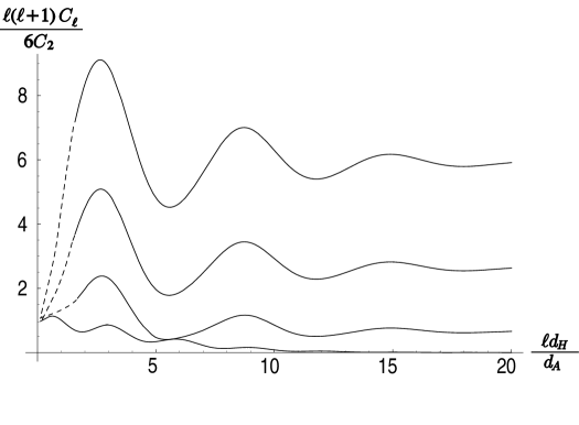
Figure 1: Plots of the ratio of the multipole strength parameter $\ell(\ell+1)C_{\ell}$ to its value at small $\ell$, versus $\ell d_{H}/d_{A}$, where $d_{H}$ is the horizon size at the time of last scattering and $d_{A}$ is the angular diameter distance of the surface of last scattering. The curves are for $\Omega_{B}h^{2}$ ranging (from top to bottom) over the values 0.03, 0.02, 0.01, and 0, corresponding to $\xi$ taking the values 0.81, 0.54, 0.27, and 0. The solid curves are calculated using the WKB approximation; dashed lines indicate an extrapolation to the known value at small $\ell d_{H}/d_{A}$. These results are independent of the parameters $H_{0}$, $\Omega_{\Lambda}$, and $\Omega_{M}$.

For $\Omega_{B}=0$ (in which case the WKB approximation is not needed, so that Eq. (27) should give $C_{\ell}$ down to values of $\ell$ of order two) the behavior of $C_{\ell}$ is nothing like what is observed: $\ell(\ell+1)C_{\ell}/8\pi^{2}B$ rises from unity to 1.1 at a ‘zeroth Doppler peak’ at $\ell d_{H}/d_{A}\simeq 0.45$ (due to the maximum in the Doppler form factor $G(k)$ at $kd_{H}=\pi/2$), then dips to 0.7 at $\ell d_{H}/d_{A}\simeq 1.6$, and then rises again to a first Doppler peak at $\ell d_{H}/d_{A}\simeq 2.83$.

For $\Omega_{B}h^{2}\geq 0.01$ the behavior of $C_{\ell}$ within the range of validity of the WKB approximation is much more like what is observed: $\ell(\ell+1)C_{\ell}$ rises monotonically to a first Doppler peak at $\ell d_{H}/d_{A}$ very roughly of order $\pi$ (though actually around 2.6). There is another clear peak at $\ell\simeq 8.7\,d_{H}/d_{A}$, presumably arising from the peak in $F(k)$ at $k=3\pi/d_{H}$. The weaker peaks in $\ell(\ell+1)C_{\ell}$ arising from peaks in $F(k)$ near even values of $kd_{H}/\pi$ are absent here, presumably because of our neglect of the contribution of radiation and neutrinos to the gravitational field. Another difference between the curves of Figure 1 and more accurate computer calculations is that, again because we neglect the contribution of radiation and neutrinos to the gravitational field, our results do not show the fall-off of $\ell(\ell+1)C_{\ell}$ at large $\ell$ associated with the fall-off of the familiar transfer function $T(k)$ at large $k$.

The values of the position $\ell_{1}d_{H}/d_{A}$ of the first peak and the ratio of its height $\ell_{1}(\ell_{1}+1)C_{\ell_{1}}$ to the value $8\pi^{2}B\simeq 6C_{2}$ for small $\ell$ are given for various baryon densities in Table 1. These results are independent of other parameters. In the last two columns of Table 1 we also give values of $d_{A}/d_{H}$ for $\Omega_{M}=0.3$ and $\Omega_{\Lambda}=0.7$, and the corresponding results for the multipole number $\ell_{1}$ of the first Doppler peak. In calculating the horizon at last scattering $d_{H}$ we have now (somewhat inconsistently) taken into account the effect of photons and three flavors of neutrinos and antineutrinos on the expansion rate, which gives

$$d_{H} \equiv \frac{a(t_{L})}{\sqrt{3}}\int_{0}^{t_{L}}\frac{dt}{a(t)\sqrt{1+R(t)}}$$ (49)

$$= \frac{2}{H_{0}(1+z_{L})^{3/2}\sqrt{3\xi\Omega_{M}}}\ln\left(\frac{\sqrt{1+\xi}+\sqrt{\xi(1+\lambda)}}{1+\sqrt{\xi\lambda}}\right)\;,$$

where $\lambda=0.047/\Omega_{M}h^{2}$ is the ratio of photon and neutrino energy density to dark matter energy density at the time of last scattering, and $d_{A}$ is given by Eq. (2). In calculating the values of $d_{A}/d_{H}$ in the table we have taken $\Omega_{M}h^{2}=0.15$.

Table 1: Location $\ell_{1}d_{A}/d_{H}$ of the first Doppler peak and height of the peak in $\ell(\ell+1)C_{\ell}$ relative to its value $8\pi^{2}B\simeq 6C_{2}$ for $\ell$ extrapolated to zero for various values of the baryon density parameter. These results, and the curves in Figure 1, are independent of the values of $H_{0}$, $\Omega_{\Lambda}$, and (within our approximations) $\Omega_{M}$ and. The last two columns give the values of $d_{A}/d_{H}$ and $\ell_{1}$ for $\Omega_{M}=0.3$, $\Omega_{\Lambda}=0.7$, with $d_{H}$ calculated taking into account the contribution of photons and neutrinos to the expansion rate, and using $\Omega_{M}h^{2}=0.15$.

$\Omega_{B}h^{2}$	$\xi$	$\ell_{1}d_{H}/d_{A}$	$\ell_{1}(\ell_{1}+1)C_{\ell_{1}}/6C_{2}$	$d_{A}/d_{H}$	$\ell_{1}$
0	0	2.83	0.863	91.7	260
0.01	0.27	2.65	2.34	87.1	231
0.02	0.54	2.60	5.09	83.6	217
0.03	0.81	2.58	9.115	79.7	206

We see from Table 1 that the position of the first Doppler peak does not depend strongly on $\Omega_{B}h^{2}$, while its height is a sensitive function of $\Omega_{B}h^{2}$. For $\Omega_{B}h^{2}$ between 0.02 and 0.03 the height and position are in fair agreement with what is observed, though of course the serious comparison of theory with observation relies on more accurate computer calculations. The qualitative results obtained here suggest that if one were to rely on a single feature of the plot of $\ell(\ell+1)C_{\ell}$ versus $\ell$ to measure $\Omega_{B}h^{2}$, then the ratio of the the height of the first Doppler peak to the value for lower $\ell$ values studied by the COBE satellite would be more useful than the ratio of the heights of the first and second Doppler peaks, which relies on less precise data, depends on complicated damping effects, and is more sensitive to other parameters, such as $\Omega_{M}h^{2}$ and the rate of change, if any, of the vacuum energy. Of course, for high precision one must use the whole plot of $\ell(\ell+1)C_{\ell}$ versus $\ell$ to measure all these parameters together.

ACKNOWLEDGMENTS

I am grateful for helpful correspondence with E. Bertschinger, J. R. Bond, L. P. Grishchuk, and M. White. This research was supported in part by the Robert A. Welch Foundation and NSF Grants PHY-0071512 and PHY-9511632.

1. S. Weinberg, ”Fluctuations in the Cosmic Microwave Background I: Form Factors and their Calculation in Synchronous Gauge,” UTTG 03-01, astro-ph/0103279.

2. L. P. Grishchuk and J. Martin, Phys. Rev. D 56, 1924 (1997).

3. J. R. Bond, “Theory and Observations of the Cosmic Background Radiation,” in Cosmology and Large Scale Structure, eds. R. Schaeffer, J. Silk, M. Spiro and J. Zinn-Justin (Elsevier, 1996), Section 5.1.3. Our result (26) can also be derived with somewhat more trouble by using Bond’s results on the asymptotic behavior of averaged products of spherical Bessel functions.

4. This method had been used previously to obtain Eq. (21) with only a scalar form-factor $F(k)$, as for instance by J. R. Bond and G. Efstathiou, Mon. Not. R. Astr. Soc. 226, 655 (1987), Eq. (4.19), but not as far as I know with the inclusion of the dipole form-factor $G(k)$.

5. I. S. Gradshteyn and I. M. Ryzhik, Table of Integrals, Series, and Products (Academic Press, New York, 1980), #6.671.2.

6. I. S. Gradshteyn and I. M. Ryzhik, ibid., #6.574.2.

7. G. ’t Hooft and M. Veltman, Nucl. Phys. B44, 189 (1972).

8. E. F. Bunn and M. White, Ap. J. 480, 6 (1997).