Constraints on diffuse neutrino background from primordial black holes

Abstract

We calculated the energy spectra and the fluxes of electron neutrinos in extragalactic space emitted in the process of the evaporation of primordial black holes (PBHs) in the early universe. It was assumed that PBHs are formed by a blue power-law spectrum of primordial density fluctuations. In the calculations of neutrino spectra the spectral index of density fluctuations and the reheating temperature were used as free parameters. The absorption of neutrinos during propagation in the space was taken into account. We obtained the bounds on the spectral index assuming validity of the standard picture of gravitational collapse and using the available data of several experiments with atmospheric and solar neutrinos. The comparison of our results with the previous constraints (which had been obtained using diffuse photon background data) shows that such bounds are quite sensitive to an assumed form of the initial PBH mass function.

I Introduction

Some recent inflation models (e.g., the hybrid inflationary scenario [1]) predict the ”blue” power-spectrum of primordial density fluctuations. In turn, as is well known, the significant abundance of primordial black holes (PBHs) is possible just in the case when the density fluctuations have an $n>1$ spectrum ($n$ is the spectral index of the initial density fluctuations, $n>1$ spectrum is, by definition, the ”blue perturbation spectrum”).

Particle emission from PBHs due to the evaporation process predicted by Hawking [2] may lead to observable effects. Up to now, PBHs have not been detected, so the observations have set limits on the initial PBH abundance or on characteristics of a spectrum of the primordial density fluctuations. In particular, PBH evaporations contribute to the extragalactic neutrino background. The constraints on an intensity of this background (and, correspondingly, on an PBH abundance) can be obtained from the existing experiments with atmospheric and solar neutrinos. The obtaining of such constraints is a main task of the present paper.

The spectrum and the intensity of the evaporated neutrinos depend heavily on the PBH’s mass. Therefore, the great attention should be paid to the calculation of the initial mass spectrum of PBHs. We use in this paper the following assumptions leading to a prediction of the PBH’s mass spectrum.

1. The formation of PBHs begins only after an inflation phase when the universe returns to the ordinary radiation-dominated era. The reheating process is such that an equation of state of the universe changes almost instantaneously into the radiation type (e.g., due to the parametric resonance [3]) after the inflation.

2. It is assumed, in accordance with analytic calculations [4, 5] that a critical size of the density contrast needed for the PBH formation, $\delta_{c}$, is about $1/3$. Further, it is assumed that all PBHs have mass roughly equal to the horizon mass at a moment of the formation, independently of the perturbation size.

3. Summation over all epochs of the PBH formation can be done using the Press-Schechter formalism [6]. This formalism is widely used in the standard hierarchial model of the structure formation for calculations of the mass distribution functions (see, e.g., [7]).

It was shown recently that near the threshold of a black hole formation the gravitational collapse behaves as a critical phenomenon [8]. In this case the initial mass function will be quite different from that which follows from the standard calculations of refs. [5, 7].The first calculations of the PBH initial mass function (e.g., in ref.[8]) have been done under the assumption that all PBHs form at the same horizon mass (by other words, that all PBHs form at the smallest horizon scale immediately after reheating). The initial PBH mass spectrum for the case of the critical collapse, based on the Press-Schechter formalism, was obtained in the recent work [9].

The calculations in the present paper are based on the standard [4, 5] picture of the gravitational collapse leading to a PBH formation. The case of the critical collapse will be considered in a separate work.

The plan of the paper is as follows.

In Sec.II we give, for completeness, the brief derivation of a general formula for the initial PBH mass spectrum. The final expression is presented in a form, which is valid for an arbitrary relation between three physical values: the initial PBH mass, the fluctuation mass (i.e., the mass of the perturbed region) at a moment of the collapse, and the density contrast in the perturbed region (also at a moment of the collapse). This expression contains the corresponding results obtained in refs. [7, 9] as particular cases. As in refs. [7, 9], the derivation is based on the linear perturbation theory and on the assumption that a power spectrum of the primordial fluctuations can be described by a power law.

In Sec.III we derive the approximate formula for a calculation of the extragalactic neutrino background from PBH evaporations. We do not use cosmological models of the inflation and of the spectrum of primordial fluctuations, so there are two free parameters: the reheating temperature and the spectral index. At the end of the section, some examples of instantaneous neutrino spectra from the evaporation of an individual black hole are presented.

In Sec.IV we perform the normalization of the primordial power spectrum of density perturbations by COBE data on the angular power spectrum of CMB temperature fluctuations. We consider the case of flat cosmological models with nonzero cosmological constant. We show, that the result of this normalization rather weakly depends on the matter content of the present Universe, $\Omega_{m}=1-\Omega_{\Lambda}$.

In Sec.V we present the results of numerical calculations of the neutrino background spectra from PBH evaporations, with taking into account the effects of neutrino absorption in the space. For background neutrino energies $\sim 10-100\;MeV$ we studied relative contributions to the background intensity of different cosmological redshifts (and it is shown that at high reheating temperatures the characteristic values of the redshifts are very large).

In Sec.VI we consider the possibilities of constraining the spectral index, using experiments with neutrinos of natural origin.

In Sec.VII the spectral index constraints, followed from our calculations and from available data of the neutrino experiments, are given.

II The initial mass spectrum of PBHs

As is pointed out in the Introduction, we use the Press-Schechter formalism which allows to carry out the summation over all epochs of PBHs formation. According to this formalism, the mass spectrum of density fluctuations ( i.e., the number density of regions with mass between $M$ and $M+dM$ ) is calculated by the formula

$$n\left(M,\delta_{c}\right)dM=\frac{\rho_{i}}{M}\left|\frac{\partial\beta}{\partial M}(M,\delta_{c})\right|dM\;\;\;.$$ (1)

Here, $\beta(M,\delta_{c})$ is the fraction of regions having sizes larger than $R$ and density contrast larger than $\delta_{c}$ ,

$$\beta(M,\delta_{c})=2\int^{\infty}_{\delta_{c}}P(M,\delta)d\delta\;\;\;,$$ (2)

$$P(M,\delta)=\frac{1}{\sqrt{2\pi}\sigma_{R}(M)}\exp\left(-\frac{\delta^{2}}{2\sigma_{R}^{2}(M)}\right)\;\;\;.$$ (3)

In these formulas, $\delta$ is the initial density contrast, $\sigma_{R}$ is the standard deviation of the density contrast of the regions with a comoving size $R$ and mass $M$. The factor of $2$ in Eq.(2) ensures the correct normalization of $n(M,\delta_{c})$, integrated over all $M$. This factor is usually added to take into account (approximately) the contribution of underdense regions to gravitationally bound objects [7].

It is convenient to introduce the double differential distribution $n(M,\delta)$, the integral over which gives the total number of fluctuated regions:

$$n=\int\!\!\!\!\int n(M,\delta)dMd\delta\;\;\;\;,\;\;\;n(M,\delta_{c})=\int n(M,\delta)d\delta\;\;\;.$$ (4)

Using Eqs.(1-3), for $n(M,\delta)$ one has the expression

$$n(M,\delta)=\sqrt{\frac{2}{\pi}}\frac{\rho_{i}}{M}\frac{1}{\sigma_{R}^{2}(M)}\frac{\partial\sigma_{R}}{\partial M}\left|\left(\frac{\delta^{2}}{\sigma_{R}^{2}(M)}-1\right)\right|\exp\left(-\frac{\delta^{2}}{2\sigma_{R}^{2}(M)}\right)\;\;\;.$$ (5)

To obtain the mass spectrum of PBHs one must introduce the $M_{BH}$ variable. Besides, we will use the variable $\delta^{\prime}$, connected with $\delta$ by the relation

$$\delta^{\prime}=\delta\left(\frac{M}{M_{i}}\right)^{2/3}\;\;.$$ (6)

Here, $M_{i}$ is the horizon mass at the moment of a beginning of the growth of density fluctuations. This new variable is the density contrast at the moment of the collapse. The new distribution function is

$$n_{BH}(M_{BH},\delta^{\prime})=n(M_{BH},\delta)\frac{d\delta}{d\delta^{\prime}}\frac{dM}{dM_{BH}}\;\;.$$ (7)

Further, we assume that there is some functional connection between $M_{BH}$, $M$ and $\delta^{\prime}$:

$$M_{BH}=f(M,\delta^{\prime})\;\;.$$ (8)

In this case one can rewrite Eq.(7) in the form

$$n_{BH}(M_{BH},\delta^{\prime})=n\left(M,\delta^{\prime}\left(\frac{M}{M_{i}}\right)^{-2/3}\right)\cdot\left(\frac{M}{M_{i}}\right)^{-2/3}\cdot\frac{1}{{df(M,\delta^{\prime})}/{dM}}$$ (9)

and the PBH mass spectrum is given by the integral

$$n_{BH}(M_{BH})=\int n_{BH}(M_{BH},\delta^{\prime})d\delta^{\prime}\;.$$ (10)

Now, to connect the mass spectrum with the spectral index one can use the relations

$$\sigma_{R}=\sigma_{H}(M)\left(\frac{M}{M_{i}}\right)^{-2/3}\;\;,\;\;\sigma_{H}(M)\sim M^{\frac{1-n}{6}}.$$ (11)

In these relations $\sigma_{H}(M)$ is the horizon crossing amplitude, i.e., the standard deviation of the density contrast in the perturbed region at the moment when this fluctuation crosses horizon. The derivation of Eqs.(11) is given, for completeness, in Sec.IV.

Using Eqs.(11) in the expression (5) for $n(M,\delta)$ one obtains

$$n(M,\delta)=-\frac{n+3}{6}\cdot\sqrt{\frac{2}{\pi}}\frac{\rho_{i}}{M_{i}^{2}}\frac{1}{\sigma_{H}}\left(\frac{M}{M_{i}}\right)^{-4/3}\left|\frac{\delta^{2}}{\sigma_{R}^{2}}-1\right|e^{-{\delta^{2}}/{2\sigma_{R}^{2}}}\;\;.$$ (12)

Substituting this expression in the r.h.s. of the Eq.(9) and using Eq(10) one has

$$n_{BH}(M_{BH})=\frac{n+3}{6}\cdot\sqrt{\frac{2}{\pi}}\rho_{i}\int\frac{1}{M^{2}\sigma_{H}}\left|\frac{{\delta^{\prime}}^{2}}{\sigma_{H}^{2}}-1\right|e^{-\frac{{\delta^{\prime}}^{2}}{2\sigma_{H}^{2}}}\frac{1}{df(M,\delta^{\prime})/dM}d{\delta^{\prime}}\;\;.$$ (13)

Values of $M$ in r.h.s of Eq.(13) are expressed through $M_{BH}$, $\delta^{\prime}$ by the relation (8).

Formula (13) is the final expression for the PBH mass spectrum, the main result of this Section. It is valid for any relation between PBH mass $M_{BH}$, mass of the original overdense region $M$ and the density contrast $\delta^{\prime}$.

In the particular case of a near critical collapse

$$f(M,\delta^{\prime})=M_{i}^{1/3}M^{2/3}k(\delta^{\prime}-\delta_{c})^{\gamma_{k}}\equiv\xi M^{1/3}_{i}M^{2/3}\;,$$ (14)

therefore

$$M=M_{BH}^{3/2}M_{i}^{-1/2}\xi^{-3/2}\;\;;\;\;df/dM=\frac{2}{3}M_{i}^{1/2}M_{BH}^{-1/2}\xi^{3/2}\;\;.$$ (15)

Eq.(14) can be rewritten in the form, derived in the ref. [8], using the connection between $M$ and the horizon mass $M_{h}$ (which is equal to a fluctuation mass at the moment when the fluctuation crosses horizon):

$$M_{h}=M_{i}^{1/3}M^{2/3}\;\;.$$ (16)

The resulting formula for the spectrum,

$$n_{BH}(M_{BH})=\frac{n+3}{4}\sqrt{\frac{2}{\pi}}\rho_{i}\sqrt{M_{i}}M_{BH}^{-5/2}\int^{1}_{\delta_{c}}\frac{1}{\sigma_{H}}\left|\frac{\delta^{\prime}{}^{2}}{\sigma_{H}^{2}}-1\right|e^{-\frac{\delta^{2}}{2\sigma_{H}^{2}}}\xi^{3/2}d\delta^{\prime}\;\;,$$ (17)

coincides, as can be easily proved, with the expression derived in ref. [9].

The mass spectrum formula for the Carr-Hawking collapse can be obtained analogously, with the relation $f(M,\delta^{\prime})=\gamma^{1/2}M_{i}^{1/3}M^{2/3}$ (see Eq.(32) below), or from Eq.(17) using the substitutions

$$\gamma_{k}\to 0\;\;,\;\;k\to\gamma^{1/2}\;\;,\;\;\delta_{c}\to\gamma$$ (18)

and the approximate relation

$$\int^{1}_{\gamma}d\delta^{\prime}\left(\frac{\delta^{\prime}{}^{2}}{\sigma_{H}^{2}}-1\right)e^{-\frac{\delta^{\prime}{}^{2}}{2\sigma_{H}^{2}}}\approx\gamma e^{-\frac{\gamma^{2}}{2\sigma_{H}^{2}}}\;\;.$$ (19)

In this case one obtains the expression derived in ref. [7]:

$$n_{BH}(M_{BH})=\frac{n+3}{4}\sqrt{\frac{2}{\pi}}\gamma^{7/4}\rho_{i}M_{i}^{1/2}M_{BH}^{-5/2}\sigma_{H}^{-1}\exp\left(-\frac{\gamma^{2}}{2\sigma_{H}^{2}}\right)\;.$$ (20)

One can see from Eqs.(17) and (20) that the PBH mass spectrum following from the Press-Shechter formalism has quasi power form in both considered cases $\left(\sim M_{BH}^{-5/2}\right)$. In Carr-Hawking case $M_{BH}^{min}\sim M_{h}$ , in contrast with this in the critical collapse case it is possible that $M_{BH}\ll M_{h}$ .

III Formula for neutrino diffuse background from PBHs

The starting formula for a calculation of the cosmological background from PBH evaporations is [10]

$$S(E)=\int n_{com}\frac{1}{4\pi a_{0}^{2}\rho^{2}_{\mathstrut}}f\left(E(1+z)\right)dV_{com}\;\;\;.$$ (21)

Here , $n_{com}$ is the comoving number density of the sources (in our case the source is an evaporating PBH of the definite mass $m$ ), $a_{0}$ is the scale factor at present time, $t=t_{0}$, $f(E)$ is a differential energy spectrum of the source radiation. $V_{com}$ is a comoving volume of the space filled by sources, therefore

$$dV_{com}=a_{0}^{3}\frac{\rho^{2}d\rho}{\sqrt{1-k\rho^{2}}}d\Omega\;\;\;.$$ (22)

Here, $k$ is the curvature coefficient, and $\rho$ is the radial comoving coordinate. Using the change of the variable,

$$\frac{d\rho}{\sqrt{1-k\rho^{2}}}=\frac{dt}{a}\;\;\;,$$ (23)

the comoving number density can be expressed via the initial density $n_{i}$,

$$n_{com}=n_{phys}(t_{0})=n_{i}\left(\frac{a_{i}}{a}\right)^{3}\left(\frac{a}{a_{0}}\right)^{3}=n_{i}\left(\frac{a_{i}}{a_{0}}\right)^{3}\;\;\;\;.$$ (24)

Substituting Eqs. (22) - (24) in Eq. (21) one obtains

$$S(E)=n_{i}\int dt\frac{a_{0}}{a}\left(\frac{a_{i}}{a_{0}}\right)^{3}f\left(E(1+z)\right)\;\;\;.$$ (25)

In our concrete case the source of the radiation is a Hawking evaporation:

$$n_{i}f\left(E(1+z)\right)=\int dm\,n_{BH}(m,t)f_{H}\left(E(1+z),m\right)\;\;\;.$$ (26)

Here , $n_{BH}(m,t)$ is the PBH mass spectrum at any moment of time, $f_{H}(E,m)$ is the Hawking function [2],

$$f_{H}\left(E,m\right)=\frac{1}{2\pi\hbar}\frac{\Gamma_{s}(E,m)}{exp\left(\frac{8\pi GEm}{\hbar c^{3}}\right)-(-1)^{2s}}\;\;\;.$$ (27)

Here, $E$ is the energy of an evaporated particle (it lies in the interval [$0$,$\infty$] for massless particles), $\Gamma_{s}(E,m)$ is the coefficient of the absorption by a black hole of a mass $m$, for an particle having spin s and energy $E$.

In our calculations (we considered only the simplest case of a nonrotating uncharged hole) we used the approximation when $\Gamma_{s}$ depends only on $mE$ (as is the case for massless particles), i.e. we ignore the decrease of $\Gamma_{s}$ at nonrelativistic energies of evaporated particles. But, working in this massless limit, we nevertheless used in a low $mE$ region the exact forms of $\Gamma_{s}$, which are obtained numerically (concretely, we used the plots for absorption cross section, $\sigma\approx\Gamma_{s}/{E^{2}}$, as a function of $mE$, for $s=1/2$ and $s=1$, from the Fig.1 of work [11]), rather than the low-energy limits obtained analytically in works [12, 13].

The initial spectrum of PBHs is given by Eq. (20). The minimum value of PBH mass in the specrtum can be obtained from the following considerations. It is known [5] that the condition of a recollapse of the perturbed region is the following: radius of a maximum expansion of this region, $R_{c}$, must obey the inequality

$$R_{c}>\gamma^{1/2}R_{h}=\gamma^{1/2}(ct_{c})\;.$$ (28)

Here, $R_{h}$ is the horizon radius at $t_{c}$, the moment of time, when the radius of the perturbation region is equal to maximum one. It is known also [5] that $t_{c}$ and $t_{i}$, the initial moment of time, are connected by the relation

$$\frac{t_{i}}{t_{c}}\sim\delta_{i}\;,$$ (29)

where $\delta_{i}$ is the initial density contrast for which there is the condition following from Eq.(28):

$$\delta_{i}\gtrsim\gamma\left(\frac{M}{M_{i}}\right)^{-2/3}.$$ (30)

Using Eq.(28) and the formula for horizon mass at $t_{i}$,

$$M_{i}=\frac{4}{3}\pi(ct_{i})^{3}\rho(t_{i})\;\;,$$ (31)

one obtains the connection between $M_{BH}$ and $t_{c}$:

$$M_{BH}=\frac{4}{3}\pi R_{c}^{3}\rho(t_{c})=\gamma^{3/2}M_{i}\frac{t_{c}}{t_{i}}\;.$$ (32)

The use of Eqs.(29,30) in Eq.(32) leads to the relation [7]

$$M_{BH}=\gamma^{1/2}M_{i}^{1/3}M^{2/3}\;.$$ (33)

From Eq.(33) one follows that the minimum value of a PBH mass in the PBH mass spectrum is given by the simple formula

$$M_{BH}^{min}=\gamma^{1/2}M_{i}\;.$$ (34)

Strictly speaking, the minimum value of $\frac{t_{c}}{t_{i}}$ is equal to $1$ (corresponding to $\delta_{i}^{max}=1$). Therefore, the absolute minimum value of PBH mass, following from Eq.(32), is equal to $\gamma^{3/2}M_{i}$. However, the use of such a value as a border value of the PBH mass spectrum is clearly inconsistent. It contradicts with the relation (33) and, in general, with the fact that, due to the exponential damping [7], the bulk of the PBH intensity is determined just by the minimum value of $\delta_{i}$ (given by Eq.(30)).

To take into account the existence of the minimum we must add to the initial spectrum expression the step factor $\Theta(M_{BH}-\gamma^{1/2}M_{i})$. The connection of the initial mass value $M_{BH}$ and the value at any moment $t$ is determined by the solution of the equation [12]

$$\frac{dm}{dt}=-\frac{\alpha(m)}{m^{2}}\;\;.$$ (35)

The function $\alpha(m)$ accounts for the degrees of freedom of evaporated particles and determines the lifetime of a black hole. In the approximation $\alpha=const$ the solution of Eq.(35) is

$$M_{BH}\cong\left(3\alpha t+m^{3}\right)^{1/3}\;\;\;.$$ (36)

This decrease of PBH mass leads to the corresponding evolution of a form of the PBH mass spectrum. At any moment one has

$$n_{BH}(m,t)dm=\frac{m^{2}}{\left(3\alpha t+m^{3}\right)^{2/3}}n_{BH}\left((3\alpha t+m^{3})^{1/3}\right)\times\Theta\left[m-\left((\gamma^{1/2}M_{i})^{3}-3\alpha t\right)^{1/3}\right]dm.$$ (37)

Substituting Eqs. (27), (37) in the integral in Eq.(26) , we obtain the final expression for the spectrum of the background radiation:

$$S(E)=\frac{c}{4\pi}\int dt\frac{a_{0}}{a}\left(\frac{a_{i}}{a_{0}}\right)^{3}\int dm\frac{m^{2}}{(3\alpha t+m^{3})^{2/3}}n_{BH}\left[\left(3\alpha t+m^{3}\right)^{1/3}\right]\times$$ (38)

(39)

$$\Theta\left[(m-\left((\gamma^{1/2}M_{i})^{3}-3\alpha t\right)^{1/3}\right]g_{\nu}f_{H}(E(1+z),m)\;\;\;.$$ (40)

Here, $g_{\nu}$ is a number of degrees of freedom. In the following we will interest in ($\nu_{e}+\tilde{\nu}_{e}$) - spectrum, so $g_{\nu}=2$.

One should note that the corresponding expressions for the spectrum in refs. [14, 15] contain the factor $\left(\frac{a_{i}}{a}\right)^{3}$ instead of the correct factor $\left(\frac{a_{i}}{a_{0}}\right)^{3}$. It leads to a strong overestimation of large $z$ contributions in $S(E)$ (see below, Fig.5).

It is convenient to use in Eq.(38) the variable $z$ instead of $t$. In the case of flat models with nonzero cosmological constant one has

$$\frac{dt}{dz}=-\frac{1}{H_{0}(1+z)}\left(\Omega_{m}(1+z)^{3}+\Omega_{r}(1+z)^{4}+\Omega_{\Lambda}\right)^{-1/2}\;\;\;,$$ (41)

$$\Omega_{r}=(2.4\cdot 10^{4}h^{2})^{-1}\;\;\;\;,\;\;\;\Omega_{m}=1-\Omega_{r}-\Omega_{\Lambda}\;\;\;.$$ (42)

The factor $(\frac{a_{i}}{a_{0}})^{3}$ can be expressed through the value of $t_{eq}$, the moment of matter-radiation density equality:

$$\left(\frac{a_{i}}{a_{0}}\right)^{3}\simeq(1+z_{eq})^{-3}\left(\frac{t_{i}}{t_{eq}}\right)^{3/2}=\left(\frac{2}{3}(2-\sqrt{2})\right)^{-3/2}H_{0}^{3/2}\left(2.4\cdot 10^{4}h^{2}\right)^{-3/4}t_{i}^{3/2}\;\;\;.$$ (43)

The constant $H_{0}$, entering the Eqs.(41,43) is connected with $h$ by definition:

$$H_{0}=100h\text{ km}\text{ s}^{-1}\text{ Mpc}^{-1}\;.$$ (44)

Throughout the paper we suppose that $h=0.67$. One can see from Eqs.(43,44) that the factor $\left(\frac{a_{i}}{a_{0}}\right)^{3}$ does not depend on $h$ and $\Omega_{m}$, as it must be.

Integrating over PBH’s mass in Eq.(38), one obtains finally, after the change of the variable $t$ on $z$, the integral over $z$:

$$S(E)=\int\,F(E,z)d\log_{10}(z+1)\;\;\;.$$ (45)

In analogous calculations of the photon diffuse background integral over $z$ in the expression for $S(E)$ is cut off at $z=z_{0}\approx 700$ because for larger $z$ the photon optical depth will be larger than unity [16]. In contrast with this , interactions of neutrinos with the matter can be neglected up to very high values of $z$. Therefore the neutrino diffuse background from PBH evaporations is much more abundant. The neutrino absorption effects are estimated below, in Sec.VI.

The evaporation process of a black hole with not too small initial mass is almost an explosion. So, for a calculation of spectra of evaporated particles with acceptable accuracy it is enough to know the value of $\alpha$ for an initial value of the PBH mass only. Taking this into account and having in mind the steepness of the PBH mass spectrum, we use the approximation

$$\alpha(m)=\alpha(M_{BH}^{min})=\alpha(\gamma^{1/2}M_{i})\;\;,$$ (46)

and just this value of $\alpha$ is meant in the expressions (36)-(38).

The very detailed calculation of the function $\alpha(m)$ was carried out in the works [11, 17]. Here we use the simplified approach in which $\alpha(m)$ is represented by the dependence

$$\alpha=\alpha_{0}+\sum\limits_{i}a_{i}\cdot 10^{25}\cdot\Theta(b_{i}-log_{10}(m)).$$ (47)

TABLE I.: Coefficients $a_{i}$ and $b_{i}$ in Eq.(47)

$i$	$\mu$	u,d	g	s	$\tau$	c	b	$W^{\pm}$	$Z^{0}$	t
$a_{i}$	3.12	9.36	4.96	9.36	3.12	9.36	9.36	1.86	0.93	9.36
$b_{i}$	14.59	14.13	13.97	13.89	13.35	13.32	12.91	11.87	11.85	11.39

Here, $\Theta(x)$ is the step function. Coefficient $\alpha_{0}$ gives the summary contribution of $e^{+}$, $e^{-}$, $\nu$ and $\gamma$ and is equal to $8.42\cdot 10^{25}\;g^{3}sec^{-1}$ [12, 17]. All other coefficients are collected in the Table I.

The coefficients $b_{i}$ determine the value of the PBH mass beginning from which particles of $i$-type can be evaporated. This value, $M_{BH}^{b_{i}}$, is obtained from the relations

$$\left(\frac{10^{13}g}{M_{BH}^{b_{i}}}\right)\text{ GeV}\cong kT_{BH}^{b_{i}}\cong\frac{m_{i}}{\kappa(s_{i})}\;,$$ (48)

$$\kappa(\frac{1}{2})\approx 4\;\;\;,\kappa(1)\approx 6\;.$$ (49)

So,

$$b_{i}=log_{10}M_{BH}^{b_{i}}\;\;.$$ (50)

Writing Eqs.(48,49) we took into account that the evaporation of massive particles becomes essential once the peak value in the energy distribution exceeds the particle rest mass. The peak value depends on the particle spin (see, e.g., [11]):

$$E_{peak}(s=1/2)\approx 4kT_{BH}\;\;\;;\;\;\;E_{peak}(s=1)\approx 6kT_{BH}\;.$$ (51)

The values of masses of (u,d,s,c,b,g,$\tau$)-particles used in our calculations of $b_{i}$ are the same as in work [17], top quark mass was taken equal to $170\text{GeV}$. The resulting function $\alpha(m)$ is shown on Fig.1. For comparison, the corresponding dependence from the work [17] (drawn using the Eq.7 of [17]) is also shown.

According to Eq.(34) the minimum value of PBH mass in the mass spectrum is about the horizon mass $M_{i}$. In turn, the value of $M_{i}$ is connected with $t_{i}$, the moment of time just after reheating, from which the ”normal” radiation era and the process of PBHs formation start,

$$M_{i}=\frac{1}{8}\frac{M_{pl}}{t_{pl}}t_{i}\;.$$ (52)

The corresponding reheating temperature is given, approximately, by the relation (see Eq.(113))

$$kT_{RH}\simeq\left(\frac{t_{i}}{1s}\right)^{-1/2}\text{MeV}\;.$$ (53)

If $kT_{RH}$ values lie in the interval $(10^{8}-10^{10})\text{ GeV}$ (just for this interval we obtain the spectral index constraints in the present paper), the corresponding $M_{i}$ values lie in the mass interval $(10^{11}-10^{15})\text{ g}$. So, as one can see, we really need for our aims the all information about $\alpha$-parameter, that contains in Fig.1, including the highest values of $\alpha$ at $m\sim 10^{11}\text{ g}$.

The formula (38), as it stands, takes into account the contribution to the neutrino background solely from a direct process of the neutrino evaporation. If we suppose that particles evaporated by a black hole propagate freely, the calculation of other contributions to the neutrino background can be performed using our knowledge of particle physics [11, 17].

On Fig.2 the typical result of our calculation of instantaneous neutrino spectra from evaporating black hole is shown. The spectrum of the straightforward (direct) $(\nu_{e}+\tilde{\nu}_{e})$ - emission is given by the Hawking function $f_{H}(E,m)$, Eq.(27). The $(\nu_{e}+\tilde{\nu}_{e})$ spectrum arising from decays of $(\mu^{+}+\mu^{-})$ evaporated directly is calculated by the formula

$$f^{(\mu)}(E,m)=\int\Theta(b_{\mu}-\log_{10}m)g_{\mu}f_{H}(E_{\mu},m)\frac{dn_{\nu}(E_{\mu},E)}{dE}dE_{\mu}\;\;,$$ (54)

where $dn^{\mu}_{\nu}/dE$ is the neutrino spectrum in a $\mu$ - decay, $g_{\mu}=4$. To evaluate the electron neutrino spectrum resulted from fragmentations of evaporated quarks, we used the simplest chain

$$(u,d)-\mbox{quarks}\;\;\longrightarrow\;\;\pi\;\;\longrightarrow\;\;\mu\;\;\longrightarrow\;\;\nu_{e}\;\;,$$ (55)

and the formula

$$f^{(q)}(E,m)=\int\Theta(b_{q}-\log_{10}m)g_{q}f_{H}(E_{q},m)\frac{dn^{q}_{\pi}(\xi)}{d\xi}\cdot\frac{d\xi}{dE_{q}}\cdot\frac{dn_{\mu}^{\pi}(E_{\mu},E_{\pi})}{dE_{\mu}}\cdot\frac{dn^{\mu}_{\nu}(E_{\mu},E)}{dE}dE_{q}dE_{\pi}dE_{\mu}\;\;.$$ (56)

Here, $g_{q}=24$ for a summary contribution from $u,\;\tilde{u},\;d,\;\tilde{d}$ - quarks, ${dn^{q}_{\pi}}/{d\xi}$ is the $q\to\pi$ fragmentation function, for which the simple parametrization was taken:

$$\frac{dn^{q}_{\pi}}{d\xi}=\frac{15}{16}(\xi-1)^{2}\xi^{-3/2}\;\;,\;\;\xi=\frac{E_{\pi}}{E_{q}}\;\;,$$ (57)

and ${dn_{\mu}^{\pi}}/{dE_{\mu}}$ is the $\mu$ - spectrum in a decay $\pi\to\mu+\nu_{\mu}$.

Analogous formulas are used for calculations of the neutrino spectrum from other channels of the neutrino production, for instance from decays of evaporated $W$-bosons ($W\to e+\nu_{e}\;\;,$ $W\to\mu\to\nu_{e}$).

The formula (57) for the fragmentation function was suggested in the paper [18]. It leads to a simple multiplicity growth law of $\sqrt{E}$ (such a law follows from a naive statistical model of an jet fragmentation ). It had been shown in ref. [18] that Eq.(57) fits rather well the PETRA data and can be used instead of the more ingenious formula based on the leading logarithm approximation of QCD. In turn, it was shown recently [19] using the programme HERWIG [20] that the parametrizations of ref. [18], being rather good at low $\xi$, lead to an significant overestimation of the yield of large $\xi$ final states. This fact as well as the simplicity of Eq.(57) were decisive for our choice of the fragmentation function because, as we will show, we need just the upper estimate of the yield of quark fragmentations.

In all calculations in the present paper we neglected the contribution to neutrino fluxes from neutron decays in the jets. These decays give the distinct bumps in instantaneous $\nu\tilde{\nu}$-spectra at $E\sim 1\mbox{ MeV}$ [11]. In general, neutrinos of such low energies have too small cross sections for neutrino-nucleus and neutrino-nucleon interactions (see sec.VI) and are inessential for our main aim: the constraining of the spectral index (neutrinos with energies $\sim 10-100\mbox{ MeV}$ are mainly responsible for this). Besides, we will see at Sec.V that at large values of one of the parameters of our approach (reheating temperature $T_{RH}$) these neutrinos are not noticeable in the summary neutrino background even at $E\sim 1\mbox{ MeV}$ because of strong redshift effects.

In order to check the accuracy of our calculations of instantaneous neutrino spectra we calculated for one value of a black hole temperature the summary neutrino spectrum (excluding secondary $\nu_{\tau}$ only). The result is shown on Fig.3 together with the corresponding curve from ref.[11]. One can see from this figure that in the practically interesting region of neutrino energies ($E>100\text{ MeV}$) our result differs from the Monte-Carlo result of ref.[11] not more than on a factor of 2.

The relative contribution of different channels to the total $\nu_{e}$ spectrum strongly depends on the black hole temperature. One can see from Fig.2, that at high temperature decays of massive particles evaporated by the black hole become rather important at high energy tail of the spectrum (if the corresponding branching ratios are not too small).

The total instantaneous neutrino spectrum from a black hole evaporation is given by the sum

$$f(E,m)=g_{\nu}f_{H}(E,m)+f^{(\mu)}(E,m)+f^{(q)}(E,m)+...\;\;\;,$$ (58)

and the total background neutrino spectrum is given by the same Eq.(38), except the change $g_{\nu}f_{H}(E,m)\to f(E,m)$.

IV Normalization of the perturbation amplitude

For numerical calculations of the neutrino background we need normalization of the dispersion $\sigma_{R}$ entering the PBH mass spectrum formula. For this aim we must consider the time evolution of this dispersion. The connection of $\sigma_{R}(t)$ with a power spectrum $P(k,t)$ of the density perturbations is given by the expression

$$\sigma_{R}^{2}(t)=\int\limits_{0}^{\infty}\frac{k^{3}}{2\pi^{2}}P(k,t)W^{2}(kR)\frac{dk}{k}\equiv$$ (59)

(60)

$$\int\limits_{0}^{\infty}\frac{k^{4}}{(aH)^{4}}\delta_{H}^{2}(k,t)W^{2}(kR)\frac{dk}{k}\;.$$ (61)

Here, $W(kR)$ is the smoothing window function. The second line of this equation defines the (nonsmoothed) horizon crossing amplitude $\delta_{H}(k,t)$. In general, it depends on the time and we need the initial amplitude $\delta_{H}(k,t_{i})$, whereas the normalization on COBE data (which had been performed, in particular, in the work [21]) determines this amplitude at present time, $t=t_{0}$. Only in the particular case of a flat cosmological model with $\Lambda=0$ the horizon crossing amplitude is time-independent and the normalization on COBE data gives $\delta_{H}(k,t_{i})$ straightforwardly.

Assuming a power law of primordial density perturbations,

$$P(k,t)\sim k^{n},$$ (62)

and choosing for $W(kR)$ the top-hat form,

$$W(kR)=\frac{3j_{1}(kR)}{kR},$$ (63)

one obtains from Eq.(59)

$$\sigma_{R}^{2}(t)=C_{n}^{2}\frac{k_{fl}^{4}}{(aH)^{4}}\delta_{H}^{2}(k_{fl},t)\equiv\frac{k_{fl}^{4}}{(aH)^{4}}\sigma_{H}^{2}(k_{fl},t)\;.$$ (64)

In Eq.(64), $k_{fl}$ is the comoving wave number, characterizing the perturbed region,

$$k_{fl}=\frac{1}{R}$$ (65)

and $C_{n}$ is a constant which depends on the spectral index $n$. For $n\simeq 1$ one has $C_{n}\simeq 4.8$ . The fluctuation power per logarithmic interval, or variance, at present time is given by the expression [22]

$$\frac{k^{3}}{2\pi^{2}}P(k,t_{0})=\frac{1}{H_{0}^{4}}k^{4}A_{S}^{2}(k)\frac{g^{2}(\Omega_{m})}{\Omega_{m}^{2}}\;.$$ (66)

Here, $A_{S}(k)$ is an amplitude of the scalar perturbations, k-dependence of which arises from a deviation from scale invariance ($A_{S}^{2}\sim k^{n-1}$). The factor $g^{2}(\Omega_{m})$ takes into account the suppression of the growth of density perturbations due to nonzero $\Omega_{\Lambda}$ (density perturbations stop growing once the universe becomes cosmological constant dominated). The factor $\Omega_{m}^{2}$ in the denominator of Eq.(66) arises because the potential fluctuations are reduced by $\Omega_{m}$: due to this, for fixed COBE normalization, the power spectrum of density perturbations must be, aside from other factors, enhanced by $\Omega_{m}^{-2}$ [23].

For arbitrary moment of time in matter era the expression for the power spectrum is evident generalization of Eq.(66):

$$\frac{k^{3}}{2\pi^{2}}P(k,t)=\frac{k^{4}}{H_{0}^{4}}A_{S}^{2}(k)\left(\frac{g(a,\Omega_{m})}{\Omega_{m}}\right)^{2}\;.$$ (67)

Here, the function $g(a,\Omega_{m})$ accounting for the growth of density perturbations is given by the expression [24]

$$g(a,\Omega_{m})=\frac{5\Omega_{m}}{2a}\frac{da}{d\tau}\int\limits_{0}^{a}\left(\frac{da^{\prime}}{d\tau}\right)^{-3}da^{\prime},$$ (68)

where $\tau\equiv H_{0}t$. In our case

$$\frac{da}{d\tau}=\Omega_{m}\cdot\frac{1}{a}+\Omega_{\Lambda}a^{2}$$ (69)

and

$$g(a,\Omega_{m})=\frac{5}{2}\Omega_{m}a^{-3/2}(\Omega_{m}+\Omega_{\Lambda}a^{3})^{1/2}\int\limits^{a}_{0}\frac{x^{3/2}dx}{(\Omega_{m}+\Omega_{\Lambda}x^{3})^{3/2}}\;.$$ (70)

The normalization of this function is such that

$$g(a,1)=a\;.$$ (71)

For the present time ($a=a_{0}=1$) one has

$$g(1,\Omega_{m})=g(\Omega_{m})\;,$$ (72)

where $g(\Omega_{m})$ is the function entering Eq.(66), as it must be. The horizon crossing amplitude $\delta_{H}(k,t)$ defined by the Eq.(59) is determined by the relation

$$\delta_{H}^{2}(k,t)=\frac{(aH)^{4}}{H_{0}^{4}}A_{S}^{2}(k)\left(\frac{g(a,\Omega_{m})}{\Omega_{m}}\right)^{2}\;\stackrel{{\scriptstyle t\to t_{0}}}{{\longrightarrow}}\;A_{S}^{2}(k)\left(\frac{g(\Omega_{m})}{\Omega_{m}}\right)^{2}\;.$$ (73)

One can see that the time dependence of $\delta_{H}(k,t)$ arises just due to nonzero value of $\Lambda$. If $\Lambda=0$, one has from Eq.(73), using Eq.(71),

$$\left.\delta_{H}^{2}(k,t)\right|_{\Lambda=0}=A_{S}^{2}(k)\;.$$ (74)

Our normalization of perturbation amplitude on COBE data is based on two inputs.

1. Connection between CMB fluctuations and scalar density fluctuations is described [22] by the following relations (derived for a lowest-order reconstruction of the inflationary potential):

$$S\equiv\frac{5C^{2}_{S}}{4\pi}=0.104f_{S}^{(0)}(\Omega_{\Lambda})A_{S}^{2}(k_{*})\;,$$ (75)

$$f_{S}^{(0)}(\Omega_{\Lambda})=1.04-0.82\Omega_{\Lambda}+2\Omega_{\Lambda}^{2}\;,$$ (76)

$$0.0\leq\Omega_{\Lambda}\leq 0.8\;.$$ (77)

Here, $C^{S}_{2}$ is the scalar contribution to the angular power spectrum of CMB temperature fluctuations for $l=2$, $k_{*}\sim a_{0}H_{0}$ is the comoving wave number at the present horizon scale. The dependence $f_{S}^{(0)}$ on $\Omega_{\Lambda}$ is due to the integrated Sachs-Wolfe effect, i.e., due to the evolution of the potentials from last scattering surface till the present time.

2. From 4-year COBE data [25] one has (assuming that the scalar contribution dominates over the tensor on the large scales) the following results for small $l$ values [26]:

$$\left(\frac{l(l+1)C_{l}^{S}}{2\pi}\right)^{1/2}\simeq(1.03\pm 0.07)\cdot 10^{-5},$$ (78)

$$n=1.02\pm 0.24\;.$$ (79)

From Eqs.(73-78) one obtains, finally, the normalization of the horizon crossing amplitude:

$$\delta_{H}(k_{*},t_{0})\equiv\delta_{H}^{(COBE)}\simeq 2\cdot 10^{-5}\frac{1}{\sqrt{f^{(0)}_{S}(\Omega_{\Lambda})}}\left(\frac{g(\Omega_{m})}{\Omega_{m}}\right),$$ (80)

$$A_{S}(k_{*})=2\cdot 10^{-5}\frac{1}{\sqrt{f^{(0)}_{S}(\Omega_{\Lambda})}}.$$ (81)

All the dependence of $\delta_{H}(k,t)$ on $k$ is contained in an amplitude $A_{S}(k)$ and, according to our assumption, Eq.(62), is very simple:

$$A_{S}(k)\sim k^{\frac{n-1}{2}}\;.$$ (82)

Expressing the variable $k$ through $M_{h}$, horizon mass at the moment when the scale $\lambda\sim\frac{1}{k}$ crosses the Hubble radius, one obtains

$$A_{S}(M_{h})\sim\left\{\begin{aligned} M_{h}^{\frac{1-n}{4}}&\;,\;&\text{radiation era ,}\\ &&\\ M_{h}^{\frac{1-n}{6}}&\;,\;&\text{matter era .}\end{aligned}\right.$$ (83)

Writing Eqs.(83) we took into account that the comoving mass density in radiation era decreases with time [27], while in matter era it is conserved. Now, using the Eq.(73) one can calculate the amplitude $\delta_{H}(k)$ at the moment of matter - radiation equality:

$$\delta_{H}(M_{eq},t_{eq})=\frac{(a_{eq}H_{eq})^{2}}{H_{0}^{2}}A_{S}(M_{eq})\frac{g(a_{eq},\Omega_{m})}{\Omega_{m}}\;.$$ (84)

Here, $M_{eq}$ is the horizon mass at $t_{eq}$. Since $a_{eq}\ll 1$, one has

$$H_{eq}^{2}\simeq H_{0}^{2}\frac{\Omega_{m}}{a_{eq}^{3}}\;\;,\;\;g(a_{eq},\Omega_{m})\simeq a_{eq}\;.$$ (85)

Therefore, according to Eq.(80),

$$\delta_{H}(M_{eq},t_{eq})=A_{S}(M_{h})=2.0\cdot 10^{-5}\frac{1}{\sqrt{f^{(0)}_{S}(\Omega_{\Lambda})}}\left(\frac{M_{eq}}{M_{h0}}\right)^{\frac{1-n}{6}}\;.$$ (86)

Here, $M_{h0}$ is the present horizon mass. Using Eq.(83) one obtains the time-independent amplitude $\delta_{H}(M_{h})$ in radiation era:

$$\delta_{H}(M_{h})=2\cdot 10^{-5}\frac{1}{\sqrt{f_{S}^{(0)}(\Omega_{\Lambda})}}\left(\frac{M_{eq}}{M_{h0}}\right)^{\frac{1-n}{6}}\left(\frac{M_{h}}{M_{eq}}\right)^{\frac{1-n}{4}}\;.$$ (87)

The values of horizon masses $M_{eq}$ and $M_{h0}$ in Eq.(87) depend on $\Omega_{m}$:

$$M_{eq}=\Omega_{m}^{-2}h^{-4}\cdot 1.5\cdot 10^{49}g\;\;;\;\;M_{h0}=\Omega_{m}h^{-1}\cdot 6\cdot 10^{55}\;g.$$ (88)

The expression for $\sigma_{H}(M_{h})$ differs from Eq.(87) only by the numerical coefficient (see Eq.(64)):

$$\sigma_{H}(M_{h})=C_{n}\delta_{H}(M_{h}),$$ (89)

and $M_{h}$ now is a function of $k_{fl}$ .

One can see from Eqs.(87,88) that the horizon crossing amplitude $\sigma_{H}(M_{h})$ , normalized on COBE data, depends on $\Omega_{m}$ only through the $\Omega_{\Lambda}$-dependence of the $f_{S}^{(0)}$ function:

$$\sigma_{H}(M_{h})\sim\frac{1}{\sqrt{f_{S}^{(0)}(\Omega_{\Lambda})}}M_{h}^{\frac{1-n}{4}}\;.$$ (90)

The relations (87) and (90) are main results of this Section. The final expression for $\sigma_{R}(t)$ is, according to Eq.(64),

$$\sigma_{R}(t)=\left(\frac{M_{hor}(t)}{M_{fl}(t)}\right)^{2/3}\sigma_{H}(M_{h})\;.$$ (91)

Here, $M_{fl}(t)$ is the fluctuation mass,

$$M_{fl}(t)=\frac{4}{3}\pi\left(\frac{a(t)}{k_{fl}}\right)^{3}\rho(t)$$ (92)

and $M_{hor}(t)$ is the horizon mass at a moment t. At the initial moment of time one has ($M_{hor}(t_{i})=M_{i}\;,\;M_{fl}(t_{i})=M$)

$$\sigma_{R}(t_{i})\equiv\sigma_{R}(M)=\left(\frac{M_{i}}{M}\right)^{2/3}\sigma_{H}(M_{h})\;.$$ (93)

The expressions (11) of Sec.II can be obtained from Eqs.(90 , 93) using the connection between $M$ , $M_{i}$ and $M_{h}$ for radiation era (Eq.(16)).

V Neutrino background spectra

A precise calculation of the PBH neutrino background must include also a taking into account the neutrino absorption during a travelling in the space. In the case of the photon background the most important absorption process is a pair production on neutral matter [16] due to which the photons from PBHs evaporated earlier than $z\approx 700$ are absent today. In our case, the analog of an optical depth of the universe for the neutrino emitted at a redshift z and having today an energy $E$ is given by the integral

$$\tau(z,E)=\int\limits_{0}^{z}\sigma\left(E(1+z^{\prime})\right)\cdot n(z^{\prime})\frac{dt}{dz^{\prime}}dz^{\prime}\;\;.$$ (94)

Here, $\sigma(E)$ is the neutrino interaction cross section, $n(z)$ is a number density of the target particles.

Two processes are potentially ”dangerous”: neutrino-nucleon inelastic scattering growing linearly with an energy, and annihilations with neutrinos of the relic background

$$\nu_{e}+N\to e^{-}+anything,$$ (95)

$$\nu_{e}+\tilde{\nu}_{e}(relic)\to\sum\limits_{i}(f_{i}+\tilde{f}_{i}).$$ (96)

Here, $f_{i}$ are charged fermions (leptons and quarks). As is known, the relic neutrino background exists, with a Planck distribution, beginning from the epoch of neutrino decoupling ($z\approx 10^{10}$).

The cross section of the neutrino-nucleon inelastic scattering can be approximated (in the neutrino energy interval from $E\sim 1\mbox{GeV}$ to $E\sim 10^{5}\mbox{GeV}$) by the simple formula:

$$\sigma_{\nu N}(E)\approx 0.5\cdot 10^{-38}\left(\frac{E}{\mbox{GeV}}\right)cm^{2}\;.$$ (97)

At $E\gtrsim 10^{5}\text{ GeV}$ the cross section grows with energy more slowly, so the use of Eq.(97) in this region leads to the overestimation of the cross section value. But we will use this formula for the entire interval of neutrino energy, having in mind that practically we need only the upper estimate of this cross section (because, as we will see, the contribution of this channel to the total absorption factor is small).

The number density of the target nucleons can be estimated using the existing constraints on fraction of critical density in baryons [28]:

$$0.004<\Omega_{B}h^{2}<0.021.$$ (98)

From these inequalities and for $h=0.67$ one obtains for the present nucleon number density :

$$n_{N}^{0}=\frac{n_{N}(z)}{(1+z)^{3}}=(4\cdot 10^{-8}\div 2\cdot 10^{-7})cm^{-3}.$$ (99)

In numerical calculation we used the value $10^{-7}$ for $n_{N}^{0}$. The $\tau_{\nu N}$-function is given by the simple integral:

$$\tau_{\nu N}(E,z)\approx 0.5\cdot 10^{-38}\left(\frac{E}{\mbox{GeV}}\right)\cdot 10^{-7}\cdot\int\limits_{0}^{z}(1+z)^{4}\frac{dt}{dz^{\prime}}{dz^{\prime}}\;.$$ (100)

The expression (94), as it stands, is valid only in a case when a target particle is at rest. In the case of an absorption through annihilations of evaporated neutrinos with relic neutrinos the current expression for the $\tau_{\nu\tilde{\nu}}$ - function is (see, e.g., ref. [29])

$$\tau_{\nu\tilde{\nu}}(E,z)=\int\limits_{0}^{z}\langle(1-\cos\theta_{\nu\tilde{\nu}})\sigma_{\nu\tilde{\nu}}\left(E(1+z^{\prime}),E_{\nu}(1+z^{\prime}),\theta_{\nu\tilde{\nu}}\right)\rangle n_{\tilde{\nu}}(z^{\prime})\cdot\frac{dt}{dz^{\prime}}dz^{\prime}\;.$$ (101)

The angular brackets indicate an average over the relic antineutrino energy distribution and over the angle $\theta_{\nu\tilde{\nu}}$ between the two colliding particles in the cosmic frame.

The cross section of the $\nu\tilde{\nu}$ - annihilation is expressed by the formula [29, 30]

$$\sigma_{\nu\tilde{\nu}}(E,E_{\tilde{\nu}},\theta_{\nu\tilde{\nu}})=\frac{G_{F}^{2}}{4\pi}\left[N_{eff}^{NC}(s)+N^{CC}_{eff}(s)\right]s,$$ (102)

$$s=2EE_{\tilde{\nu}}(1-\cos\theta_{\nu\tilde{\nu}}).$$ (103)

Here, $s$ is a square of the summary energy of colliding particles in the center of mass system, the coefficients $N_{eff}$ are the effective numbers of annihilation channels (for neutral and charged currents).

Formula (102) is valid in the energy region before the $Z$ boson pole, i.e., when

$$s\ll M_{Z}^{2}.$$ (104)

As one can see from Eq.(103), maximum values of $s$, for which we must know the cross section, are about $ET^{0}_{\tilde{\nu}}(1+z)^{2}$ (where $T^{0}_{\tilde{\nu}}$ is the present temperature of the relic antineutrino gas, $z$ is the upper limit of the integral in Eq.(101), and $E$ is the neutrino energy today). So, the cross section formula (102) can be used if

$$z\ll\left(\frac{M_{Z}^{2}}{E\cdot T_{\tilde{\nu}}}\right)^{1/2}\approx 3\cdot 10^{8}\left(\frac{E}{\mbox{GeV}}\right)^{-1/2}.$$ (105)

We will see from the numerical results that this condition is satisfied in all the practically important cases.

The coefficients $N_{eff}$ are given by the following expressions:

$$N_{eff}^{NC}(s)=\sum_{f}\Theta(\frac{s}{4}-m_{f}^{2})\cdot\frac{2}{3}n_{f}\left(1-8t_{3f}q_{f}\sin^{2}\theta_{W}+8q_{f}^{2}\sin^{4}\theta_{W}\right),$$ (106)

$$N_{eff}^{CC}=\Theta(\frac{s}{4}-m_{e}^{2})\cdot\frac{16}{3}\sin^{2}\theta_{W}.$$ (107)

Here, $n_{f}$ is the number of colours (1 for leptons, 3 for quarks ), $t_{3f}$ and $q_{f}$ are the third component of the weak isospin and the electric charge ( in units of the positron charge ), respectively, $\theta_{W}$ is the electroweak mixing angle ($\sin^{2}\theta_{W}\approx 0.23$), $\Theta(x)$ is the step function.

Using the relations

$$\langle(1-\cos\theta_{\nu\tilde{\nu}})^{2}E_{\tilde{\nu}}\rangle=\frac{4}{3}\rho_{\tilde{\nu}}\frac{1}{n_{\tilde{\nu}}},$$ (108)

$$\langle\frac{s}{4}-m_{f}^{2}\rangle\cong ET_{\tilde{\nu}}^{0}-m_{f}^{2}\;,$$ (109)

where $\rho_{\tilde{\nu}}$ is the relic antineutrino energy density, one obtains the final expression for $\tau_{\nu\tilde{\nu}}$:

$$\tau_{\nu\tilde{\nu}}(E,z)\cong\frac{G^{2}}{4\pi}\cdot\frac{8}{3}\rho_{\tilde{\nu}}^{0}E\int\limits_{0}^{z}(1+z^{\prime})^{5}\frac{dt}{dz^{\prime}}N_{eff}\left(ET_{\tilde{\nu}}^{0}(1+z^{\prime})^{2}\right)dz^{\prime},$$ (110)

$$N_{eff}=N_{eff}^{NC}+N_{eff}^{CC}.$$ (111)

Here, $\rho_{\tilde{\nu}}^{0}$ is the present electron antineutrino energy density,

$$\rho_{\tilde{\nu}}^{0}=\frac{7}{8}\cdot\frac{\pi^{2}}{30}(T^{0}_{\tilde{\nu}})^{4}\;.$$ (112)

Results of the calculations (with $h=0.67$, $\Omega_{\Lambda}=0$) of $\tau_{\nu N}$ and $\tau_{\nu\tilde{\nu}}$ are shown on Fig.4 for several values of neutrino energy. One can see, that the contribution of $\nu N$ channel to the total $\tau$ is negligibly small everywhere. For typical neutrino energy $\sim 100\text{ MeV}$ the absorption is essential beginning from $z\sim 3\cdot 10^{6}$. A growth of the absorption factor with $z$ is very fast, therefore the redshifts for which the condition (105) is violated are never really important in a calculation of the absorption.

Our calculation of neutrino spectra from evaporating PBHs contains two parameters: a spectral index $n$ and a time of an end of the inflation $t_{i}$ (which, by assumption, is a time when density fluctuations develop). We assume that at $t_{i}$ the universe has as a result of the reheating the equilibrium temperature $T_{RH}$. The connection of $T_{RH}$ and $t_{i}$ is given by the standard model:

$$t_{i}=0.301g_{*}^{-1/2}\frac{M_{pl}}{T_{RH}^{2}}\approx\frac{0.24}{(T_{RH}/1MeV)^{2}}\;\;\;s$$ (113)

($g_{*}\sim 100$ is the number of the degrees of freedom in the early universe).

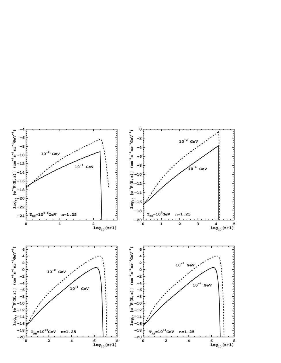
On Fig.5 the integrand of the background spectrum integral, considered in Sec.III is shown as a function of redshift $z$ for several values of the parameter $T_{RH}$. The inclusion of the absorption effects leads to an appearing of the additional factor in this integral:

$$S(E)=\int e^{-\tau(E,z)}\,F(E,z)d\log_{10}(z+1)\;\;\;,$$ (114)

$$\tau(E,z)=\tau_{\nu\tilde{\nu}}(E,z)+\tau_{\nu N}(E,z)\;\;.$$ (115)

Each curve in Fig.5 has a strong cut off on some redshift value. This feature is connected with the existence in our model the minimum value of PBH mass. The PBH mass spectrum is steeply falling function of the mass, so the masses near minimum give a largest contribution to the neutrino background. The moment of their evaporation is, approximately,

$$t_{ev}\approx\frac{\left(M_{PBH}^{min}\right)^{3}}{3\alpha}\;\;,$$ (116)

and the corresponding redshift is determined by the relation

$$z_{ev}+1\approx(z_{eq}+1)\left(\frac{t_{eq}}{t_{ev}}\right)^{1/2}\;\;\;.$$ (117)

Larger masses evaporate at larger times and smaller redshifts. If, for instance, $T_{RH}=10^{10}\;\;\mbox{GeV}$, one has $t_{i}=0.24\cdot 10^{-26}\;\;\mbox{s}$ ; $M_{i}=7,5\cdot 10^{10}\;\;\mbox{g}$ , $z_{ev}\sim 10^{7}$. So, at $T_{RH}=10^{10}\;GeV$ the redshifts of order of $10^{7}$ give a largest contribution to the neutrino background (if there is no neutrino absorption; the absorption effects are essential just near $z\sim 10^{7}$, and, as one can see from the figure, the actual $z$-dependences of the integrand have peak values at $z\sim(2\div 3)\cdot 10^{6}$, depending on a neutrino energy).

The cut off value $z_{ev}$ strongly depends on $T_{RH}$:

$$z_{ev}\sim\frac{1}{\sqrt{t_{ev}}}\sim\left(M_{BH}^{min}\right)^{-3/2}\sim t_{i}^{-3/2}\sim T_{RH}^{3}\;\;.$$ (118)

Again, this estimate does not take into account the absorption effects. The real situation is seen on the figure. In particular, at $T_{RH}>10^{10}\text{ GeV}$ this cut off is the same for all $T_{RH}$ values, as a result of a strong absorption at $z\gtrsim 3\cdot 10^{6}$.

On Figs.6,7 spectra of electron neutrino background are shown separately for several channels of the neutrino production. One can see from Fig.6 that 1) the contribution to the summary background from the direct $\nu_{e}$ emission is, at $T_{RH}\gtrsim 10^{9}\text{GeV}$, absolutely dominant for $E\gtrsim 1\text{ MeV}$ and 2) the relative importance of different channels changes with an increase of $T_{RH}$. It is seen also that at $T_{RH}\gtrsim 10^{9}\text{GeV}$ the contribution of the quark fragmentation channel is very small at $E\gtrsim 1\text{ MeV}$ $(\lesssim 5\%)$, so the evident underestimation of this channel in our calculation, connected with the neglect of the contribution of heavy quark fragmentations, has (at large $T_{RH}$ values) no particular importance.

Situation with the contribution from quark fragmentations is slightly different at smaller $T_{RH}$ values (see Fig.7). Due to the flattening out of the curve for direct $\nu_{e}$ emission the relative contribution of the fragmentation channel at $E\sim 1\text{MeV}$ grows with an decrease of $T_{RH}$. The highest relative contribution is at $T_{RH}\sim 10^{8.5}\text{GeV}$. At this $T_{RH}$ the minimum value of mass in PBH mass spectrum ($M_{BH}^{min}$) coincides with the threshold of quark evaporations ($m_{thr}\sim 10^{14.1}\text{g}$, according to Fig.1). At further decrease of $T_{RH}$ the relative contribution of quark fragmentations at $E\sim 1\text{MeV}$ fastly decreases and, at some $T_{RH}$ value, it is strictly zero (when, due to correspondingly large $M_{BH}^{min}$ value, the age of the universe is not enough for ”warming-up” the PBHs).

It follows from Fig.7 that at neutrino energies larger than $\sim(5\div 10)\text{MeV}$ the contribution of fragmentation channels is negligibly small ( $\lesssim 5\%$). As was mentioned above, the region of smaller neutrino energies is not important for the calculation of spectral index constraints, so some possible underestimation of the quark fragmentation contribution in this region (due to the simplified treatment of them in the present paper) is not sufficient.

Some typical results of calculations of summary electron neutrino background spectra are shown on Figs.8,9. The main features of such spectra have been revealed in previous works [14, 31, 32]: $E^{-3}$ dependence above $100\text{ MeV}$ and the flattening out of the spectra at lower energies. The form of background spectra depends on the form of an initial PBH mass distribution. In refs.[31, 32] the simple power mass spectrum of PBHs containing no cut off (minimum mass value) were used. The behavior of background spectra at low energies in this case is, aside from jet fragmentation contribution, $\sim E^{-1}$ and turnover energy is $\sim 100\text{MeV}$ [31]. In the case of PBH mass spectrum with the cut off the turnover energy depends on $T_{RH}$ [14] (it decreases as $T_{RH}$ increases, as is seen at Fig.8). According to Figs.8,9 the turnover energy is about $1\text{ MeV}$ at $T_{RH}=10^{9}\;\text{ GeV}$. Besides, it was shown in ref.[14] that at low energies the photon background spectra are almost flat and,as is seen in Figs.8,9, the same is also true in the case of the neutrino background spectra.

VI Constraints on the spectral index

For an obtaining of the constraints on the spectral index we use three types of neutrino experiments.

1. Radiochemical experiments for the detection of solar neutrinos. There are data on solar neutrino fluxes from the famous Davis experiment [33] and the $Ga-Ge$ experiment [34]. The basic process used in radiochemical experiments is a charged-current neutrino capture reaction

$$\nu_{e}+A^{N}_{Z}\to e^{-}+A^{N-1}_{Z+1}\;.$$ (119)

In general, the cross section for the neutrino absorption via a bound-bound transition can be calculated using the approximate formula

$$\sigma=\left\{\begin{aligned} &\frac{G_{F}^{2}}{\pi}\left(\langle 1\rangle^{2}+\left(\frac{g_{a}}{g_{v}}\right)^{2}\langle\sigma\rangle^{2}\right)p_{e}E_{e}&\;,\;&E<100MeV\\ &\text{\it const. }&\;,\;&E>100MeV.\end{aligned}\right.$$ (120)

Here, $p_{e}$ and $E_{e}$ are the momentum and the energy of an electron produced in a neutrino capture reaction. Neutrino and electron energies are connected by the relation

$$E_{e}=E-E_{thr}+m_{e}\;.$$ (121)

Stopping of the rise of a neutrino capture cross section (for a bound-bound transition) with neutrino energy is due to influence of a weak nuclear formfactor of the transition. The approximate value of the turnover energy in Eq.(120) is determined from the relations

$$E\sim q_{max}\sim\frac{1}{R_{A}}\sim m_{\pi}\;.$$ (122)

Here, $q_{max}$ is a maximum momentum transfer from a neutrino to the nucleus (in a model with step-like nuclear formfactor), $R_{A}$ is a size of the nucleus.

In the case of the Davis experiment the neutrino capture reaction is

$$\nu+^{37}Cl\to^{37}Ar+e^{-}\;.$$ (123)

Here we took into account the super- allowed transition only, i.e., the transition to the isotopic analog state in ${}^{37}Ar$, for which

$$\langle 1\rangle^{2}=3\;\;,\;\;\langle\sigma\rangle^{2}=0.2\;\;,\;\;E_{thr}\approx 5MeV.$$ (124)

This transition gives dominant contribution to the effect in the detector, in spite of the rather high energy threshold, due to the large value of the Fermi strength $\langle 1\rangle^{2}$.

In the case of the $Ga-Ge$ reaction,

$$\nu+^{71}Ga\to^{71}Ge+e^{-}\;,$$ (125)

the main contribution gives the ground state - ground state transition ($E_{thr}=0.242MeV$). In ${}^{71}Ge$ also there is an isotopic analog state, but its energy is too high, $\sim 9\text{ MeV}$ (it is slightly higher than the particle emission threshold, so this transition is irrelevant). The cross section of the ground state - ground state transition in the reaction (125) is given by the expression [35] (for $E<100\text{ MeV}$)

$$\sigma\cong\frac{G^{2}}{\pi}p_{e}E_{e}\frac{2J_{A}+1}{2J_{B}+1}\cdot\frac{6163.4}{ft}\;.$$ (126)

Here, $J_{A}$ and $J_{B}$ are angular momenta of ${}^{71}Ga$ and ${}^{71}Ge$, respectively, $ft$ value is determined by the half-life time of ${}^{71}Ge$. According to ref.[35] one has

$$J_{A}=\frac{3}{2}\;\;,\;\;J_{B}=\frac{1}{2}\;\;,\;\;\lg ft=4.37\;\;.$$ (127)

The number of target atoms $N^{T}$ in the detectors is about $2.2\cdot 10^{30}$ for the $Cl-Ar$ experiment [33] and $\sim 10^{29}$ for the $Ga-Ge$ experiments [34]. The average statistics is $\sim 1.5\;\text{ captures/day}$ ($Cl-Ar$) and $\sim 1\;\text{ capture/day}$ ($Ga-Ge$). The constraints are calculated using the relation

$$4\pi\cdot N^{T}\cdot 10^{5}\cdot\int S(E)\sigma(E)dE<1.$$ (128)

2. The experiment on a search of an antineutrino flux from the Sun [36]. In some theoretical schemes (e.g., in the model of a spin - flavor precession in a magnetic field) the Sun can emit rather large flux of antineutrinos. LSD experiment [36] sets the upper limit on this flux, $\Phi_{\tilde{\nu}}/\Phi_{\nu}\leq 1.7\%$. In this experiment the neutrino detection is carried out using the reaction

$$\tilde{\nu}_{e}+p\to n+e^{+}\;.$$ (129)

The number of target protons is $\sim 8.6\cdot 10^{28}$ per 1 ton of the scintillation detector, and the obtained upper limit is $0.28$ antineutrino events per year per ton [36]. The cross section of the reaction (129) is well known (see, e.g.,[37]). In particular, in the low energy region ($E\ll m_{p}$) it is given by the formula

$$\sigma(\tilde{\nu}+p+e^{+}+n)=\frac{G^{2}_{F}}{\pi}\left(1+3\left(\frac{g_{a}}{g_{v}}\right)^{2}\right)p_{e}E_{e},$$ (130)

$$E_{e}=E-(m_{n}-m_{p}).$$ (131)

The threshold of this reaction is given by the relation

$$E_{thr}=m_{n}-m_{p}+m_{e}\approx 1.8\mbox{ MeV}.$$ (132)

The cross section of the reaction (129) grows with the neutrino energy up to $E\sim 2\;GeV$, and is a constant ($\sim 0.5\cdot 10^{-38}\;cm^{2}$) at larger energies.The product of this cross section and a PBH antineutrino background spectrum has the broad maximum at $E\sim 100MeV$. The constraint is determined from the condition that the calculated effect in the LSD detector is smaller than the upper limit obtained in ref.[36].

3. The Kamiokande experiment on a detection of atmospheric electron neutrinos [38]. In this experiment the electrons arising in the reaction

$$\nu_{e}^{atm}+n\to p+e^{-}$$ (133)

in the large water Cherenkov detector were detected and, moreover, their energy spectrum was measured. This spectrum has a maximum at the energy about $300MeV$. The spectrum of the atmospheric electron neutrinos is calculated(see, e.g.,[39]) with a very large accuracy (assuming an absence of the neutrino oscillations) and the experimentally measured electron spectrum coincides, more or less, with the theoretical prediction. The observed electron excess at $E\sim 100MeV$ (which is a possible consequence of the oscillations) is not too large. We use the following condition for an obtaining the our constraint : the absolute differential intensity of the PBH neutrino background at the neutrino energy $E\sim 0.3GeV$ cannot exceed the theoretical differential intensity of the atmospheric electron neutrinos at the same energy (otherwise the total number of electrons in the detector and the energy spectrum of these electrons must be different from the observed ones).

VII Results and discussions

Fig.10,11 shows our results for the spectral index constraints. It is seen that the best constraints are obtained using the Kamiokande atmospheric neutrino data and the LSD upper limit on an antineutrino flux from the Sun.

It appears that the spectral index constraints obtained in the present work are not stronger than the corresponding constraint following from COBE data (see Eq.(79)). One should remember, however, that our approach directly constrains the perturbation amplitude $\sigma_{H}(M_{h})$ rather than the spectral index. Comoving length scales of perturbations, for which we constrain the amplitude, are very small in comparison with the size of present horizon. For example, if $T_{RH}\sim 3\cdot 10^{8}\text{ GeV}$ the minimum PBH mass value is about $10^{14}\text{ g}$. In this case the time of PBH formation is

$$t_{i}\sim\frac{M_{BH}^{min}}{M_{pl}}t_{pl}\sim 10^{-24}\text{ s},$$ (134)

the corresponding scale factor is, according to Eq.(43), about$\sim 10^{22}$, and for the comoving length scale one obtains

$$\lambda_{i}\sim\frac{ct_{i}}{a}\sim 10^{-9}\text{ pc}.$$ (135)

It is clear that the normalization on COBE data has sense only if it is assumed that the spectral index is independent on scale. The curves of Fig.10,11 were obtained using just this assumption; it is very easy to calculate from them the corresponding constraints on $\sigma_{H}(M_{h})$.

For a demonstration of the sensitivity of these results to a chosen $\Omega_{\Lambda}$-value we calculate the constraints for two extreme $\Omega_{\Lambda}$-values, for which the parametrization for $f_{S}^{(0)}$ (Eq.(76)) is still valid. It is clear that some weakening of the constraint with an increase of $\Omega_{\Lambda}$ is due to the corresponding decrease of values of the function $\sigma_{H}(M_{h})$ entering the initial PBH mass spectrum (see Eq.(20)). This decrease of $\sigma_{H}(M_{h})$ takes place solely due to the dependence of $f_{S}^{(0)}$ on $\Omega_{\Lambda}$ (see Eq.(76)).

The behavior of the constraint curve $n(T_{RH})$ is sharply different from that was obtained in ref. [15] (authors of ref. [15] used the initial PBH mass function following from the near critical collapse scenario with a domination of the earliest epoch of PBHs formation, and diffuse extragalactic photon data).

The slight bend at $T_{RH}\sim 10^{10}\text{GeV}$ of the constraint curves (Fig.10) is an effect of a neutrino absorption in the space. Constraint based on the atmospheric neutrino experiment is especially sensitive to the absorption because neutrinos of larger energies (in average) are responsible for it.

Flattening out of the constraint curve $n(T_{RH})$ with increase of $T_{RH}$ is connected with the dependence $M_{BH}^{min}(T_{RH})$. According to the relations (34,52,113), the minimum value of PBH mass in the initial mass spectrum is inversely proportional to $T_{RH}^{2}$. More exactly, the relation between $M_{BH}^{min}$ and $T_{RH}$ is

$$M_{BH}^{min}(g)=\frac{7.2\cdot 10^{30}}{(T_{RH}/1GeV)^{2}}.$$ (136)

At small $T_{RH}$ the minimum value of PBH mass in the initial PBH mass spectrum is large and the neutrino background is dominated by the evaporations at recent epochs. In opposite, at large $T_{RH}$, when $M_{BH}^{min}$ is small, the neutrino background is dominated by the evaporations at earlier times. Thus, using the relation

$$z_{eq}\simeq 2.4\cdot 10^{4}\Omega_{m}h^{2}$$ (137)

and the curves, corresponding to $T_{RH}=10^{9}\text{GeV}$ in Fig.5, one can see that in cases when $T_{RH}>10^{9}\text{GeV}$ the neutrino background is dominated by PBH evaporations during the radiation era.

Introducing, as usual [41], the function $M^{*}(M_{BH}^{min})$ by the formula

$$M^{*}(M_{BH}^{min})=\left[3\alpha(M_{BH}^{min})t_{0}\right]^{1/3}\;,$$ (138)

where $t_{0}$ is the age of the universe, one can easily see that at low $T_{RH}$ (before the flattening out of our $n(T_{RH})$ curve) the inequality $M_{BH}^{min}>M^{*}(M_{BH}^{min})$ takes place while at large $T_{RH}$ one has $M_{BH}^{min}<M^{*}(M_{BH}^{min})$. We remind that $M^{*}$ is the mass of a black hole, formed in the early universe and evaporating today. The turning-point (i.e., the point of a change of the slope of the $n(T_{RH})$ curve) corresponds to the equality $M_{BH}^{min}=M^{*}(M_{BH}^{min})$ and in the case $\Omega_{\Lambda}=0$ it is at $T_{RH}\sim 10^{8}\text{GeV}$. The shift of this turning-point with an increase of $\Omega_{\Lambda}$ is explained by the corresponding increase of an age of the universe:

$$t_{0}=\frac{2}{3H_{0}\sqrt{\Omega_{\Lambda}}}\ln\frac{1+\sqrt{\Omega_{\Lambda}}}{\sqrt{1-\Omega_{\Lambda}}}\;\stackrel{{\scriptstyle\Omega_{\Lambda}\to 0}}{{\longrightarrow}}\;\frac{2}{3H_{0}}\;.$$ (139)

One can compare our spectral index constraints with the corresponding results of ref. [14], where the same initial mass spectrum of PBHs had been used. Some difference in resulting constraints ($\Delta n\sim 0.02$) may be connected simply with the fact that authors of ref. [14] use slightly different formula for $\sigma_{H}(M_{h})$, namely,

$$\sigma_{H}(M_{h})=\sigma_{H}(M_{h\;,0})\left(\frac{M_{h}}{M_{h\;,0}}\right)^{\frac{1-n}{4}}.$$ (140)

In other respects the constraints are quite similar although in ref. [14] they were based on diffuse extragalactic photon background data.

One should note that usually the calculations of these constraints are accompanied by the calculation of the bounds based on requirement that the energy density in PBHs does not overclose the universe at any epoch ($\Omega_{BH}<1$). For a setting of such bounds one must consider the cosmological evolution of the system PBHs + radiation. We intend to carry out these calculations in a separate paper. Estimates show that at large $T_{RH}$ values ($T_{RH}\gtrsim 10^{10}\text{GeV}$) the constraints based on $\Omega_{BH}<1$ are stronger than those based on the neutrino experiments (it is the reason why we did not explore the region $T_{RH}>10^{10}\text{GeV}$ in the present paper).

The neutrino background spectra obtained in the present paper may be useful somewhere else, irrespective of the spectral index constraint problem. The main feature of such spectra at $E\gtrsim 1MeV$ and at $T_{RH}\gtrsim 10^{9}-10^{10}\text{ GeV}$ is the very small contribution ($\lesssim 5\%$) of all secondary channels of the neutrino production at evaporation (except the decay of directly evaporated muons) (see Fig.6). There are two reasons for this: the steepness of the initial PBH mass spectrum and, most essentially, the existence in our model the cut off in this spectrum, i.e., the minimum PBH mass value. Evaporation of PBHs having masses near $M_{BH}^{min}$ gives the dominant contribution in the background, so there is a strong maximum in $z$ distributions at low energies (Fig.5). For example, at $T_{RH}=10^{10}\text{GeV}$ the peak value of $z$ is $\sim 10^{6}$. Neutrino energy $\sim 1\text{MeV}$ corresponds in this case to energy at evaporation $\sim 1\text{TeV}$. For an evaporation of such high energy neutrinos the PBH mass must be $\sim 10^{10}\text{g}$ in the case of direct neutrinos and much smaller in the case of secondary neutrinos (because their energies are much lower in average (see Fig.2)). At the same time, the minimum value of PBH mass in the mass spectrum at $T_{RH}=10^{10}\text{GeV}$ is $\sim 10^{11}\text{g}$. So, it should be clear that, in our example, the secondary neutrinos with $E\sim 1\text{MeV}$ can appear only after the essential evolution of the initial PBH mass spectrum (see Eq.(37) and the detailed discussion of this evolution in ref.[40]). This evolution leads to an increase of the total mass interval and to the corresponding decrease of a PBH number density (per unit mass interval) and, as a result, to a relative smallness of the secondary neutrino flux.

One can compare our results for the neutrino background spectra with those of ref.[31, 32]. According to the conclusions of ref.[32], the secondary neutrino fluxes are larger relatively and even dominant at $E\lesssim 10\text{MeV}$. Similar results were obtained in earlier work [31]. In our model the dominance of secondary neutrino fluxes at $E<10\text{ MeV}$ takes place at some values of $T_{RH}$ only (see Fig.7).

The results for neutrino diffuse background spectra and the constraints on the spectral index obtained here do not take into account the possible existence of the photospheres [42, 43, 44] around a black hole. In studies of photon background spectra two kinds of photospheres should be considered: QCD photosphere (quark-gluon plasma arising from interactions of quarks and gluons before hadronization) and QED photosphere ($e^{+}-e^{-}-\gamma$ plasma, in which directly evaporated photons are processed). As for the latter, in our case one should consider instead the ”electroweak (or neutrino) photosphere” [42] which may form only at extremely high black hole temperatures and, probably, has no influence on the background spectra. QCD photosphere may be more important for the problem. Thus, the recent calculations [44] of instantaneous photon spectra from the model QCD photosphere show that some increase of photon fluxes (in comparison with the usual case when QCD photosphere does not form and photons appear simply through the direct quark fragmentations with subsequent $\pi^{0}$-decays) definitely takes place. For example, according to these calculations, at $T_{BH}=50\text{GeV}$ the peak value of instantaneous photon spectrum increases on a factor $\sim 4$. If it is true and if this increase is the same at all black hole temperatures, the contribution to neutrino background spectra from the quark fragmentations obtained in our calculations must be increased approximately on the same factor.

FIG. 1.: The function $\alpha(m)$ counting the degrees of freedom of the PBH radiation ($m$ is an instantaneous value of the PBH mass). Solid line is the present result, dashed line is drawn using Eq.(7) of Ref.[17].

FIG. 2.: Instantaneous electron neutrino spectra from the evaporation of PBH with $T_{BH}=1\text{TeV}$, for several channels of the neutrino production.

FIG. 3.: Instantaneous neutrino spectra from a black hole with a temperature of 100 GeV.

FIG. 4.: Absorption factor for two channels of neutrino absorption and for several values of neutrino energy, as a function of $z$, the redshift corresponding to a moment of the neutrino emission.

FIG. 5.: Redshift dependence of the integrand of the expression (114) for a neutrino background spectrum (with $\Omega_{\Lambda}=0$), for two values of the neutrino energy and for several values of the parameter $T_{RH}$ .

FIG. 6.: Separate contributions to neutrino background spectra from different channels of the neutrino production during PBH evaporation, for fixed values of the parameters $T_{RH}$ and $n$.

FIG. 7.: Separate contributions to neutrino background spectra from two channels of the neutrino production during PBH evaporation, for three different values of $T_{RH}$.

FIG. 8.: Electron neutrino background spectra from PBHs, calculated for several values of reheating temperature. Dashed curve shows the spectrum for $T_{RH}=10^{10}\text{GeV}$, calculated without taking into account the neutrino absorption.

FIG. 9.: Electron neutrino background spectra from PBHs, calculated for several values of the spectral index. Dashed curve shows the theoretical atmospheric neutrino spectrum at Kamiokande site [39] (averaged over all directions).

FIG. 10.: Constraints on the spectral index $n$ as a function of the reheating temperature $T_{RH}$, from three types of the neutrino experiments.

FIG. 11.: Constraints on the spectral index $n$ as a function of the reheating temperature $T_{RH}$, based on the solar $\tilde{\nu}_{e}$ experiment, for two values of $\Omega_{\Lambda}$.