Energetics of Gamma Ray Bursts

Abstract

We determine the distribution of total energy emitted by gamma-ray bursts for bursts with fluences and distance information. Our core sample consists of eight bursts with BATSE spectra and spectroscopic redshifts. We extend this sample by adding four bursts with BATSE spectra and host galaxy R magnitudes. From these R magnitudes we calculate a redshift probability distribution; this method requires a model of the host galaxy population. From a sample of ten bursts with both spectroscopic redshifts and host galaxy R magnitudes (some do not have BATSE spectra) we find that the burst rate is proportional to the galaxy luminosity at the epoch of the burst. Assuming that the total energy emitted has a log-normal distribution, we find that the average emitted energy (assumed to be radiated isotropically) is $\langle E_{\gamma iso}\rangle=1.3^{+1.2}_{-1.0}\times 10^{53}$ ergs (for H₀ = 65 km s^-1 Mpc^-1, $\Omega_{m}=0.3$ and $\Omega_{\Lambda}=0.7$); the distribution has a logarithmic width of $\sigma_{\gamma}=1.7^{+0.7}_{-0.3}$. The corresponding distribution of X-ray afterglow energy (for seven bursts) has $\langle E_{Xiso}\rangle=4.0^{+1.6}_{-1.8}\times 10^{51}$ergs and $\sigma_{X}=1.3^{+0.4}_{-0.3}$. For completeness, we also provide spectral fits for all bursts with BATSE spectra for which there were afterglow searches.

1 Introduction

The recent breakthrough in our understanding of gamma-ray bursts resulted from associating of these events with host galaxies. This association demonstrates that most, and probably all, bursts are at cosmological distances. Whether measured from absorption lines in the continuum of optical transients or emission lines in the host galaxies’ spectra, the redshifts show that the bursts are even further than predicted by the simplest “minimal” cosmological model (Band & Hartmann, 1998). With assumptions about the radiation pattern, the energy radiated by the burst is calculated from the redshifts and the burst fluence. The position of the burst within the host argues for a strong connection between star formation and the burst (Bloom et al., 2001). Many of the galaxies show evidence of vigorous star formation.

We now have a sufficient sample of detected host galaxies to consider various distributions of burst properties which require the distance to the burst. Here we calculate the distributions of the total energy and peak luminosity radiated by the burst and the X-ray energy in the afterglow. The energy scale is a strong constraint on burst scenarios; some proposed sources are insufficient to provide the necessary observed energy. However, the width and shape of the energy distributions are also consequences of the emission process. For example, in the current physical scenario (Narayan et al., 1992; Paczynski & Xu, 1994; Rees & Meszaros, 1994; Sari & Piran, 1997) the gamma-rays are radiated by “internal” shocks resulting from the collision of regions with different Lorentz factors within a relativistic outflow. Thus the total gamma-ray emission may depend on the vagaries of the central source accelerating the outflow. However, the afterglow is attributed to the “external” shock where the outflow collides with the external medium. Thus the afterglow may be a bolometric measurement of the energy content of the relativistic flow. This is the basis of the “patch shell” model’s prediction that the gamma-ray energy distribution should be broader than that of the afterglows (Kumar & Piran, 1999).

To expand the burst sample, we include not only bursts with spectroscopic redshifts, but also bursts for which there are only host galaxy magnitudes. A galaxy magnitude can be mapped into a probability distribution for the burst’s redshift. This mapping requires a model of the host galaxy distribution; competing models are tested by comparing the measured spectroscopic redshifts with the magnitude-derived redshift distribution for those bursts with both a spectroscopic redshift and a host galaxy magnitude. This host galaxy model is intrinsically interesting since it indicates whether the burst rate is proportional to the host galaxy mass or luminosity.

An underlying assumption in our study is that the burst energy and luminosity distributions have not changed over the universe’s lifetime. Similarly, we assume that a burst’s energy or luminosity is uncorrelated with the host galaxy magnitude.

In §2 we present the expected fluence distribution given the assumed lognormal burst energy distribution. §3 describes the sources of the observed $\gamma$-ray and X-ray energy fluxes and fluences. §4 discusses the determination of a burst redshift from a single optical magnitude of the host galaxy. However, galaxy surveys count individual galaxies while the burst rate may be proportional to the mass or luminosity of a galaxy; therefore in §5 we consider the underlying host galaxy luminosity function. The burst $\gamma$-ray and X-ray energy distributions are calculated in §6. Our conclusions are summarized in §7.

2 The Expected Fluence Distribution

Here we present the methodology for modeling the distribution of the total burst energy $E_{\gamma}$ given a set of observed burst fluences. The determination of the distribution of the peak gamma-ray luminosity and of the X-ray afterglow energy are analogous.

We begin by assuming that $E_{\gamma}$ has a log-normal distribution,

$$p(E_{\gamma}\,|\,\langle E_{\gamma iso}\rangle,\sigma_{\gamma})d(\log E_{\gamma})={1\over{\sqrt{2\pi}\sigma_{\gamma}}}\exp\left[-{{(\log(\langle E_{\gamma iso}\rangle)-\log(E_{\gamma}))^{2}}\over{2\sigma_{\gamma}^{2}}}\right]d(\log E_{\gamma})\quad.$$ (1)

Thus the bolometric fluence $F=E_{\gamma}(1+z)/4\pi D_{L}(z)^{2}$ (where $D_{L}(z)$ is the luminosity distance) has the log-normal distribution

$$p(F\,|\,\langle E_{\gamma iso}\rangle,\sigma_{\gamma})d(\log F)={1\over{\sqrt{2\pi}\sigma_{\gamma}}}\exp\left[-{{(\log(\langle E_{\gamma iso}\rangle(1+z)/4\pi D_{L}(z)^{2})-\log(F))^{2}}\over{2\sigma_{\gamma}^{2}}}\right]d(\log F)\quad.$$ (2)

Note that $\sigma_{\gamma}$ is a width in logarithmic space, and the linear change of variables does not affect this width. This probability for the fluence assumes that the redshift is known. If not, then we have to convolve eq. 2 with the probability distribution for the host galaxy redshift, $p_{B}(z\,|\,D_{o})$, where $D_{o}$ is the optical data we have about the redshift (e.g., the measured spectroscopic redshift from spectral lines or the host galaxy magnitude). The resulting probability is

$$p(F\,|\,\langle E_{\gamma iso}\rangle,\sigma_{\gamma})d(\log F)=$$ (3)

$$\int dz\,p_{B}(z\,|\,D_{o}){1\over{\sqrt{2\pi}\sigma_{\gamma}}}\exp\left[-{{(\log(\langle E_{\gamma iso}\rangle(1+z)/4\pi D_{L}(z)^{2})-\log(F))^{2}}\over{2\sigma_{\gamma}^{2}}}\right]d(\log F)\quad.$$

These are the distributions for $E_{\gamma}$ and $F$, regardless of whether these quantities are actually observable. The distributions for the observable bursts must therefore be truncated at the threshold value of the fluence, $F_{T}$, and the overall distribution must be renormalized. Thus

$$p_{\hbox{obs}}(F\,|\,\langle E_{\gamma iso}\rangle,\sigma_{\gamma})={{p(F\,|\,\langle E_{\gamma iso}\rangle,\sigma_{\gamma})\theta(F-F_{T})}\over{\int_{F_{T}}^{\infty}dF\,p(F\,|\,\langle E_{\gamma iso}\rangle,\sigma_{\gamma})\theta(F-F_{T})}}$$ (4)

where $\theta(x)$ is the Heaviside function (1 above $x=0$, and 0 below). Since BATSE triggers on the peak count rate $C_{\hbox{max}}$ and not the fluence, the threshold fluence $F_{T}$ is the observed fluence divided by $C_{\hbox{max}}/C_{\hbox{min}}$, where $C_{\hbox{min}}$ is the threshold count rate (i.e., the minimum peak count rate at which BATSE would have triggered). Thus $F_{T}$ and $p_{\hbox{obs}}(F\,|\,\langle E_{\gamma iso}\rangle,\sigma_{\gamma})$ vary from burst to burst. For calculations of the X-ray afterglow energy the X-ray detectability threshold must be used instead of $F_{T}$. The likelihood is the product of these probabilities evaluated with each burst’s observed properties (fluence, redshift, etc.) for all bursts in the sample. By maximizing this likelihood we find the preferred values and confidence ranges for $\langle E_{\gamma iso}\rangle$ and $\sigma_{\gamma}$ (or the equivalent for the X-ray afterglow). Note that the selection effect introduced by observing bursts at different redshifts—only intrinsically bright high redshift bursts are observable—while the detector threshold varies is mitigated by truncating the probability distribution for the observable fluence at the threshold value.

3 $\gamma$-Ray and X-Ray Data

We consider the sample of GRBs with observed optical afterglows and with detected host galaxies, whether or not a redshift has been measured, for bursts between 1997 January and 2000 June (CGRO’s untimely demise). To obtain a uniform estimate of the $\gamma$-ray energy fluence we consider only those bursts detected by BATSE. The bursts with BATSE data and a spectroscopic redshift are GB970508, GB970828, GB971214, GB980425, GB980703, GB990123, GB990506, GB990510, and GB991216; however, GB980425 is exceptional because of its possible association with a supernova in a relatively nearby galaxy and we do not include it in our sample. The bursts with BATSE data and only an R magnitude for its host galaxy are GB971227, GB980326, GB980329, and GB980519. In addition, both R magnitudes and spectroscopic redshifts but no BATSE data are available for GB970228, GB980613, and GB990712. For GB990510 there is currently a spectroscopic redshift but no host galaxy R magnitude. Thus, there are eight bursts for which we can calculate the total emitted energy, and another four for which we can calculate a range of possible energies. There are ten bursts for which we have both spectroscopic redshifts and a host galaxy R magnitude; from these ten we determine a model of the host galaxy population, as described below.

To calculate the total gamma-ray energy emitted by a burst we need the observed gamma-ray fluence. We determine the fluence of a given burst by fitting the spectrum accumulated over the time segment during which there was detectable emission. For strong bursts we use spectra from BATSE’s Spectroscopy Detectors (SDs), while for weak bursts we fit spectra from BATSE’s Large Area Detectors (LADs). Since BATSE consisted of 8 modules, each with an SD and an LAD, more than one detector observed each burst. For strong bursts we choose the SD with the smallest burst angle (the angle between its normal and the burst) and with a gain sufficiently high to cover the 30–1000 keV energy band (the SDs were operated at different gains). A typical SD spectrum provides $\sim 200$ usable energy channels. For weak bursts we use the LAD with the highest count rate which almost always had the smallest burst angle.

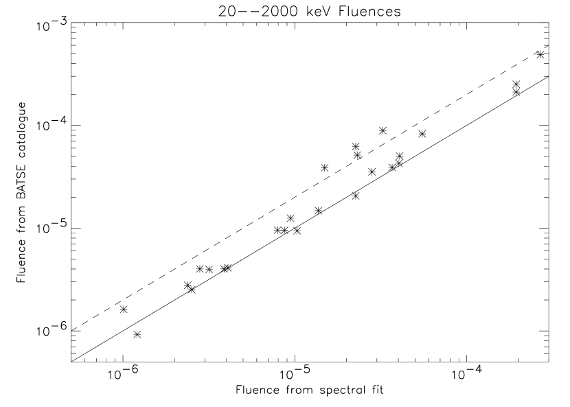
Figure 1: Comparison between the 20–2000 keV fluences (in erg cm^-2) from the BATSE catalog and from integrating the spectral fits in the table over energy and time. The fluences are equal along the solid line while along the dashed line the catalog fluences are twice as great as the fluences derived from the spectral fits.

These spectra were fitted with the “Band function” Band et al. (1993), which consists of a low energy power law cut off by an exponential, $N_{E}=N_{0}(E/100\hbox{ keV})^{\alpha}\exp[-E/E_{0}]$ ph s^-1 keV^-1 cm^-2, which merges smoothly with a high energy power law, $N_{E}\propto E^{\beta}$. The parameters of the resulting fits are given in the 2nd–5th columns of Table 1. The energy fluence $F_{\gamma}$ (6th column of the table) is obtained by integrating this fit over the energy band 20–2000 keV and over the time for which there was detectable emission (the 10th column). This is the energy band of the fluences provided by the BATSE catalogue. In most cases the fluence in this energy band is very nearly the bolometric fluence, and thus no k-corrections are necessary to calculate the energies for bursts at different redshifts (the k-correction compensates for the redshift shift in the energy band between the emitter and the detector). In this table we provide for completeness spectral fits and fluences for all the bursts observed by BATSE which were localized after 1997 January. Figure 1 compares the 20–2000 keV fluences provided by the BATSE catalogues and calculated here; as can be seen, the BATSE catalogue values are somewhat larger than the fluences resulting from spectral fits. Note that there are host galaxy observations for only 12 of the bursts in this table; these 12 burst comprise our “BATSE redshift sample.”

As described above, for each burst we need the threshold fluence, the minimum fluence at which BATSE would have triggered. This is derived by equating the ratios of the observed and threshold fluences and peak count rates: $F_{T}=F/[C_{\hbox{max}}/C_{\hbox{min}}]$. The online BATSE catalog provides $C_{\hbox{max}}/C_{\hbox{min}}$ for some bursts, but values are missing for many bursts because of data gaps. For bursts without a catalog value we have estimated $C_{\hbox{max}}/C_{\hbox{min}}$ from the light curves.

In addition to the energy emitted by the burst (mostly in gamma-rays), significant emission occurs during the first few hours of the afterglow (mostly in X-rays). We estimate this energy (excluding the prompt X-ray emission during the burst) using the observed late (few hours) X-ray flux in the 2–10 keV band and assuming this emission decays as a power law with the index $\delta_{x}$ shown in Table 1 over the period 100 to $10^{5}$ seconds after the burst.

4 Host Galaxy Redshift Distribution

The methodology presented in §2 requires $p_{B}(z\,|\,D_{o})$, the probability that the burst redshift has a given value. Thus far redshift information has been derived from the associated host galaxies. Clearly, if we know the spectroscopic redshift $z_{0}$ then $p_{B}(z\,|\,D_{o})=\delta(z-z_{0})$. However, spectroscopic redshifts are not available for some of the host galaxies. For these host galaxies we derive a redshift probability distribution with a finite width from their observed single-band magnitudes.

The use of photometry to derive galaxy redshifts has flourished during the past 5 years (e.g. Connolly et al. (1995); Sawicki et al. (1997); Driver et al. (1998); Fernandez-Soto et al. (1999); Arnouts et al. (1999)). Redshifts are now commonly determined to an accuracy of 10% (e.g., Csabai et al. (1999)) using multi-band photometry (usually 4 to 6 bands). Multi-band photometry is therefore an economical method of determining redshifts. Unfortunately, most GRB hosts have been observed in only a single band (typically $R$).

It may seem futile to try to determine the redshift of a galaxy from a single band. Galaxies span a large range in stellar masses (i.e., luminosities) and therefore galaxies of a given magnitude are found at virtually any redshift (c.f., Driver (1999)). On the other hand, since the volume element $dV/dz$ peaks at around $z=1-2$ (for reasonable cosmologies) and galaxies formed stars at a higher rate at $z>1$ (and consequently were brighter than at present), we expect a high probability that the average galaxy inhabited the $1<z<2$ region for not too faint magnitudes. Here we use the Hubble Deep Field (HDF) to derive a galaxy redshift distribution at different observed magnitudes. With this distribution we then determine a probability distribution of the host galaxies’ redshift based on their observed optical magnitudes. Our methodology permits us to consider different redshift distributions corresponding to different models of the host galaxy population (e.g., the burst rate is proportional to the galaxy luminosity); we test the hypotheses about the host galaxies by determining whether the model redshift distributions are consistent with the host galaxies with spectroscopic redshifts. We use only observations from the HDF, the deepest available survey, in order not to complicate our analysis with theoretical prejudices in merging results from different surveys. Note that we only require the distribution of redshifts at a given magnitude, and thus as long as a redshift is determined for every galaxy at a given magnitude in the survey field, the HDF will suffice.

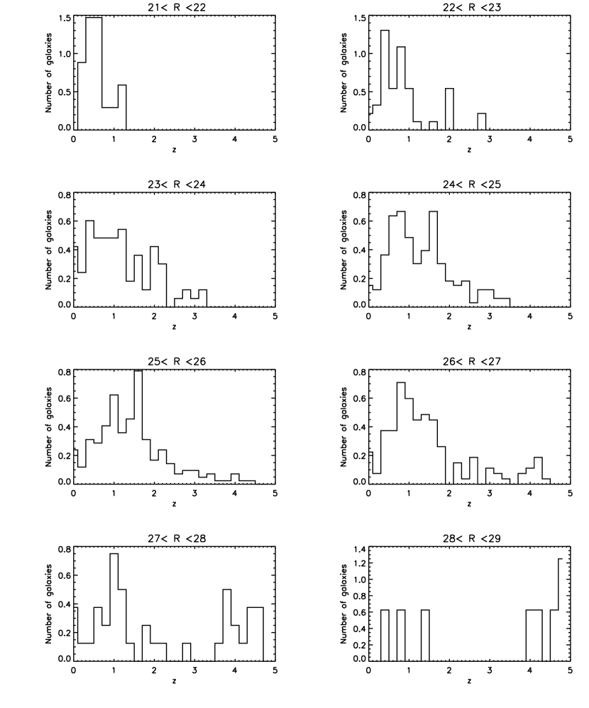
Figure 2: The redshift distribution of galaxies in the $R$ band from the HDF.

Spectroscopic redshifts have thus far not been determined for all the HDF galaxies. However, the available multi-band photometric redshifts (accurate to 10%) will suffice. We have used the HDF catalog from Driver (1999), to which the reader is referred for a full description of the sample and the expected accuracy of the photometric redshifts. In Fig. 2 we show the galaxy redshift distribution as a function of apparent $R$ magnitude, where we have transformed the HST F606W magnitudes into cousins $R$ magnitudes. As expected, $R<26$ galaxies are systematically more common at $z<2$ than at higher redshifts.

When normalized, the distributions in Fig. 2 provide the galaxy redshift probability distributions in a given $R$ magnitude band. Thus the HDF provides $p_{\hbox{HDF}}(z\,|\,f_{R})$—$f_{R}$ is the energy flux corresponding to an R magnitude—from which we derive $p_{B}$ for those bursts without a spectroscopic redshift. Galaxy surveys weight each detected galaxy equally. However, the burst rate may not be the same for each galaxy, and thus we have to weight the galaxies in the HDF based on a model of burst occurrence. To determine how to weight $p_{\hbox{HDF}}$ we have to analyze the origin of this probability: it is the normalized product of the comoving volume per redshift, $dV/dz$, times the galaxy density at $L_{R}$ per comoving volume, $n(L_{R},z)$. $L_{R}$ is the luminosity over the band in the burst’s frame that redshifted into the $R$ band in the observer’s frame; this band varies with redshift. Note that we do not need k-corrections for $L_{R}$ since the density is for those galaxies which provide us with the observed $f_{R}$ in the $R$-band in our frame. Thus

$$p_{\hbox{HDF}}(z\,|\,f_{R})dz={{n(L_{R}=4\pi D_{L}^{2}f_{R},z){{dV}\over{dz}}dz}\over{\int n(L_{R}=4\pi D_{L}^{2}f_{R},z){{dV}\over{dz}}dz}}\quad.$$ (5)

We consider four models. First, we use $p_{\hbox{HDF}}$ as $p_{B}$; every galaxy has an equal probability of hosting a burst. This is inconsistent with most burst scenarios, but serves as a useful null hypothesis.

Second, we assume that the burst rate is proportional to the mass of the galaxy. This corresponds to a scenario where the burst occurs long after the progenitor was formed, and thus the progenitor population is (approximately) proportional to the galaxy’s mass. In this case $p_{B}$ is $p_{\hbox{HDF}}$ weighted by the luminosity the galaxy would have today in the R-band. Thus both a k- and an e-correction are required, where the e-correction compensates for the evolution in the galaxy’s spectrum. Note that these k- and e-corrections are not applied to $p_{\hbox{HDF}}$ but only to the weighting. Thus $p_{B}\propto L_{R}K(z)E(z)p_{\hbox{HDF}}(z\,|\,f_{R})$ where $K(z)$ is the k-correction which references $L_{R}$ (the luminosity in the band at the host galaxy’s redshift which is redshifted into today’s R-band) to today’s R-band and $E(z)$ is the e-correction which maps the R-band luminosity of a galaxy at the host’s redshift to the R-band luminosity it would have at present.

Third, we assume that the burst rate is proportional to the galaxy’s intrinsic luminosity at the time of the burst. This corresponds to scenarios where the burst occurs very soon after the progenitor forms. Thus, if the luminosity per mass was greater in the past as a result of increased star formation, then the burst rate should also increase. This is admittedly an oversimplification of a galaxy’s evolutionary history. For this model $p_{B}\propto L_{R}K(z)p_{\hbox{HDF}}(z\,|\,f_{R})$ where, once again, $K(z)$ is the k-correction which references $L_{R}$ (the luminosity in the band which is redshifted into today’s R-band) to today’s R-band.

Fourth, we model the star formation rate for a given model by weighting the second model, where the burst rate is proportional to the galaxy mass, by the cosmic redshift-dependent star formation rate. This rate rises rapidly with redshift to $z\sim 1$, and then levels off, e.g. citeH+98.

Note that the $p_{B}$ for each of these different models needs to be renormalized given the model-dependent weightings.

Whenever we need to compute a k and/or e–correction in any of the above scenarios, we have used the set of synthetic stellar populations developed in Jimenez et al. (1998). The star formation rate is modelled as a declining exponential, with e-folding ($\tau$) time depending on the morphological type. In particular, we used the following values: $\tau=1$, 3, 5 and $\inf$ for E/S0, Sab, Scd and Irr types respectively. We kept the metallicity fixed at the solar value during the whole evolution of the galaxy and chose $z=4$ as the redshift of formation – starting point of the star formation – for all galaxies. This modeling of galaxies is, indeed, overly simplistic, but it is sufficient for our purposes since we do not require to be precise by more than 0.5 magnitudes when computing the k+e corrections.

5 Testing the Host Galaxy Models

We can test the different models for the host galaxy population using the bursts with both spectroscopic redshifts and host galaxy R magnitudes. We compare the likelihoods using the various models. However, the probability used in these likelihoods is the probability that we would determine the redshift that was indeed observed, not the probability that a host galaxy with a given R magnitude would have a particular redshift. For the telescope which determined the redshift there are redshift windows in which it would not have been able to make this determination. For example, for the Keck observations the redshift is difficult to determine between $z=$1.3, when O[II] is redshifted out of the spectrum, and $z=$2.5, when Ly$\alpha$ is blue shifted in. Thus in the likelihood we should use $p\propto h(z)p_{B}$, where $h(z)$ is the probability of determining a particular value of the redshift; however, including the redshift windows applicable to each observation is beyond the scope of this paper. Note that by modifying the distribution of host galaxy redshifts, whether observable or not, for a given R magnitude into the distribution of host galaxies which are actually observable, we avoid the selection effect resulting from the easier detectability of bright host galaxies.

The resulting likelihood is

$$\Lambda=\prod_{i}{{h(z_{i})p_{B}(z_{i}\,|\,f_{R,i})}\over{\int dz\,h(z_{i})p_{B}(z_{i}\,|\,f_{R,i})}}\quad.$$ (6)

We find that $\Lambda=10^{-3}$ for the model where the burst rate is constant per galaxy, $\Lambda=3\times 10^{-4}$ when the burst rate is proportional to the galaxy mass, $\Lambda=10^{-2}$ when the burst rate is proportional to the galaxy luminosity, and $\Lambda=10^{-4}$ for the model where the burst rate is proportional to the product of the galaxy mass and the cosmic star formation rate. Thus the third model is preferred; we will use the corresponding $p_{B}$ in adding the four bursts with only host galaxy R magnitudes to the sample with spectroscopic redshifts.

6 The Burst Energy Distributions

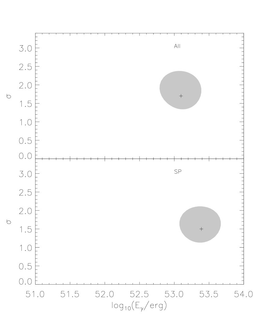
Figure 3: The 70% confidence likelihood contour plot for total burst energy $\langle E_{\gamma iso}\rangle$ and its variance $\sigma_{\gamma}$ (see text) in the 20–2000 keV band when using the 8 bursts with spectroscopic redshifts (top panel) and when adding to these 8 bursts the 4 GRBs with only host galaxy magnitudes (bottom panel).

We first estimate the characteristic isotropic gamma-ray energy ($\langle E_{\gamma iso}\rangle$) and its spread ($\sigma_{\gamma}$) in the 20–2000 keV band. The result is presented in Figure 3. The upper panel shows the likelihood contour corresponding to 70% confidence using only the 8 GRBs with spectroscopic redshifts, while the bottom panel shows the same contour level but with the additional 4 GRBs with statistical redshifts. Therefore, the preferred value for $\langle E_{\gamma iso}\rangle$ is $1.3^{+1.2}_{-1.0}\times 10^{53}$ erg with $\sigma_{\gamma}=1.7^{+0.7}_{-0.3}$. Note that there is no need to k-correct the $\gamma$-ray data in this case because the 20–2000 keV band already contains most of the energy of the GRB.

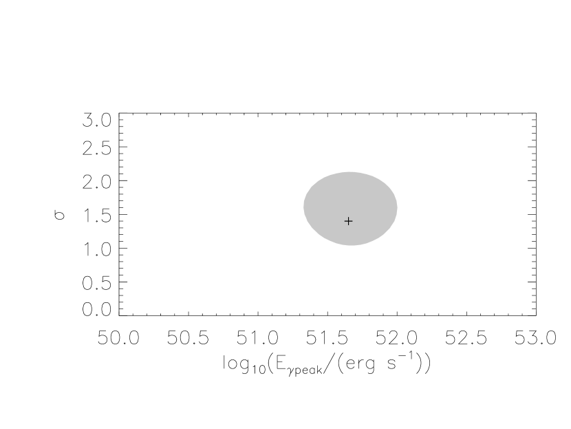
Figure 4: The 70% confidence likelihood contour plot for the peak burst luminosity $\langle L_{\gamma iso}\rangle$ and $\sigma_{L}$ in the 50–300 keV band. Note that in this case we have k-corrected the data from Table 1 using the spectral fits provided in the table.

Similarly we derive the peak luminosity $\langle L_{\gamma iso}\rangle$ in the 50–300 keV band. In this case we apply a k-correction to the data using the spectral fits described in Table 1. Figure 4 shows the 70% confidence contour plot using all the GRBs in our sample. We find $\langle L_{\gamma iso}\rangle=4.6^{+5.4}_{-2.5}\times 10^{51}$ erg s^-1 with $\sigma_{L}=1.4^{+0.7}_{-0.4}$.

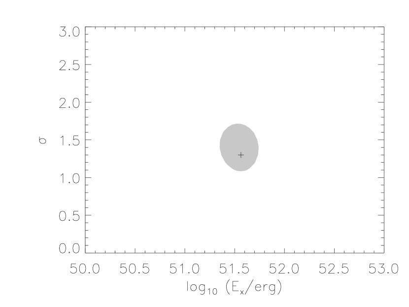
Figure 5: The 70% confidence likelihood contour plot for the total afterglow X-ray energy $\langle E_{Xiso}\rangle$ and $\sigma_{X}$. We integrated the X-ray flux between 100 and $10^{5}$ seconds after the burst in the 2–10 keV band and applied a corresponding k-correction assuming a spectrum $\propto\nu^{-0.75}$.

Finally, we find the average energy of the X-ray afterglow. To homogenize the observations, we integrate the X-ray emission between 100 and 10⁵ seconds after the burst using the best fitting power law to the observed light curve (slopes for the different light curves are given in Table 1). Figure 5 shows the $1\sigma$ contour plot when the 7 GRBs with X-ray light curves are considered. Here we find that $\langle E_{Xiso}\rangle=4.0^{+1.6}_{-1.8}\times 10^{51}$ erg and $\sigma_{X}=1.3^{+0.4}_{-0.3}$.

7 Discussion and Conclusions

We have determined the distributions of the total burst energy, the peak burst luminosity and the total X-ray afterglow energy for a sample of bursts with either spectroscopic redshifts or host galaxy R magnitudes. These distributions reflect the physics of the burst process.

We have found that the best model for the burst rate is proportional to the host galaxy luminosity and not to the host size. This result provides further support to the proposition that the bursts are associated with star formation. Star forming galaxies are brighter than other galaxies with the same size.

It seems that $\langle E_{\gamma iso}\rangle$ is slightly broader than $\langle E_{Xiso}\rangle$, but within the 70% confidence both distributions are compatible with having the same width. However, inspection of the data points shows that X-ray energy of one burst—GRB970508—significantly broadens the X-ray distribution; otherwise the X-ray distribution would be much narrower than the gamma-ray distribution. Thus we must conclude that the data are insufficient to determine conclusively the width of the luminosity functions, although there is a trend for the X-ray distribution to be narrower than the ${\gamma}$ distribution.

The ratio between the widths of the gamma-ray and the X-ray luminosity functions is particularly important as far as the physics of the physical processes within the “inner engine.” A ratio of order unity suggests that the “inner engine” emits a rather uniform flow with no significant angular variation on an angular scale of few degrees (corresponding to the width seen several hours after the burst while the X-rays are emitted). On the other hand, a large $\sigma_{\gamma}/\sigma_{X}$ would support the “patchy shell” model(Kumar & Piran, 1999) which predicts that the gamma-ray energy emitted during the GRB has a significantly wider distribution than the X-ray energy emitted during the afterglow, $\sigma_{\gamma}>\sigma_{X}$. In this model, there are mass fluctuations on the shells whose collisions produce the internal shocks which subsequently radiate the observed gamma-rays. Thus the gamma-ray intensity should vary greatly with the observer’s angle. On the other hand, the afterglow results from the decelerating external shock, and the observer sees a much larger solid angle of the relativistic outflow in the afterglow than in the burst itself. Thus there are smaller fluctuations in the afterglow intensity with observer angle. Finally $\sigma_{\gamma}/\sigma_{X}<1$ would be indicative of extremely large variations (from one burst to the other) in the circumstellar matter surrounding the GRBs. The data are sufficient to rule out this third possibility, but cannot distinguish with confidence between the first and second, although the trend is toward favoring the “patchy shell” model.

It is interesting to compare our results with the energy distribution determined for the whole GRB sample. Schmidt (1999) finds for a broken power law distribution that the energy of the break is $1.2\times 10^{53}$ ergs, which is very close to our average energy. However, the average energy in Schmidt’s distribution is a factor of $\sim 5$ smaller than this break energy. This can be explained by the fact that afterglow can be observed only for the more luminous bursts for which we can determine an exact position.

Finally we note that we have presented here a new methodology for obtaining the luminosity function of a sample for which the magnitude is known but there are no redshift measurements. This method can be best applied to other populations that like GRBs have an intrinsically wide luminosity function. While a galaxy’s optical magnitude does not provide a reliable distance measure for a single object, is should be sufficiently reliable when analyzing a large sample. This method should be tested on other samples in the future.

This methodology can be used wherever burst distances and energies are required. For example, a burst sample with known distances is required to calibrate proposed correlations between the burst energy and the frequency–dependent lags in pulses (Fenimore & Ramirez–Ruiz, 2000) or light-curve variability (Norris et al., 2000).

This research was supported in part by a US-Israel BSF. The work of David Band was performed under the auspices of the U.S. Department of Energy by the Los Alamos National Laboratory under Contract No. W-7405-Eng-36.

Table 1: Main properties of the sample of Gamma Ray Bursts.

Name	$N_{0}$	$\alpha$	$\beta$	$E_{0}$ (keV)	$F_{\gamma}$ (erg cm-2)	$F_{\gamma peak}$ (erg cm-2 s-1)	$\delta_{x}$	$F_{x}$ (erg cm-2 s-1)	$t$ (s)	$R_{\rm gal}$	$z_{\rm obs}$	$z_{\rm est}$
970111	$7.86\times 10^{-2}$	$-0.533$	$\cdots$	106.56	$4.07\times 10^{-5}$	$\cdots$	$\cdots$	$\cdots$	35.36	$\cdots$	$\cdots$	$\cdots$
970228	$\cdots$	$\cdots$	$\cdots$	$\cdots$	$\cdots$	$2.15\times 10^{-6}$	$\cdots$	$\cdots$	$\cdots$	24.6	0.695	0.8
970508	$1.73\times 10^{-3}$	$-1.191$	$-1.831$	480.84	$5.54\times 10^{-6}$	$7.38\times 10^{-7}$	$-1.2$	$3.9\times 10^{-7}$	23.44	25.8	0.835	1.2
970616	$4.99\times 10^{-3}$	$-1.464$	$-2.549$	296.91	$4.03\times 10^{-5}$	$\cdots$	$\cdots$	$\cdots$	203.68	$\cdots$	$\cdots$	$\cdots$
970815	$4.17\times 10^{-3}$	$-1.094$	$-2.802$	113.25	$1.37\times 10^{-5}$	$\cdots$	$\cdots$	$\cdots$	183.59	$\cdots$	$\cdots$	$\cdots$
970828	$1.15\times 10^{-2}$	$-0.704$	$-2.072$	229.74	$9.60\times 10^{-5}$	$3.01\times 10^{-6}$	$-1.0$	$1.82\times 10^{-6}$	146.59	24.5	0.958	0.8
971024	$9.72\times 10^{-3}$	0.185	$-3.881$	40.93	$2.38\times 10^{-6}$	$\cdots$	$\cdots$	$\cdots$	97.82	$\cdots$	$\cdots$	$\cdots$
971214	$7.23\times 10^{-3}$	$-0.783$	$-2.574$	155.96	$9.44\times 10^{-6}$	$2.28\times 10^{-6}$	$-1.6$	$1.31\times 10^{-6}$	45.45	26.2	3.412	1.2
971227	$1.06\times 10^{-2}$	$-1.440$	$-4.198$	112.03	$1.21\times 10^{-6}$	$3.37\times 10^{-6}$	$\cdots$	$\cdots$	6.94	25.0	$\cdots$	1.2
980109	$9.34\times 10^{-3}$	$-0.428$	$-2.291$	62.65	$4.08\times 10^{-6}$	$\cdots$	$\cdots$	$\cdots$	42.97	$\cdots$	$\cdots$	$\cdots$
980326	$2.11\times 10^{-2}$	$-1.327$	$-4.335$	77.19	$9.22\times 10^{-7}$	$8.00\times 10^{-7}$	$\cdots$	$\cdots$	4.01	25.3	$\cdots$	1.2
980329	$2.58\times 10^{-2}$	$-0.964$	$-2.431$	235.65	$5.51\times 10^{-5}$	$1.15\times 10^{-5}$	$-1.34$	$0.56\times 10^{-6}$	50.15	26.3	$\cdots$	1.2
980425	$4.70\times 10^{-3}$	$-1.266$	$\cdots$	161.20	$3.87\times 10^{-6}$	$\cdots$	$\cdots$	$\cdots$	37.41	14.3	0.0085	0.01
980519	$4.79\times 10^{-3}$	$-1.352$	$\cdots$	315.94	$1.03\times 10^{-5}$	$2.98\times 10^{-6}$	$\cdots$	$\cdots$	56.35	24.7	$\cdots$	0.8
980613	$\cdots$	$\cdots$	$\cdots$	$\cdots$	$\cdots$	$3.87\times 10^{-7}$	$-1.6$	$0.55\times 10^{-6}$	$\cdots$	23.85	1.096	0.8
980703	$4.41\times 10^{-3}$	$-1.314$	$-2.396$	370.26	$2.26\times 10^{-5}$	$1.62\times 10^{-6}$	$-1.67$	$1.27\times 10^{-6}$	102.37	22.8	0.966	0.6
980706	$1.50\times 10^{-3}$	$-1.112$	$\cdots$	$5000.0$	$2.31\times 10^{-5}$	$\cdots$	$\cdots$	$\cdots$	72.81	$\cdots$	$\cdots$	$\cdots$
990123	$2.62\times 10^{-2}$	$-0.900$	$-2.476$	549.51	$2.68\times 10^{-4}$	$1.11\times 10^{-5}$	$-1.6$	$8.98\times 10^{-6}$	104.61	24.3	1.600	0.8
990506	$1.51\times 10^{-2}$	$-1.370$	$-2.152$	449.78	$1.94\times 10^{-4}$	$\cdots$	$\cdots$	$\cdots$	220.38	25.0	1.2	$\cdots$
990510	$7.96\times 10^{-3}$	$-1.275$	$-2.670$	174.24	$2.26\times 10^{-5}$	$5.02\times 10^{-6}$	$\cdots$	$\cdots$	103.84	$\cdots$	1.619	$\cdots$
990712	$\cdots$	$\cdots$	$\cdots$	$\cdots$	$\cdots$	$\cdots$	$\cdots$	$\cdots$	$\cdots$	22.0	0.43	0.40
990806	$8.91\times 10^{-3}$	$-0.658$	$-2.261$	109.09	$2.51\times 10^{-6}$	$\cdots$	$\cdots$	$\cdots$	12.71	$\cdots$	$\cdots$	$\cdots$
991014	$1.16\times 10^{-2}$	$-0.754$	$-2.190$	84.65	$1.01\times 10^{-6}$	$\cdots$	$\cdots$	$\cdots$	5.093	$\cdots$	$\cdots$	$\cdots$
991105	$2.16\times 10^{-3}$	$-1.734$	$\cdots$	363.49	$2.80\times 10^{-6}$	$\cdots$	$\cdots$	$\cdots$	34.28	$\cdots$	$\cdots$	$\cdots$
991208	$\cdots$	$\cdots$	$\cdots$	$\cdots$	$\cdots$	$\cdots$	$\cdots$	$\cdots$	$\cdots$	$\cdots$	0.706	$\cdots$
991216	$1.29\times 10^{-1}$	$-1.234$	$-2.184$	414.83	$1.94\times 10^{-4}$	$\cdots$	$\cdots$	$\cdots$	24.96	26.9	1.02	$\cdots$
991229	$5.76\times 10^{-3}$	$-1.171$	$\cdots$	3000	$1.70\times 10^{-4}$	$\cdots$	$\cdots$	$\cdots$	174.431	$\cdots$	$\cdots$	$\cdots$
000115	$5.92\times 10^{-2}$	$-0.856$	$-2.692$	191.74	$3.68\times 10^{-5}$	$\cdots$	$\cdots$	$\cdots$	18.214	$\cdots$	$\cdots$	$\cdots$
000126	$7.71\times 10^{-3}$	$-1.279$	$-2.289$	342.64	$3.28\times 10^{-5}$	$\cdots$	$\cdots$	$\cdots$	85.023	$\cdots$	$\cdots$	$\cdots$
000131	$1.68\times 10^{-2}$	$-0.688$	$-2.068$	98.982	$4.18\times 10^{-5}$	$\cdots$	$\cdots$	$\cdots$	110.151	$\cdots$	$\cdots$	$\cdots$
000201	$5.80\times 10^{-3}$	$-1.092$	$-5.000$	347.73	$2.81\times 10^{-5}$	$\cdots$	$\cdots$	$\cdots$	99.359	$\cdots$	$\cdots$	$\cdots$
000301A	$3.01\times 10^{-3}$	$-0.901$	$-2.347$	468.48	$6.17\times 10^{-6}$	$\cdots$	$\cdots$	$\cdots$	23.757	$\cdots$	$\cdots$	$\cdots$
0000301C	$\cdots$	$\cdots$	$\cdots$	$\cdots$	$\cdots$	$\cdots$	$\cdots$	$\cdots$	$\cdots$	$\cdots$	2.0335	$\cdots$
000307	$1.05\times 10^{-2}$	$-1.372$	$-2.267$	168.63	$8.70\times 10^{-6}$	$\cdots$	$\cdots$	$\cdots$	26.598	$\cdots$	$\cdots$	$\cdots$
000408	$5.48\times 10^{-2}$	$-1.208$	$-2.353$	248.16	$2.28\times 10^{-5}$	$\cdots$	$\cdots$	$\cdots$	10.278	$\cdots$	$\cdots$	$\cdots$
000418	$\cdots$	$\cdots$	$\cdots$	$\cdots$	$\cdots$	$\cdots$	$\cdots$	$\cdots$	$\cdots$	23.9	1.118	$\cdots$
000429	$2.37\times 10^{-3}$	$-1.050$	$-5.000$	536.80	$3.25\times 10^{-5}$	$\cdots$	$\cdots$	$\cdots$	179.693	$\cdots$	$\cdots$	$\cdots$
000508B	$1.18\times 10^{-2}$	$-0.711$	$-2.247$	105.48	$1.49\times 10^{-5}$	$\cdots$	$\cdots$	$\cdots$	59.283	$\cdots$	$\cdots$	$\cdots$
000519	$8.90\times 10^{-3}$	$-1.500$	$-2.361$	473.81	$7.94\times 10^{-6}$	$\cdots$	$\cdots$	$\cdots$	16.991	$\cdots$	$\cdots$	$\cdots$

References

- Arnouts et al. (1999) Arnouts et al. 1999, astro-ph, 9902290
- Band et al. (1993) Band, D., Matteson, J., Ford, L., Schaefer, B., Palmer, D., Teegarden, B., Cline, T., Briggs, M., Paciesas, W., Pendleton, G., Fishman, G., Kouveliotou, C., Meegan, C., Wilson, R., & Lestrade, P. 1993, ApJ, 413, 281
- Band & Hartmann (1998) Band, D. L. & Hartmann, D. H. 1998, ApJ, 493, 555
- Bloom et al. (2001) Bloom, J. S., Kulkarni, S. R., & G., D. S. 2001, ApJ
- Connolly et al. (1995) Connolly, A. J., Csabai, I., Szalay, A. S., Koo, D. C., Kron, R. G., & Munn, J. A. 1995, AJ, 110, 2655
- Csabai et al. (1999) Csabai, I., Connolly, A., Szalay, A., & Budavari, T. 1999, astro-ph, 9910389
- Driver (1999) Driver, S. 1999, astro-ph, 9909469
- Driver et al. (1998) Driver, S. P., Fernandez-Soto, A., Couch, W. J., Odewahn, S. C., Windhorst, R. A., Phillips, S., Lanzetta, K., & Yahil, A. 1998, ApJL, 496, L93
- Fenimore & Ramirez–Ruiz (2000) Fenimore, E. & Ramirez–Ruiz, E. 2000, astro-ph, 0004176
- Fernandez-Soto et al. (1999) Fernandez-Soto, A., Lanzetta, K. M., & Yahil, A. 1999, ApJ, 513, 34
- Jimenez et al. (1998) Jimenez, R., Padoan, P., Matteucci, F., & Heavens, A. F. 1998, MNRAS, 299, 123
- Kumar & Piran (1999) Kumar, P. & Piran, T. 1999, astro-ph, 9909014
- Narayan et al. (1992) Narayan, R., Paczynski, B., & Piran, T. 1992, ApJ(Lett), 395, L83
- Norris et al. (2000) Norris, J., Marani, G., & Bonnel, J. 2000, ApJ, 534, 248
- Paczynski & Xu (1994) Paczynski, B. & Xu, G. 1994, ApJ, 427, 708
- Rees & Meszaros (1994) Rees, M. J. & Meszaros, P. 1994, ApJ(Lett), 430, L93
- Sari & Piran (1997) Sari, R. & Piran, T. 1997, ApJ, 485, 270
- Sawicki et al. (1997) Sawicki, M. J., Lin, H., & Yee, H. K. C. 1997, AJ, 113, 1
- Schmidt (1999) Schmidt, M. 1999, astro-ph, 9908206