Surface Emission Properties of Strongly Magnetic Neutron Stars

Abstract

We construct radiative equilibrium models for strongly magnetized ($B\gtrsim 10^{13}$ G) neutron-star atmospheres taking into account magnetic free-free absorption and scattering processes computed for two polarization modes. We include the effects of vacuum polarization in our calculations. We present temperature profiles and the angle-, photon energy-, and polarization-dependent emerging intensity for a range of magnetic field strengths and effective temperatures of the atmospheres. We find that for $B\lesssim 10^{14}$ G, the emerging spectra are bluer than the blackbody corresponding to the effective temperature, $T_{\rm eff}$, with modified Planckian shapes due to the photon-energy dependence of the magnetic opacities. However, vacuum polarization resonance significantly modifies the spectra for $B\sim 10^{15}$ G, giving rise to power-law tails at high photon energies. The angle-dependence (beaming) of the emerging intensity has two maxima: a narrow (pencil) peak at small angles ($\lesssim 5^{\circ}$) with respect to the normal and a broad maximum (fan beam) at intermediate angles ($\sim 20-60^{\circ}$). The relative importance and the opening angle of the radial beam decreases strongly with increasing magnetic field strength and decreasing photon energy. We finally compute a $T_{\rm eff}-T_{\rm c}$ relation for our models, where $T_{\rm c}$ is the local color temperature of the spectrum emerging from the neutron star surface, and find that $T_{\rm c}/T_{\rm eff}$ ranges between $1.1-1.8$. We discuss the implications of our results for various thermally emitting neutron star models.

1 INTRODUCTION

The magnetized surface layers of young neutron stars strongly affect their observable characteristics, as well as many physical processes that take place in their interiors. Understanding the properties of these layers becomes most important when the questions under study are related to the transport of thermal energy from an internal source to the surface of neutron stars, as the magnetized envelopes determine the global thermodynamic properties of the neutron star in addition to generating the thermal emission spectra. Strong magnetic fields ($B\gtrsim 10^{12}$ G) significantly modify the plasma properties and the transport of radiation through the neutron star atmospheres. Thermal emission from neutron stars with such magnetic fields has been observed as optical and soft X-ray emission from young radio pulsars (e.g., Ögelman 1995) and has also recently been suggested as the origin of the X-ray emission from two new classes of X-ray pulsars.

Neutron stars with ultrastrong magnetic fields ($B\gtrsim 10^{14}$ G), or magnetars (Thompson & Duncan 1993), currently provide a very promising explanation for these two classes of sources, the Anomalous X-ray Pulsars (AXPs; Mereghetti & Stella 1995; see Mereghetti 2000 for a review) and the Soft Gamma-ray Repeaters (SGRs; e.g., Hurley 2000). According to the magnetar models, the quiescent X-ray emission from SGRs and the persistent pulsed X-ray emission of the AXPs may be powered by internal (crustal) heating arising from the decay of such strong magnetic fields, thought to be generated by dynamo processes in proto-neutron stars (Usov 1992; Thompson & Duncan 1993). Alternatively, strong magnetic fields direct the internal heat of the young neutron stars preferentially to the magnetic poles generating an anisotropic surface temperature distribution and may therefore give rise to the pulsed emission of SGRs (Usov 1997) and AXPs (Heyl & Hernquist 1997). In addition, magnetospheric processes may contribute significantly to the total emission from magnetars (e.g., Thompson & Duncan 1996) and have often been suggested as the explanation for the hard spectral tails observed in these sources.

Recent observations have provided support for the applicability of the magnetar models to AXPs and SGRs. The isolated nature of these sources, suggested by the lack of observable companions (Mereghetti, Israel, & Stella 1998; Hulleman, van Kerkwijk, & Kulkarni 2001), as well as their apparent youth, indicated by the potential supernova-remnant associations (Kaspi 2001) and their proximity to the Galactic plane, are naturally accounted for by magnetar models. Some of the timing properties, such as the large period derivatives and noisy spin-down (Woods et al. 1999; Thompson et al. 2000; Kaspi, Lackey, & Chakrabarty 2000) may also be related to the presence of an ultrastrong magnetic field.

In the absence of calculations addressing the angle- and energy-dependent emission from the surface of ultramagnetized neutron stars, however, it has not been possible to date to perform similar detailed comparisons of models to observable properties such as the pulse profiles and spectra. Analysis of folded lightcurves and spectral modeling so far has had to rely on simple estimates and parameterizations. Significant qualitative changes in the transport of radiation in the presence of strong magnetic fields prohibit an extrapolation of results from model atmospheres obtained for nonmagnetic or weakly-magnetic neutron stars. Furthermore, the magnetic opacities have a very strong dependence on photon energy and on the angle with respect to the magnetic field direction; thus, angle- and energy-integrated approaches to this problem are insufficient (see also §3). Motivated by this, we have carried out radiative transfer calculations in magnetar atmospheres, for magnetic fields in the range $10^{13}\leq B\leq 10^{15}$ G, which is a previously unexplored regime.

Significant progress has been made recently by several authors in modeling neutron star atmospheres with typical ($\sim 10^{12}$ G) or negligible magnetic fields. These calculations have been carried out in the context of weakly-magnetic neutron stars with H atmospheres (Shibanov et al. 1992; Pavlov et al. 1994; Zavlin, Pavlov, & Shibanov 1996), as well as for magnetized heavy-element atmospheres (Rajagopal & Romani 1996; Rajagopal, Romani, & Miller 1997) with varying degrees of approximation. The coherent scattering of radiation has so far been included only in the case of weakly magnetized atmospheres with isotropic opacities (Zavlin et al. 1996). In the case of magnetized atmospheres with anisotropic opacities, angle-averaged solutions have been obtained using the moment equations (Rajagopal & Romani 1996, Shibanov et al. 1992, Pavlov et al. 1994) or scattering has been neglected altogether (Rajagopal et al. 1997).

The current work represents, to our knowledge, the first solution of the strongly magnetized radiative equilibrium atmosphere problem with angle-dependent scattering and the inclusion of vacuum polarization effects. As the increasing magnetic field strength renders the angle and energy dependence of the photon-electron interaction cross sections more severe, as well as qualitatively altering the radiation transport properties because of vacuum polarization effects, this new regime requires a new set of tools for the radiative transfer problem. The description of these methods as well as the results from the model atmospheres is the subject of this paper.

The important effects of the resonance due to the polarization of the magnetic vacuum on radiation spectra has previously been addressed by Bulik & Miller (1997). They show that broad-band absorption features appear due to the enhanced interaction cross sections when high energy photons propagate through a strongly magnetized plasma. Zane et al. (2000) also present a solution of the ultramagnetized problem with scattering but suffer from the use of ordinary lambda iteration method for solution of the scattering which is known to have convergence problems (see, e.g., Mihalas 1978). After the submission of the present paper, two independent treatments of ultramagnetized atmospheres have appeared. Ho & Lai (2001) and Zane et al. (2001) include the proton cyclotron line but neglect the vacuum polarization resonance. It should also be noted that Ho & Lai (2001) do not retain the full angle dependence, while Zane et al. (2001) employ a local temperature correction scheme for the radiative equilibrium atmosphere, which does not yield radiative equilibrium solutions.

The thermodynamic properties of magnetized crusts and envelopes have been addressed previously (e.g., Heyl & Hernquist 1998; Potekhin & Yakovlev 2001). It has been shown that heat transport is affected not only by the surface magnetic-field strengths, but by the chemical composition of the neutron star atmospheres as well. In particular, large fluxes through the neutron staratmosphere can be obtained only in the presence of a light-element (H and He) atmosphere, because the heat conductivity is inversely proportional to the atomic charge in strong magnetic fields. Furthermore, in the case of observations of soft X-ray emission from neutron stars and thermal optical emission from young radio pulsars, spectral fits have required the presence of a H layer on the neutron star (Pavlov et al. 2001). It is for these reasons that, in the current work, we restrict our attention to the transport of radiation through a H plasma.

In §2 we outline the physical processes in a strongly magnetized plasma and the equations that describe a magnetized atmosphere in radiative equilibrium. In §3 we present the method of solution, in §4 we discuss the energy and angle dependence of the radiation emerging from the neutron star surface for a range of plasma parameters and, in §5, we discuss the various implications of our results.

2 The Problem

In this paper, we consider the transport of radiation through a strongly magnetized ($B\gtrsim 10^{13}$ G) atmosphere of a neutron star and construct radiative equilibrium models to calculate the spectrum of the emerging radiation. We assume that the atmosphere is a fully ionized H plasma with an ideal-gas equation of state in local thermodynamic equilibrium (LTE). Owing to the fact that the thickness of the atmosphere ($\approx 10$ cm) is much smaller than the radius of the neutron star, we treat the atmosphere in plane-parallel geometry. In addition, we assume that the atmosphere has no lateral density variations and that the magnetic field is normal to the neutron star surface. This reduces the radiative transfer problem to one spatial dimension which may be specified, e.g., by the column density in the atmosphere measured from the surface or the equivalent Thomson scattering optical depth $\tau_{\rm T}$.

The problem, then, consists of solving the equation of radiative transfer with scattering in a magnetized plasma, subject to the constraint of radiative equilibrium, under the assumption of LTE, together with the equation of hydrostatic equilibrium. Below, we first present the processes occuring during the interaction of photons with a magnetized plasma, as well as the approximate ionization equilibrium of the plasma in the presence of a strong magnetic field. We then state the equations for the model-atmosphere problem for the specific case of an ultramagnetized neutron star. Note that, throughout this paper, we express the photon energy $E$ and the plasma temperature $T$ in keV, and report all quantities as measured by a static observer on the neutron star surface.

2.1 Properties of Strongly Magnetized Plasmas

In this section, we briefly summarize some of the properties of electrons and atoms in strong magnetic fields, $B\gg m_{e}^{2}e^{3}c/\hbar^{3}=2.35\times 10^{9}$ G, where $m_{e}$ and $e$ are the electron mass and charge, c is the speed of light, and $\hbar$ is Planck’s constant (for a thorough treatment of this subject, see Mészáros 1992, a recent review by Lai 2001, and references therein). We concentrate, in particular, on field strengths greater than $B_{\rm{cr}}=4.3\times 10^{13}$ G, at which the cyclotron energy of the electron $E_{\rm b}=eB/m_{e}c$ equals its rest mass, 511 keV. At these magnetic field strengths and at temperatures $T\lesssim 1$ keV, $E_{\rm b}\gg E_{\rm F},E_{\rm th}$ where $E_{\rm F}$ and $E_{\rm th}$ are the Fermi energy and the thermal energy of the electrons, respectively; hence, the electrons are confined to the ground Landau level (in the so-called adiabatic approximation). This greatly limits the motion of the electrons in the transverse direction and the electron is nearly confined to motion in one dimension along the magnetic field. The photon-electron cross section can thus be greatly reduced depending on the direction of polarization of the photon with respect to the magnetic field.

Neutral atoms can also play an important role in plasmas at high magnetic field strengths. The binding energies of atoms are highly enhanced so that, for $B\gtrsim 10^{12}$ G, the H atom ground-state ionization potential is $\sim 300-500$ eV (Potekhin 1998). Therefore, the ionization equilibrium of a plasma can differ significantly from the nonmagnetic case and the neutral fraction even at a temperature of 1 keV can be large. A competing effect in neutron star atmospheres is that of pressure ionization, which dominates the ionization equilibrium at high densities, $\rho\gtrsim 10^{2}{\rm g~{}cm^{-3}}.$ The most complete treatment to date of ionization equilibrium in strongly magnetized plasmas is by Potekhin, Chabrier, & Shibanov (1999), who used the numerically calculated energy levels of a H atom to compute the thermodynamic properties of a non-ideal gas and the neutral fractions, for a range of temperatures and densities, and for magnetic field strengths of $\lesssim 10^{13}$ G.

The present calculations span a range that is higher than the calculations of Potekhin et al. (1999) in all three quantities, i.e., temperature, density, and magnetic field strength. Specifically, most of the photons which carry the flux in the model atmospheres originate at a depth with $T\approx 1$ keV and $\rho\gtrsim 10^{3}{\rm g~{}cm^{-3}}.$ Extrapolating the binding energies for neutral H at the highest magnetic field strengths calculated by Potekhin (1998), assuming that only the centered (lowest quantum-number) states are populated due to the excluded-volume effects at these high densities, and using the magnetic Saha equation (e.g., Lai 2001), we estimate that the neutral fraction is at most $f_{H}<10^{-5}$. Therefore, in the present work, we make the assumption of complete ionization in the plasma and defer a more complete treatment to a later paper. Note that we also employ in our calculations an ideal gas equation of state which provides a good approximation to the state of the plasma at the temperatures and densities where $E=$ few keV photons originate in the atmosphere.

2.2 Transport of Photons in Strongly Magnetized Plasmas and Interaction Cross Sections

At magnetic field strengths in the range $10^{13}~{}{\rm G}\leq B\leq 10^{15}$ G which we consider here, the electron cyclotron energy $E_{b}$ is much greater than the plasma temperature $kT\lesssim 1$ keV so that the thermal motions of the electrons can be neglected (the cold plasma approximation). At the same time, for these magnetic field strengths, the photon energies in the range of interest ($0.1\leq E\leq 10$ keV) are $\ll E_{b}$ and therefore lie sufficiently far from cyclotron resonances. Under these conditions, the transport of photons through a plasma can be described by two orthogonal normal modes which correspond to different polarization states of the photons (e.g., Gnedin & Pavlov 1974; Pavlov & Shibanov 1979). Here we adopt $i=1$ for the extraordinary mode and $i=2$ for the ordinary mode and denote by $I_{E}^{i}$ the monochromatic intensity of radiation emerging from the plasma in each mode at photon energy $E$. Note that in a pure plasma, the normal modes correspond to right- and left-hand circularly polarized photons for propagation angles $\theta\approx 0$, while for $\theta\approx\pi/2$, they are linearly polarized orthogonal to and along the magnetic field. The normal modes for all other directions of propagation are elliptically polarized. (See §2.3 for the effects of vacuum polarization on the normal modes.)

In our calculations, we take into account scattering as well as emission and absorption due to magnetic bremsstrahlung processes. Because the conditions $E\ll m_{e}c^{2}$ and $kT\ll m_{e}c^{2}$ are satisfied, we neglect the change in photon energy in the scattering process (see Gonthier et al. 2000 for these cross sections). The scattering coefficient $\chi_{ij}(\mu,\mu^{\prime})$ gives the probability of scattering for a photon with direction of propagation $\mu=\cos\theta$ with respect to the magnetic field and polarization mode $i$ to a direction $\mu^{\prime}$ and polarization mode $j$. We follow Kaminker, Pavlov, & Shibanov (1982; eqs. [40]–[53]) to calculate the scattering coefficients. Note that, as in Kaminker et al. (1982), the scattering and absorption coefficients throughout this paper are given in units of $N_{e}\sigma_{T}$, where $N_{e}$ is the electron density and $\sigma_{T}$ is the angle-averaged Thomson cross section. The total scattering coefficient is denoted by $\chi^{s}_{i}$ and is given by $\chi^{s}_{i}=\sum_{j}\int\chi_{ij}(\mu,\mu^{\prime}){\rm d}\mu^{\prime}$. The absorption coefficient $\chi^{a}_{i}$ is related to the scattering by the generalized Coulomb logarithms and can be found in Kaminker, Pavlov, & Shibanov (1983; eqs. [A1]–[A9]).

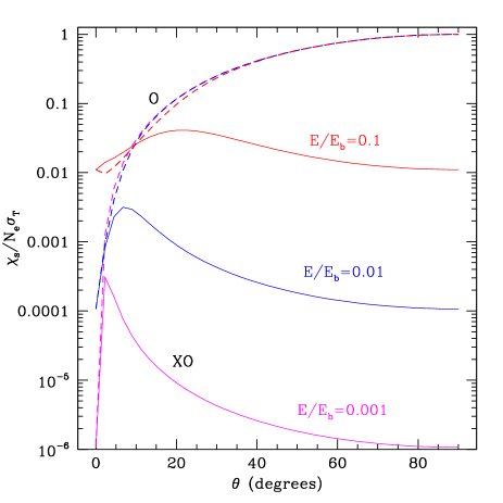
Figure 1: The scattering coefficient $\chi^{s}_{i}$, in units of $N_{e}\sigma_{T}$, for the extraordinary (solid lines) and the ordinary (dashed lines) mode as a function of $\theta$ for $E/E_{b}=0.1,0.01$, and $0.001$.

The magnetic scattering and absorption coefficients have strong dependences on the direction of propagation and photon energy, and the two modes show increasingly different behavior with increasing magnetic field strength. To facilitate the discussion in $\S 4$ and make our results more intuitive, we plot in Figure 1 the scattering coefficients $\chi^{s}_{i}$ as a function of $\theta$ for $E/E_{b}=0.1$, $0.01$, and $0.001$. The solid lines show the extraordinary and the dashed lines show the ordinary-mode opacities. In $\S 4.3$, we will show that the beaming of emerging radiation for different values of $E/E_{b}$ is closely related to the behavior of the opacities shown in Figure 1.

2.3 Vacuum Polarization

In strong magnetic fields, in addition to the response of the plasma electrons, the vacuum polarization effects due to the virtual electron-positron pairs also become significant (Adler 1971; Gnedin et al. 1978; Mészáros & Ventura 1978, 1979) and contribute to the dielectric tensor and the magnetic permeability tensor. Thus, the vacuum polarization alters the polarizations of the normal modes and affects the interaction cross sections in the plasma (see Pavlov & Shibanov 1979; Mészáros & Ventura 1979; Mészáros 1992). The effect of the magnetic vacuum can be quantified by the parameter

$$W=\left(\frac{3\times 10^{28}{\rm cm}^{-3}}{N_{e}}\right)\left(\frac{B}{B_{cr}}\right)^{4}.$$ (1)

which enters the ellipticity parameter $q$ of the normal modes through

$$q=\frac{\sin^{2}\theta}{2\cos\theta}\sqrt{u}\left(1-W\frac{u-1}{u^{2}}\right),$$ (2)

where $u=E_{b}^{2}/E^{2}$. The resulting normal modes of the magnetic vacuum, in the absence of plasma electrons, are linearly polarized at $\theta=0$ and $\theta=\pi/2$, and elliptically polarized at all other angles of propagation. Note that the ellipticity parameter $q$ has a slightly modified form for $B>B_{cr}$ but this does not affect qualitatively the emerging spectrum (Özel & Narayan 2001).

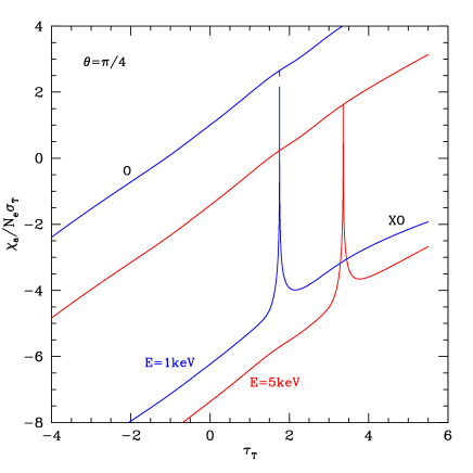
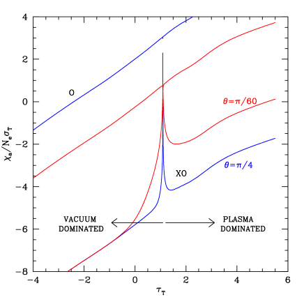
Figure 2: The absorption coefficient $\chi^{a}_{i}$, in units of $N_{e}\sigma_{T}$, of the extraordinary and ordinary modes as a function of density in the atmosphere in the presence of vacuum polarization at two photon energies (top panel) and for two directions of propagation at $E=0.5$ keV (bottom panel).

When both plasma electrons and virtual pairs are present, the normal modes of propagation at very high plasma densities (plasma-dominated region) are different than those at very low plasma densities (vacuum-dominated region) and go through a transition at a critical density where plasma electron and virtual pair contributions identically cancel out (see Fig. 2). At this critical density, a resonance appears at the point where $q$ changes sign and the linear polarizations of the normal modes vanish, leaving the modes purely circularly polarized. (Strictly at the critical frequencies, the orthogonality of the normal modes also vanishes, rendering the normal mode treatment invalid; see Mészáros & Ventura 1979 for a discussion). For $W>4$, the $q=0$ condition can be written as

$$E^{2}=0.5E_{b}^{2}\left[1\pm(1-4/W)^{1/2}\right],$$ (3)

which gives the critical photon energies for each density where this resonance appears. Alternatively, the same equation can be used to determine the critical density at which the resonance occurs for each photon energy $E\leq E_{b}$.

The most important effect of the vacuum resonance is that, for each photon energy, the opacities of the two modes have a close approach or become equal at the critical density depending on the value of $\mu$, with a strong enhancement of both the scattering and absorption coefficients of the extraordinary mode, including the off-diagonal, mode-changing terms of the scattering matrix. Figure 2 shows the opacities with vacuum resonance as a function of $\tau_{T}=\int N_{e}\sigma_{T}dz$ in the atmosphere (see also §3.1). The resonance occurs over a narrow range of densities, which leads to broadband absorption-like features in the spectrum (see §4.3 and also Bulik & Miller 1996). Finally, the eigenmodes of the pure vacuum are similar to those of the electron plasma for most angles $\theta$, but differ significantly at a very small range of angles near $\theta=0$. Therefore, even though an extraordinary-mode photon can convert into an ordinary-mode photon across the resonance through scattering, the definitions of the “extraordinary” and the “ordinary” modes essentially remain the same above and below the resonant density (see also Fig. 2 and Mészáros 1992).

The vacuum resonance has a finite narrow width in photon energy and electron density. For a given photon energy and direction of propagation, the width of the resonance corresponds to a change in $q$, of

$$\Delta q\simeq\frac{\sin^{2}\theta}{2\cos\theta}\frac{E_{b}}{E}\frac{\Delta N}{N},$$ (4)

and occurs over a fractional change in electron density of $\Delta N/N\lesssim 1\%$. We include in our calculations the effects of vacuum polarization through the normal mode ellipticity parameter, as given in Kaminker et al. (1982). However, due to the numerical resolution which prevents us from sampling the change in electron density to the required accuracy even with 400 depth points, we force the resonance to saturate by choosing for $|q|$ a minimum allowed value across the resonance of

$$|q|\geq\xi\frac{\sin^{2}\theta}{2\cos\theta}\frac{E_{b}}{E}\,.$$ (5)

We have experimented with the factor $\xi$ and found that for our resolution, $\xi\sim 1\%$ results in smooth spectra with negligible change in the total and scattering optical depth. This is equivalent to assuming that at a given $\tau_{\rm T}$, the density fluctuates to within $\sim 1\%$.

Our results show that specifically, for $B>10^{14}$ G and at densities $N_{e}\lesssim 10^{27}{\rm cm}^{-3}$, $W\gg 1$ and therefore the temperature profiles of the atmospheres as well as the emerging spectra at energies above 1 keV are significantly modified by vacuum polarization (see §4.1 and 4.3). Already based on Figure 2, one can see that this resonance is expected to attenuate the emerging flux and lead to a heating of the atmosphere at the $1\lesssim\tau_{\rm T}\lesssim 10^{4}$, which corresponds to the density range that includes the critical density for most flux carrying ($0.5-5$ keV) photons.

2.4 Model Atmospheres

We choose as the dimensionless depth variable the Thomson optical depth, $d\tau_{\rm T}=N_{e}\sigma_{T}dz$, and define a logarithmic grid of typically 100-400 equally spaced points between $10^{-5}$ and $10^{5}$. In terms of this stratification parameter, the equation of transfer in the two modes can be written as

$$y_{G}\mu\frac{dI_{E}^{i}}{d\tau_{\rm T}} = \chi^{a}_{i}\left[I_{E}^{i}-\frac{B_{E}(T)}{2}\right]+\chi^{s}_{i}I_{E}^{i}$$ (6)

$$-\sum_{j}\int\chi^{s}_{ji}(\mu,\mu^{\prime})I_{E}^{j}(\mu^{\prime})d\mu^{\prime}\;,$$

where $B_{E}(T)$ is the Planck function, $\chi^{a}_{i}$ and $\chi^{s}_{i}$ denote the total absorption and scattering coefficients in Thomson units ($N_{e}\sigma_{T}$), respectively, and $\chi^{s}_{ij}(\mu,\mu^{\prime})$ is the angle- and polarization-dependent scattering coefficient. The parameter $y_{\rm G}$ takes into account the effects of general relativity and is defined as

$$y_{\rm G}\equiv\sqrt{1-\frac{2GM_{\rm NS}}{R_{\rm NS}c^{2}}}\;,$$ (7)

where $G$ is the gravitational constant, $c$ is the speed of light, and $M_{\rm NS}$ and $R_{\rm NS}$ are the neutron-star mass and radius, respectively. In the following calculations, we set $M_{\rm NS}=1.4M_{\odot}$ and $R_{\rm NS}=10^{6}$ cm. Since there are no sources or sinks of heat, the atmospheres are in radiative equilibrium, specified by

$$H_{\rm eff}=\frac{1}{2}\sum_{i}\int\int I_{E}^{i}(\mu)\mu d\mu dE\equiv\frac{1}{4\pi}\sigma T_{\rm eff}^{4}\;,$$ (8)

where $4\pi H_{\rm eff}$ is the (constant) radiation flux and $T_{\rm eff}$ is the effective temperature.

The momentum balance in the atmosphere is specified by the hydrostatic equilibrium condition

$$\frac{dP}{d\tau_{\rm T}}=\frac{g\rho}{y_{G}^{2}N_{e}\sigma_{T}}\;,$$ (9)

where $P$ is the pressure, $\rho$ is the density, and $g=GM_{\rm NS}/R_{\rm NS}^{2}$. This system of equations describe the state of the plasma and can be closed assuming an equation of state, which to first approximation can be taken to be that of an ideal gas (see §2.1),

$$P=2N_{e}kT\;,$$ (10)

where the factor of 2 is valid for completely ionized H gas. Equations (9) and (10) can be easily integrated from the surface inwards, to give

$$N_{\rm e}=\frac{gm_{\rm p}\tau_{\rm T}}{2y_{G}^{2}\sigma_{T}kT}\;,$$ (11)

where $m_{\rm p}$ is the proton mass. The temperature and density profile of the atmosphere is obtained by solving these equations coupled with the radiation field. The iterative method of solution for this set of equations is described in the next section.

3 The Method

We compute the radiative equilibrium model atmospheres using an iteration procedure that involves the solution of the equation of radiative transfer through a Feautrier method and makes use of the linearized moment equations to determine the temperature profile.

3.1 Radiative Transfer

We follow a modified Feautrier method (Mihalas 1978) for the solution of the radiative transfer problem. This method allows for a complete, non-iterative solution (of the transfer equation), including the effects of angle-dependent scattering and absorption cross sections. Because we need only to consider conservative scattering, we solve the transfer equation at each photon energy separately.

We begin by writing the equation of radiative transfer for the two modes as

$$y_{\rm G}\mu\frac{\partial I_{E}^{i}}{\partial\tau_{i}}=I_{E}^{i}-S^{i}\;,$$ (12)

where

$$d\tau^{i}\equiv(\chi^{a}_{i}+\chi^{s}_{i})d\tau_{\rm T}$$ (13)

is the total optical depth at each mode and we have defined the energy-dependent source function as

$$S^{i}\equiv\frac{\chi^{a}_{i}}{\chi^{a}_{i}+\chi^{s}_{i}}\frac{B}{2}+\frac{1}{\chi^{a}_{i}+\chi^{s}_{i}}\sum_{j}\int\chi^{s}_{ij}(\mu,\mu^{\prime})I_{E}^{j}(\mu^{\prime})d\mu^{\prime}\;.$$ (14)

In the following equations we drop the energy subscript and explicitly specify any energy-integrated quantities.

We define the Feautrier variables

$$u^{i}\equiv\frac{I_{E}^{i+}+I_{E}^{i-}}{2}$$ (15)

and

$$v^{i}\equiv\frac{I_{E}^{i+}-I_{E}^{i-}}{2}.$$ (16)

We then write the transfer equation [12] as two first-order equations

$$y_{\rm G}\mu\frac{\partial u^{i}}{\partial\tau_{i}}=v^{i}$$ (17)

and

$$y_{\rm G}\mu\frac{\partial v^{i}}{\partial\tau_{i}}=u^{i}-S^{i}\;,$$ (18)

which can be combined to give one second-order equation for the variable $u$

$$y_{\rm G}^{2}\mu^{2}\frac{\partial^{2}u^{i}}{{\partial\tau_{i}}^{2}}=u^{i}-S^{i}\;.$$ (19)

Note here that, unlike the usual Feautrier equations, in which the source function involves an integral over only photon momentum, the source function in equation [19] involves also a summation over the photon polarization mode, introducing a coupling between the two equations. However, the off-diagonal (mode-changing) elements of the scattering coefficients, $\chi^{s}_{ij}(\mu,\mu^{\prime})$ ($i\neq j$), are in general much smaller than the diagonal elements away from the cyclotron resonance, and can be treated as a perturbation. Making use of this fact, we solve iteratively the Feautrier equation for each mode separately, assuming that the coupling terms are known from the previous iteration, until the local specific intensity converges to one part in $\sim 10^{9}$.

The transfer problem is highly coupled in the three variables $\tau_{\rm T},E$, and $\mu$ so that choosing a discretization grid is one of the most delicate parts of the calculation. We discretize the second-order equation (19) on the predefined grid over the variable $\tau_{\rm T}$ (and not over $\tau_{i}$, which depends on $\mu$ and $E$), according to Mihalas (1978; eq. [6.26]-[6.30]). We use

$$\Delta\tau_{i,d\pm 1/2}\equiv\frac{1}{2}(\chi^{\rm tot}_{i,d}+\chi^{\rm tot}_{i,d\pm 1})|\tau_{\rm T,d}-\tau_{\rm T,d\pm 1}|$$ (20)

where $\chi^{\rm tot}_{i}\equiv\chi^{a}_{i}+\chi^{s}_{i}$. The chosen range for $\tau_{\rm T}$ (see §2.3) corresponds to a range in the optical depth in the extraordinary mode ($\tau_{1}$) of $0.0001-10$ (depending on the photon energy and direction of propagation) and in the ordinary mode ($\tau_{2}$) of $0.001-10^{4}$. We chose this range so that all photon energies of interest turn optically thick in the deep interior and decouple from the atmosphere at small optical depths.

Because of the very strong dependence of magnetic opacities on angle near $\mu\simeq 1$, we choose a logarithmic grid (typically of 30–40 points) in the quantity $1-\mu$, with $\log(1-\mu)=-5\rightarrow 0$. We also choose a logarithmic grid (typically of 40 points) in photon energy, with $\log E=-3\rightarrow 1.5$. This range spans the photon energies that carry most of the radiative flux for the effective temperatures ($\sim 0.1-0.5$ keV) of our atmosphere. Note that the highest number of points in depth, photon energy, and angle are required in those calculations where the vacuum polarization effects are significant.

Finally, we follow the procedure described in Mihalas (1978) to evaluate and invert the Feautrier matrices.

3.2 Temperature Correction Scheme

We start with an initial guess for the temperature profile

$$T=\left[\frac{3}{4}\left(\tau_{\rm R}+\frac{2}{3}\right)\right]^{1/4}T_{\rm eff}\,$$ (21)

where $\tau_{\rm R}$ is the optical depth that corresponds to the Rosseland mean opacity $\chi_{\rm R}$, defined as (Pavlov et al. 1992)

$$\frac{1}{\chi_{\rm R}}=\frac{3\pi}{8\sigma T^{3}}\int_{-1}^{1}d\mu\int dE\left[\frac{1}{\chi^{\rm tot}_{1}}+\frac{1}{\chi^{\rm tot}_{2}}\right]\frac{\partial B_{E}(T)}{\partial T}$$ (22)

for two polarization modes and calculate the corresponding density $N_{e}(\tau_{\rm T})$ using equation (11). We then proceed by calculating the magnetic opacities with this guess temperature profile on our predetermined grid and solve the radiative transfer problem.

In order to determine the temperature profile of the model neutron star atmosphere in radiative equilibrium, we use an iterative temperature correction scheme similar to the Unsöld-Lucy algorithm, which utilizes the energy-integrated moment equations in order to obtain a linear perturbation equation for $\Delta T(\tau_{\rm T})$ (see Mihalas 1978). However, despite the similarity of the approach, the scheme we describe here differs from the Unsöld-Lucy scheme in two important respects:

(i) We do not make any assumptions about the angular distribution of the radiation field, which is the case when the Eddington approximation is used. Instead, we calculate at each iteration the Eddington factor $f=K/J$ as a function of $\tau_{\rm T}$, as well as the ratio $K/H$ at the boundary $\tau_{\rm T}=0$, where $J,H$, and $K$ denote the zeroth, first, and second moments of the specific intensity, respectively. This takes into account the deviations from anisotropy in the radiation field which are likely to be present in strongly magnetized plasmas.

(ii) We include first-order corrections in all temperature-dependent quantities due to a temperature change $\Delta T$, except for the radiation intensity itself. This is in contrast to the assumption in the Unsöld-Lucy procedure, that only the local blackbody source function changes with temperature.

With these modifications, the correction scheme proceeds as follows. We start with the energy-integrated zeroth and first moment equations

$$y_{G}\frac{\partial H}{\partial\tau_{\rm T}}=\chi_{J}J-\chi_{P}B$$ (23)

and

$$y_{G}\frac{\partial K}{\partial\tau_{\rm T}}=\chi_{F}H\;,$$ (24)

where $\chi_{J},\chi_{P}$, and $\chi_{F}$ are similar to (Mihalas 1978) the absorption mean, Planck mean, and flux mean opacities, respectively, appropriately defined for a magnetized atmosphere. In particular

$$\chi_{P}\equiv\frac{\pi}{2}\left[\frac{\int d\mu\int dEB_{E}(T)(\chi^{a}_{1}+\chi^{a}_{2})/2}{\sigma_{T}T_{\rm eff}^{4}}\right]\;,$$ (25)

$$\chi_{J}\equiv\frac{\int d\mu\int dE(\chi^{a}_{1}u^{1}+\chi^{a}_{2}u^{2})}{\int d\mu\int dE(u^{1}+u^{2})}\;,$$ (26)

and

$$\chi_{F}\equiv\frac{\int d\mu\int dE\mu(\chi^{\rm tot}_{1}v^{1}+\chi^{\rm tot}_{2}v^{2})}{\int d\mu\int dE\mu(v^{1}+v^{2})}\;.$$ (27)

In the above definitions, we implicitly assume that the moments and the mean opacities depend on $\tau_{\rm T}$ and omit any explicit references.

Integrating equation (24) and substituting into equation (23) by making use of the Eddington factors, which are known from the current iteration, yields

$$\chi_{P}B=\chi_{J}\left(\frac{J}{K}\right)\left[\left(\frac{K}{H}\right)_{0}H(0)+\frac{1}{y_{G}}\int\chi_{F}(\tau_{\rm T}^{\prime})H(\tau_{\rm T}^{\prime})d\tau_{\rm T}^{\prime}\right]-y_{G}\left(\frac{dH}{d\tau_{\rm T}}\right),$$ (28)

where the subscript 0 corresponds to the outer boundary. We assume that the constant flux solution can be obtained by making a small correction $\Delta T(\tau_{\rm T})$ everywhere in the atmosphere and allow for the local black body and the mean opacities to vary linearly with $\Delta T$, which gives $\Delta B(\tau_{\rm T})=(\partial B/\partial T)\Delta T\equiv B^{\prime}(\tau_{\rm T})\Delta T,\Delta\chi_{P}=\chi_{P}^{\prime}\Delta T$, and similarly for the other mean opacities. Note that all the derivatives are computed at the $\tau_{\rm T}$ grid points. Now proceeding as in the Unsöld-Lucy scheme, we note that in the desired radiative equilibrium solution, the term $\partial H/\partial\tau_{\rm T}$ vanishes and the radiation flux becomes $H(\tau_{\rm T})=H_{\rm eff}=\frac{1}{4\pi}\sigma_{T}T_{\rm eff}^{4}$. Thus, subtracting the current equation from the desired constant flux solution and solving for $\Delta T$ we obtain

$$\Delta T(\tau_{\rm T})=\frac{\chi_{J}(J/K)_{\tau}\left[(K/H)_{0}\Delta H(0)+I_{1}\right]+y_{G}({\rm d}H/{\rm d}\tau)_{\tau}}{\chi_{P}^{\prime}B+\chi_{P}B^{\prime}-\chi_{J}^{\prime}(J/K)_{\tau}\left(K/H)_{0}H_{\rm eff}+I_{2}\right]},$$ (29)

where

$$I_{1}=\frac{1}{y_{G}}\int_{0}^{\tau}[\chi_{F}(\tau_{\rm T}^{\prime})\Delta H(\tau_{\rm T}^{\prime})+\chi_{F}^{\prime}(\tau_{\rm T}^{\prime})\Delta T(\tau_{\rm T}^{\prime})H_{\rm eff}]\rm{d}\tau_{\rm T}^{\prime}\,,$$ (30)

$$I_{2}=\frac{1}{y_{G}}\int_{0}^{\tau}[\chi_{F}(\tau_{\rm T}^{\prime})+\chi_{F}^{\prime}(\tau_{\rm T}^{\prime})\Delta T(\tau_{\rm T}^{\prime})]H_{\rm eff}\rm{d}\tau_{\rm T}^{\prime}\,,$$ (31)

and $\Delta H(\tau_{\rm T})=H_{\rm eff}-H(\tau_{\rm T})$ refers to the deviation of the current solution from the constant flux solution at any depth in the atmosphere. To quantify this deviation, we define the error $e=[H_{\rm eff}-H(\tau_{\rm T})]/H_{\rm eff}$ and quote the convergence of the obtained solutions in terms of this quantity.

Due to the assumption of linear changes in various quantities in response to a temperature correction $\Delta T$, care must be taken when applying large temperature corrections which may violate this assumption. To this end, we have introduced a damping factor to control the actual applied change everywhere in the atmosphere. We experimented with damping factors that depend on the magnitude of $\Delta T(\tau_{\rm T})$ and found that reducing the $\Delta T$ obtained from the above scheme typically by $0.3-0.5$, even though somewhat slowing down the convergence rate, results in a marked increase in the stability of the algorithm. With this method, we achieve flux convergence down to a maximum error of $e\approx 5\%$ in $O(10)$ iterations, improving it to everywhere better than $1\%$ in $O(100)$ iterations.

Comparing the scheme described here with the Unsöld-Lucy algorithm, we note that the correction in temperature at any point in the atmosphere, $\Delta T(\tau_{\rm T})$, depends not only on the errors in the flux everywhere in the atmosphere outward of that location (as in the Unsöld-Lucy scheme) but also on the temperature corrections applied at all other points. This allows for stronger coupling between all points in the atmosphere and leads to a more uniform convergence. At the same time, convergence is much more stable, and artificial temperature inversions that commonly arise when applying the Unsöld-Lucy scheme to magnetized atmospheres are not present.

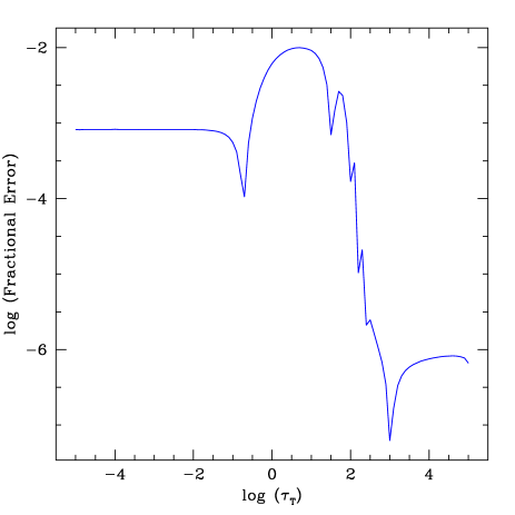
Figure 3: The deviation from a constant flux solution throughout the neutron star atmosphere. See the text for the definition of the flux error. The parameters are $B=10^{14}$ G and $T_{\rm eff}=0.3$ keV, chosen as a typical example.

Finally, note that any temperature correction scheme that allows for a change in the intensity field with temperature, such as the complete linearization schemes (Mihalas 1978), couples the different photon energies in the solution of the radiative transfer problem and thus requires $O(N_{E}^{3})$ operations in the Feautrier method, where $N_{E}$ is the number of grid points in photon energy. As a result, the total computational time required for solving the radiative transfer problem scales as $O(M^{3}N_{E}^{3})$, with M denoting the number of points on the $\mu=\cos(\theta)$ grid, thus limiting the computational resolution in one or both of these variables. In such a highly angle- and photon energy-dependent problem as the magnetized radiative transfer, we have opted to work with the largest number of grid points in a feasible amount of computational time and therefore chose to work with the temperature correction scheme discussed above.

We apply the method described above to construct magnetized, radiative equilibrium atmospheres with a flux $H(\tau)$ that is converged to within $1\%$ of $H_{\rm eff}$, everywhere in the atmosphere. Figure 3 shows the magnitude of typical errors that result from such a calculation. Throughout most of the atmosphere, the fractional error is $e\ll 1\%$, reaching $10^{-8}$ in the deep interior. We have found that the slowest convergence, and thus the maximum error, occurs typically in the transition region, where the photons carrying the largest flux become optically thin; we will discuss this transition region below. We also note that the convergence criterion of $1\%$ does not arise from an intrinsic limitation of the algorithms, but is chosen in view of the required computational time.

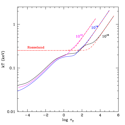
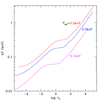
Figure 4: (Top panel) The temperature profiles of three model atmospheres plotted against $\tau_{\rm T}$, at $B=10^{13},10^{14}$, and $10^{15}$ G, with $T_{\rm eff}=0.3$ keV. The dashed lines correspond to the temperature profiles calculated using the Rosseland mean opacities. (Bottom panel) The variation of the temperature profiles with $T_{\rm eff}$ for magnetic field strength fixed at $B=10^{14}$ G.

4 Results

We have applied the method described above to construct magnetized, radiative equilibrium atmospheres of neutron stars with a range of magnetic field strengths ($10^{13}$ G$\leq B\leq 10^{15}$ G) and effective temperatures ($0.1$ keV$<T_{\rm eff}<0.5$ keV). We show below the resulting temperature profiles, spectra, and beaming of emerging radiation and identify the effects of magnetic field strength, effective temperature, scattering, and vacuum polarization on each of these properties.

4.1 Temperature Profiles

Figure 4 shows the temperature profiles for three model atmospheres with different magnetic field strengths, at $T_{\rm eff}=0.3$ keV (top panel). These profiles have distinct features arising from the strong angle- and energy-dependence of the magnetic opacities and the presence of two polarization modes and are significantly different from the temperature profile of a grey atmosphere (see, e.g., Mihalas 1978) and from an atmosphere calculated using Rosseland mean opacities (dashed lines). In particular, at low optical depths, the temperature is determined primarily by the ordinary-mode opacities, which depend very weakly on the magnetic field strength, for most directions of propagation. Therefore, the temperature profiles in this region are similar in all three model atmospheres (but see below for the role of vacuum polarization in this region). This is also the reason why the Rosseland mean opacities, which are dominated by the small opacity (extraordinary) mode, fail to describe the temperature of the outer atmosphere correctly. At the limit of high optical depth, the diffusion limit is reached and the temperatures calculated using the Rosseland mean opacities provide an accurate description of the atmospheres. At these high optical depths, it is the extraordinary-mode opacities, which are low and depend strongly on the field strength, that determine exclusively the temperature profiles. As a result, with increasing magnetic-field strength, the same plasma temperature is reached deeper in the atmosphere.

The presence of multiple plateaus in the temperature profiles correspond to optically thick/thin transitions of photons with different energies, directions of propagation, and polarizations. Specifically, the plateaus at $\tau_{\rm T}\sim 10^{0}-10^{2}$ arise from such transitions of extraordinary-mode photons that carry most of the flux, while the plateaus at $\tau_{\rm T}\lesssim 10^{-4}$ are the result of such transitions for the ordinary-mode photons with low energies or large angles of propagation.

One other significant difference between the profiles of Figure 4 and the temperature profile of a grey/Rosseland atmosphere is the relation between the effective temperature and the plasma temperature $T_{0}$ at the outer boundary. For a grey atmosphere, $T_{0}\simeq 0.8T_{\rm eff}$, whereas for the calculations shown in Figure 4, $T_{0}\simeq 0.1T_{\rm eff}$. The same conclusion is reached by Shibanov et al. (1992), but the agreement is only qualitative due to the insufficiency of the diffusion approximation employed in that work in capturing the details of the temperature profiles.

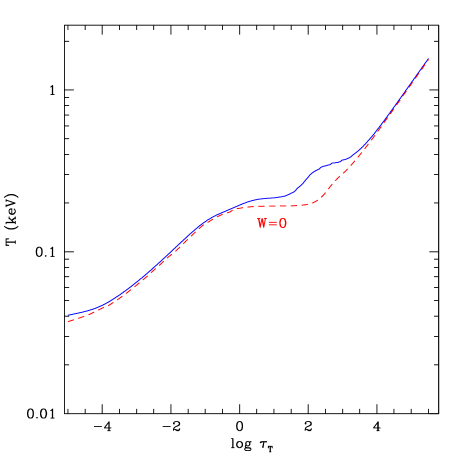
Figure 5: The difference in the temperature profiles when the vacuum effects are included (solid line) and neglected (dashed line) at $B=10^{15}$ G.

The temperature profiles of model atmospheres with different effective temperatures, as shown in Figure 4 (bottom panel), have the same qualitative characteristics, but show an overall displacement. In addition, the plateaus occur further out in the atmosphere with decreasing effective temperature, as the absorption cross sections increase with decreasing temperature, moving the optically thick/thin transitions to smaller column densities.

At $B\sim 10^{15}$ G, the temperature profiles are significantly affected by the vacuum polarization resonance. To demonstrate the vacuum resonance effects on the temperature profile, we show in Figure 5 the results of two calculations at $B=10^{15}$ G and $T_{\rm eff}=0.3$ keV, where we include (solid lines) or neglect (dashed-lines) the vacuum polarization contribution to the magnetic opacities. The temperature is higher for a range of optical depths $1\lesssim\tau_{\rm T}\lesssim 10^{3}$ in the case where the vacuum polarization contribution to the opacities are included. Such an increase in temperature is typical of radiative equilibrium atmospheres with a resonant layer at low densities for reasons discussed below.

The net effect of the vacuum contribution to the magnetic opacities is to increase the extraordinary-mode opacity for a narrow, photon energy-dependent range of densities in the atmosphere (see §2.2 and Fig. 2). For $B\sim 10^{15}$ G, this resonance appears at $1\lesssim\tau_{\rm T}\lesssim 10^{3}$. Because this range lies within the photosphere where the extraordinary mode photons of $0.5-10$ keV have decoupled from the atmosphere, the resonance leads to an attenuation of the flux at these photon energies, which appears as a broad-band absorption feature in the spectrum (see §4.3). At the same time, the additional absorption of radiation heats the atmosphere, thus leading to an increase in the temperature at this range of column densities (Fig. 5). This in turn increases the emission at these column depths and contributes to the flux at lower photon energies. We note that it is also possible to understand these results in terms of the radiative equilibrium condition in the atmosphere. In the presence of resonant “layers” of high opacity, the overall temperature in the atmosphere has to increase in order for the energy-integrated flux to be constant throughout the atmosphere, for a given effective temperature. This change in the temperature profile results in a corresponding change in the entire emerging spectrum at the highest magnetic field strengths, as we will show in the next section.

4.2 Spectra of Emerging Radiation

In Figure 6, we show the spectra emerging from neutron star atmospheres with different magnetic field strengths and effective temperatures. In the top panel, the flux is decomposed into the relative contributions of the two polarization modes while in the bottom panel the total flux is shown. Note that the fluxes shown are in accordance with the definition of $H$ given in $\S 2.3$ and the total radiative flux is given by $4\pi H$; the subscript $E$ as usual denotes the energy dependence. The detailed features of the spectra result mainly from the combined effects of the temperature profile, the scattering between polarization modes, and the polarization of the magnetic vacuum, which we discuss below. The magnetic field strength enters all of these factors and thus affects the emerging spectra in multiple ways.

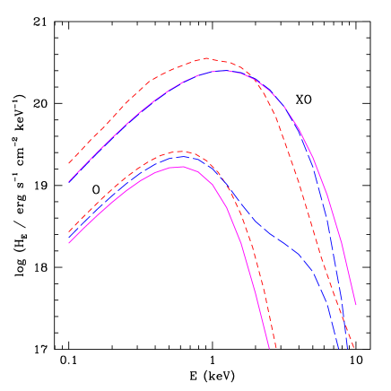
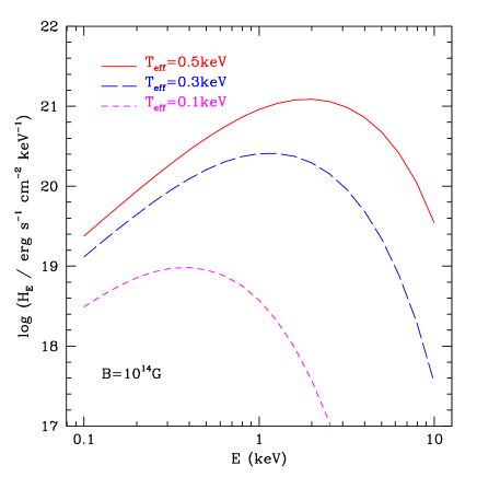
Figure 6: (top panel) Spectra of emerging radiation at $B=10^{13}$ G (long-dashed line), $10^{14}$ G (solid line), and $10^{15}$ G (short-dashed line) for $T_{\rm eff}=0.3$ keV. The flux in the two modes are shown separately; the labels ‘O’ and ‘XO’ refer to the ordinary and the extraordinary modes, respectively. (bottom panel) Same as above, but for a fixed magnetic field strength of $B=10^{14}$ G and for $T_{\rm eff}=0.1$ keV (short-dashed line), $0.3$ keV (long-dashed line) and $0.5$ keV (solid line). Here, the contributions of the two modes are added and the total flux is plotted. The radiative flux is equal to $4\pi H_{E}$.

Two results hold in all cases: (i) the extraordinary mode carries most of the radiative flux and (ii) the spectra are not Planckian, showing various amounts and shapes of hard excess. The first result arises from the fact that the opacity of the extraordinary mode is significantly smaller and hence it decouples from the plasma at greater depths, where the temperature is higher (Fig. 6). The second result is primarily, but not exclusively, due to a similar reason: as shown previously (e.g., Shibanov et al. 1992; Rajagopal & Romani 1997), the high-energy photons originate deeper in the atmosphere due to their smaller interaction cross section and hence the emerging spectra are bluer than the blackbody spectrum at the effective temperature. The spectral hardening because of the energy-dependence of the opacities is less pronounced in the case of high magnetic fields than non-magnetic neutron star atmospheres because the dependence of the magnetic free-free opacity on photon energy $(K\propto E^{-1})$ is weaker than that of the non-magnetic one $(K\propto E^{-3})$ (see also Zane, Turolla, & Treves 2000). However, it is important to note that in the case of ultrastrong magnetic fields, different photospheres for different energy photons is not the only origin of hard excess in the spectra and the hard tails do not decrease monotonically with increasing magnetic field strength. Instead, the spectral shape is determined by two other effects. First, as we will show in §4.3, the broad-band absorption due to vacuum resonance changes the spectral shape to reduce the color temperature $T_{c}$ of the best-fit blackbody but gives rise to a pronounced power-law tail. This is because of the energy- and density-dependence of the vacuum resonance as shown in Figure 2. Second, scattering of photons from the extraordinary mode to the ordinary mode, especially enhanced in the presence of vacuum polarization resonance, reduces the spectral hardening. We also show this below.

As the bottom panel in Figure 6 shows, the effective temperature controls the total emerging flux, as well as the peak and broadness of the spectrum. Although the scaling of the total flux with $T_{\rm eff}$ is straightforward, the flux at each photon energy does not scale in the same way. This is because the temperature profiles corresponding to different $T_{\rm eff}$ differ by more than a simple displacement (see §4.1). Specifically, the outer layers can be significantly hotter for higher effective temperatures, giving rise to more flux at low photon energies. For a similar reason, the spectra emerging from atmospheres with higher $T_{\rm eff}$ are more peaked, with an increasing fraction of the total flux emerging around the peak photon energy.

The effects of scattering between different polarization modes are strongest at the lowest magnetic-field strengths, because, for a given photon energy, the off-diagonal element of the scattering coefficient from the extraordinary mode to the ordinary mode increases with decreasing field strength. On the other hand, the effects of the polarization of the magnetic vacuum are strongest at the highest field strengths, as discussed in §2.2. In order to disentangle these two effects, we discuss the lowest ($10^{13}$ G) and the highest ($10^{15}$ G) magnetic field strengths in more detail, thus isolating each effect.

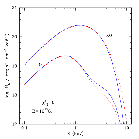
Figure 7: The spectra emerging from a model atmosphere with $T_{\rm eff}=0.3$ keV and $B=10^{13}$ G, when scattering between different polarization modes is included (solid line) or neglected (dashed line).

We use the temperature profile of the model atmosphere that corresponds to $B=10^{13}$ G and $T_{\rm eff}=0.3$ keV and calculate the emerging spectra, including or neglecting the scattering between polarization modes. As can be seen in Figure 7, the scattering between modes increases the flux of the ordinary mode at high energies. This occurs because the off-diagonal elements of the scattering coefficients increase, when $E$ approaches $E_{\rm b}$. An observable result of this cross-mode scattering is a small suppression of the hard excess at $B\approx 10^{13}$ G. The discussion of the vacuum polarization effects which are strong at $B\sim 10^{15}$ G are presented in the next section.

4.3 Effects of Vacuum Polarization on the Spectrum

Taking into account the contribution of vacuum polarization to the magnetic opacities leads to significant modification in the spectrum of radiation emerging from the neutron star atmosphere. To demonstrate the effects of vacuum resonance, we show in Figure 8 two model spectra where include (solid line) or neglect (dashed line) the vacuum contribution to the scattering and absorption cross sections, using model atmospheres that corresponds to $B=10^{15}$ G and $T_{\rm eff}=0.3$ keV. The result is a drastic change in the overall spectral shape: an increase of the flux at $E\lesssim 2$ keV, an attenuation of the flux at $E\gtrsim 2$ keV and the emergence of a hard spectral tail at $E\gtrsim 3$ keV due to broadband absorption across the vacuum resonance.

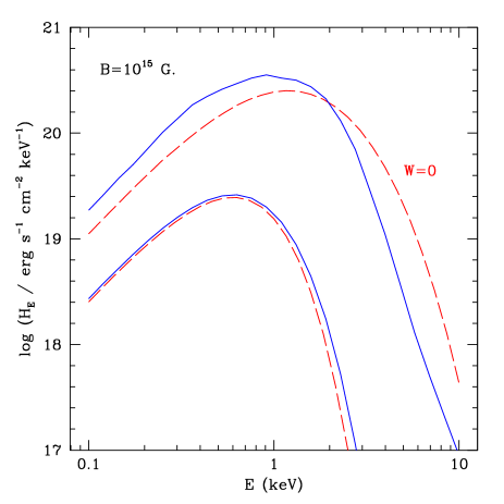
Figure 8: The spectra emerging from a model atmosphere with $T_{\rm eff}=0.3$ keV and $B=10^{15}$ G, when the effects of vacuum polarization are included (solid lines) or neglected (dashed lines).

As Figure 2 shows, the main effect of the contribution of the vacuum polarization to the magnetic opacities for most angles of photon propagation is the emergence of a resonance at a photon-energy dependent critical density in the plasma. When the effects of vacuum polarization are included, at each photon energy, the opacity of the extraordinary mode becomes comparable to that of the ordinary mode and the scattering from the extraordinary mode into the ordinary mode is enhanced for a narrow range of densities. This rapid increase in opacity of the extraordinary mode photons typically occurs at low densities further out in the atmosphere (see Fig. 2), and thus at a density where these photons have already decoupled from the atmosphere. Therefore, the reduction in the flux arises from the fact that going outward in the atmosphere, the essentially free-streaming extraordinary mode photons encounter a resonance and either change polarization mode or are absorbed over a narrow range of $\tau_{T}$. In the latter case, they decouple again outside the resonant layer and stream outward. Note that in the absence of temperature adjustments in the atmosphere, flux in the extraordinary mode at nearly all photon energies would suffer such a reduction. On the other hand, at the densities where the vacuum effects become important, the ordinary mode is mostly optically thick and the reduction of the ordinary-mode opacity due to vacuum contribution is minimal. As a result, the primary effect of vacuum polarization is an attenuation of the flux carried by the extraordinary mode at high photon energies.

The radiative equilibrium condition introduces an additional effect and a further modification of the emerging spectrum. This is because the atmosphere adjusts to the increase in opacity, and the corresponding reduction in the flux, by an overall increase in the temperature in the resonant layers (see §4.1 and Fig. 5). This can also be understood as a heating of the atmosphere due to resonant absorption. This in turn leads to an increase of the flux carried by the low-energy photons (so that the energy-integrated flux is constant) and therefore to an overall shift of the spectrum towards lower energies and a further distortion away from a Planckian spectrum.

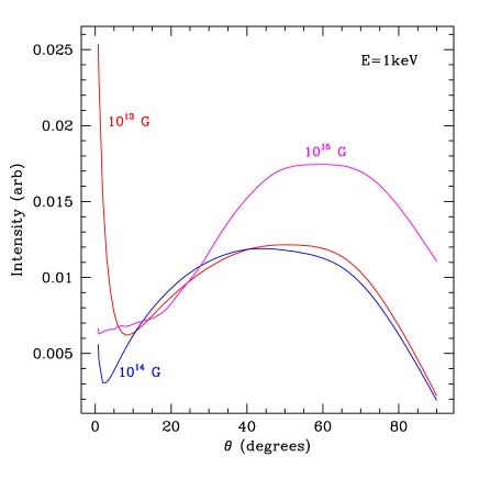
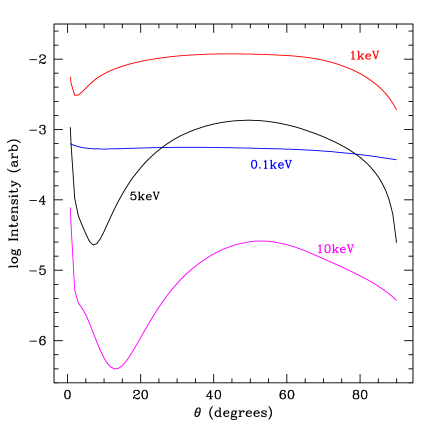
Figure 9: (top panel) Angle dependence of emerging intensity for $T_{\rm eff}=0.3$ keV at $B=10^{13}$G (short-dashed line), $B=10^{14}$ G (long-dashed line), $B=10^{15}$ G (solid line). (bottom panel) Same as above, with $B=10^{14}$ G and $E=0.1$ keV, 1 keV, 5 keV and 10 keV.

4.4 The Beaming of Emerging Radiation

Finally, we discuss the angular pattern of the radiation emerging from the different model atmospheres. In Figure 9 (top panel), we show the beaming of radiation at a photon energy of 1 keV and for three different magnetic-field strengths, while in the bottom panel, we show the beaming of radiation emerging from a model atmosphere with $B=10^{14}$ G, at three different photon energies. Note that the emerging intensity in the ordinary and extraordinary modes are added together in these figures.

Both figures show that the radiation pattern consists of two components: a narrow pencil beam at small angles ($\lesssim 5^{\circ}$) and a broader fan beam at intermediate angles ($\sim 20-60^{\circ}$). This pattern is a direct consequence of the angular dependence of the cross sections in the two modes (see Fig. 1), combined with the temperature profiles in the atmospheres (Fig. 4). In particular, the extraordinary mode contributes to both the pencil and the fan beams, because its opacity is peaked at an angle away from $\theta=0$, decreasing towards both smaller and larger angles. On the other hand, the ordinary mode contributes (roughly equally as the extraordinary mode) to the narrow pencil beam of the pattern, because its opacity decreases significantly at small angles. Therefore while not contributing significantly to the total flux (see §4.2), the ordinary mode plays an important role in determining the beaming pattern with its large specific intensity near $\theta=0$.

The angular dependence of the magnetic cross sections, and hence the beaming of radiation, depend both on photon energy and on magnetic field strength, through the ratio $E/E_{\rm b}$. As Figure 9 shows, at photon energies much smaller than the electron cyclotron energy, the pencil beam is constrained to increasingly smaller angles, $\sin\theta\leq(E/E_{\rm b})^{1/2}$ while the fan beam becomes more prominent, resulting in a flatter radiation pattern. Therefore, for a given magnetic field, the emerging radiation is more strongly and radially beamed at high photon energies, and for a given photon energy the radiation is more beamed at lower magnetic field strengths. Note that with increasing field strength or decreasing photon energy, the peak value of the pencil beam may in fact increase; however the total flux in the pencil beam decreases, thus making it less prominent. Numerically, the pencil beam in such cases, constrained to $\theta\lesssim 0.1^{\circ}$, becomes hard to resolve and has minimal observational consequences.

In addition, at $B\simeq 10^{15}$ G, vacuum polarization affects the beam shape at photon energies $E\gtrsim 1$ keV. Specifically, the scattering cross sections are enhanced due to the vacuum contribution, redistributing the photons between the two polarization modes and different angles of propagation more efficiently. This results in a beam shape with a broader pencil component and a broader plateau between the pencil and fan beams than that of the $B=10^{14}$ G case (Fig. 8) and the case when the vacuum contribution is ignored.

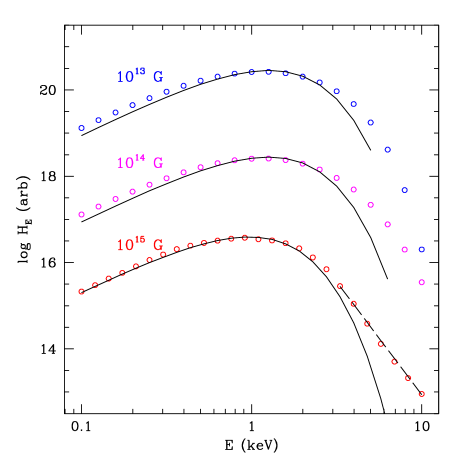
Figure 10: The spectra (open circles) emerging from neutron staratmospheres with $T_{\rm eff}=0.3$ keV and different magnetic field strengths, along with the best-fit black body spectra in the photon energy range $0.5-10$ keV (solid lines). At $10^{15}$ G, the dashed lines represent the best-fit power-law spectral tail at high photon energies. All spectra are displaced vertically for clarity.

5 Discussion and Conclusions

We have constructed model atmospheres for strongly magnetic neutron stars in radiative equilibrium. We have considered the complete angle, polarization and energy dependence of the magnetic free-free absorption and scattering processes, taking into account the effects of polarizability of the magnetic vacuum. We find that the resulting spectra are broader and bluer than the black body spectrum at the effective temperature, and depend on the magnetic field strength.

Figure 10 shows the dependence of the emerging spectra on magnetic field strength for $T_{\rm eff}=0.3$ keV along with the best-fit black body spectra in the photon energy range $0.5-10$ keV, displaced vertically for clarity. In determining the best fit blackbody and the color temperature $T_{\rm c}$, we fit the peak of the spectra and allow for a hard excess, either in the form of a power-law tail or a broad excess. For $B\lesssim 10^{14}$ G, the spectra have distorted Planckian shapes and are generally broader than a black body. Therefore, when fitted with black body shapes, the best-fit (color) temperatures, $T_{\rm c}$ depend on the range of photon energies used (see Table 1). Typically, for these magnetic fields, $T_{\rm c}/T_{\rm eff}\simeq 1.5-1.8$.

At $B>10^{14}$ G, the spectra are significantly modified by the vacuum polarization effects and are in general well-described by a black-body shape at low energies with a high energy power-law tail. The corresponding color temperatures are smaller (see Table 1), with $T_{\rm c}/T_{\rm eff}\simeq 1.2$ at $B=10^{15}$ G. For this magnetic field strength, the power-law tail has an energy index of $-4$.

At all magnetic field strengths, the angular dependence has two maxima: a narrow (pencil) beam at small angles ($\lesssim 5^{\circ}$) with respect to the normal and a broad maximum (fan beam) at intermediate angles ($\sim 20-60^{\circ}$). The relative importance and the opening angle of the radial beam decreases strongly with increasing magnetic field strength and decreasing photon energy (see §4.3). As a result, the emerging radiation from a thermally-emitting neutron star has a prominent radial peak only at relatively low magnetic field strengths ($B\sim 10^{13}$ G) and at high photon energies ($E\gtrsim 1$ keV) within the range of $B$ and $E$ values considered here.

Our results have significant implications for models of thermally emitting neutron stars with strong magnetic fields, and specifically for magnetar models of SGRs and AXPs. First, the observed power-law spectral tails at high photon energies need not arise from a non-thermal (possibly magnetospheric) emission mechanism but may be the result of vacuum polarization at very strong magnetic fields (see Fig. 9). Second, the beaming of the emerging radiation determines the pulse shapes and amplitudes of spinning neutron stars with anisotropic surface temperature distributions. These properties depend also on the bending of photon trajectories in the gravitational field of neutron stars and can be used in constraining models of SGRs and AXPs (DeDeo, Psaltis, & Narayan 2001; Psaltis, Özel, & DeDeo 2000). We will report the results of a detailed comparison of the observed spectral and timing properties of SGRs and AXPs with the predictions of the models discussed here in a forthcoming paper (Özel, Psaltis, & Kaspi 2001).

Table 1: Color Temperatures

$T_{\rm eff}$	$T_{\rm c}/T_{\rm eff}(10^{13}$ G)	$T_{\rm c}/T_{\rm eff}(10^{14}$ G)	$T_{\rm c}/T_{\rm eff}(10^{15}$ G)
0.1 keV	1.5/1.8	1.5/1.8	1.4/1.7
0.3 keV	1.4/1.5	1.5/1.5	1.1/1.1
0.5 keV	1.4/1.4	1.6/1.5	1.1/1.1

References

- (1)
- (2) Adler, S. L. 1971, Ann. Phys., 67, 599
- (3)
- (4) Bulik, T. & Miller, M. C. 1997, MNRAS, 288, 596
- (5)
- (6) DeDeo, S., Psaltis, D., & Narayan, R. 2000, ApJ, in press (astro-ph/0004266)
- (7)
- (8) Gnedin, Y. N. & Pavlov, G. G. 1974, Sov. Phys. JETP, 38, 903
- (9)
- (10) Gnedin, Y. N., Pavlov, G. G., & Shibanov, Y. A. 1978, Sov. Ast. Let., 4, 117
- (11)
- (12) Gonthier, P. L., Harding, A. K., Baring, M. G., Costello, R. M., & Mercer, C. L. 2000, ApJ, 540, 907
- (13)
- (14) Heyl, J. S. & Hernquist, L. E. 1997, ApJ, 489, L67
- (15)
- (16) ———. 1998, MNRAS, 491, L95
- (17)
- (18) Ho, W. C. G. & Lai, D. 2001, MNRAS, in press
- (19)
- (20) Hulleman, F., van Kerkwijk, M. H., & Kulkarni, S. R. 2001, Nature, 408, 689
- (21)
- (22) Hurley, K. 2000, in Gamma-Ray Bursts: 5th Huntsville Symposium, eds. R. M. Kippen, R. S. Mallozi, and G. J. Fishman, 763 (astro-ph/9912061)
- (23)
- (24) Kaminker, A. D., Pavlov, G. G., & Shibanov, I. A. 1982, Ap&SS, 86, 249
- (25)
- (26) ———. 1983, Ap&SS, 91, 167
- (27)
- (28) Kaspi, V. M. 2001, in Pulsar Astronomy–2000 and Beyond, ASP Conf. Ser., in press (astro-ph/9912284)
- (29)
- (30) Kaspi, V. M., Lackey, J. R., & Chakrabarty, D. 2000, ApJ, 537, L31
- (31)
- (32) Lai, D. 2001, Rev. Mod. Phys., in press (astro-ph/0009333)
- (33)
- (34) Mereghetti, S. 2000, in The Neutron Star-Black Hole Connection, eds. V. Connaughton, C. Kouveliotou, J. van Paradijs, and J. Ventura (astro-ph/9911252)
- (35)
- (36) Mereghetti, S., Israel, G. L., & Stella, L. 1998, MNRAS, 296, 689
- (37)
- (38) Mereghetti, S. & Stella, L. 1995, ApJ, 442, L17
- (39)
- (40) Mészáros, P. 1992, High-Energy Radiation from Magnetized Neutron Stars (Chicago: University Press)
- (41)
- (42) Mészáros, P., & Ventura, J. 1978, Phys. Rev. Lett., 41, 1544
- (43)
- (44) ———. 1979, Phys. Rev. D, 19, 3565
- (45)
- (46) Mihalas D., 1978, Stellar Atmospheres (New York: W.H. Freeman & Co.)
- (47)
- (48) Ögelman, H. 1995, in Lives of Neutron Stars, eds. A. Alpar, Ü. Kiziloglu and J. van Paradijs
- (49)
- (50) Özel, F. & Narayan, R., in preparation
- (51)
- (52) Özel, F., Psaltis, D. & Kaspi, V. M., ApJ, in press (astro-ph/0105372)
- (53)
- (54) Pavlov, G. G., Zavlin, V. E., Sanwal, D., Burwitz, V., & Garmire, G. P. 2001, ApJ, submitted (astro-ph/0103171)
- (55)
- (56) Pavlov, G. G. & Shibanov, I. A. 1978, Sov. Astr., 22, 214
- (57)
- (58) ———. 1979, Sov. Phys. JETP, 49, 741
- (59)
- (60) Pavlov, G. G., Shibanov, Y. A., Ventura, J., & Zavlin, V. E. 1994, A&A, 289, 837
- (61)
- (62) Potekhin, A. Y., 1998, J. Phys. B, 31, 49
- (63)
- (64) Potekhin, A. Y., Chabrier, G., & Shibanov, Y. A. 1999, Phys. Rev. E, 60, 2193
- (65)
- (66) Potekhin, A. Y. & Yakovlev, D. G. 2001, A&A, 374, 725
- (67)
- (68) Psaltis, D., Özel, F., & DeDeo, S. 2000, ApJ, 544, 390
- (69)
- (70) Rajagopal, M., & Romani, R. W. 1996, ApJ, 461, 327
- (71)
- (72) Rajagopal, M., Romani, R. W., & Miller, M. C. 1997, ApJ, 479, 347
- (73)
- (74) Shibanov, I. A., Zavlin, V. E., Pavlov, G. G., & Ventura, J. 1992, A&A, 266, 313
- (75)
- (76) Thompson, C., & Duncan, R. C. 1993, ApJ, 408, 194
- (77)
- (78) Thompson, C., & Duncan, R. C. 1996, ApJ, 473, 322
- (79)
- (80) Thompson, C., Duncan, R. C., Woods, P. M., Kouveliotou, C., Finger, M. H., & van Paradijs, J. 2000, ApJ, 543, 340
- (81)
- (82) Usov, V. 1992, Nature, 357, 472
- (83)
- (84) Usov, V. 1997, A&A, 317, 87
- (85)
- (86) Woods, P. M. et al. 1999, ApJ, 524, L55
- (87)
- (88) Zane, S., Turolla, R., & Treves, A. 2000, ApJ, 537, 387
- (89)
- (90) Zane, S., Turolla, R., Stella, L., & Treves, A. 2001, ApJ, in press
- (91)
- (92) Zavlin, V. E., Pavlov, G. G., & Shibanov, Y. A. 1996, A&A, 315, 141
- (93)
- (94) Zavlin, V. E., Pavlov, G. G., Shibanov, Y. A., & Ventura, J. 1995, A&A, 297, 441
- (95)