Kinematics of young stars ††thanks: Based on data from the Hipparcos astrometry satellite (European Space Agency)
The young star velocity field is analysed by means of a galactic model which takes into account solar motion, differential galactic rotation and spiral arm kinematics. We use two samples of Hipparcos data, one containing O- and B-type stars and another one composed of Cepheid variable stars. The robustness of our method is tested through careful kinematic simulations. Our results show a galactic rotation curve with a classical value of Oort constant for the O and B star sample ( 13.7-13.8 km s-1 kpc -1) and a higher value for Cepheids ( 14.9-16.9 km s-1 kpc -1, depending on the cosmic distance scale chosen). The second-order term is found to be small, compatible with a zero value. The study of the residuals shows the need for a -term up to a heliocentric distance of 4 kpc, obtaining a value (1-3) km s-1 kpc-1. The results obtained for the spiral structure from O and B stars and Cepheids show good agreement. The Sun is located relatively near the minimum of the spiral perturbation potential ( 284-20) and very near the corotation circle. The angular rotation velocity of the spiral pattern was found to be km s-1 kpc -1.
Key Words.:
Galaxy: kinematics and dynamics – Galaxy: solar neighbourhood – Galaxy: structure – Stars: early-type – Stars: kinematics – Stars: variables: Cepheids1 Introduction
Young stars have been traditionally used as probes of the galactic structure in the solar neighbourhood. Their luminosity makes them visible at large distances from the Sun, and their age is not great compared to the dynamical evolution timescales of our galaxy.
These stars show kinematic characteristics that cannot be explained by solar motion and differential galactic rotation alone. Small perturbations in the galactic gravitational potential induce the formation of density waves that can explain part of the special kinematic features of young stars in the solar neighbourhood and also the existence of spiral arms in our galaxy. The first complete mathematical formulation of this theory was done by Lin and his associates (Lin & Shu Lin et al.1 (1964); Lin et al. Lin et al.2 (1969)).
Lin’s theory has several free parameters that can be derived from observations. Two of the main parameters are the number of spiral arms () and their pitch angle (). Although the original theory proposed a 2-armed spiral structure with , as early as the mid-70s Georgelin & Georgelin (Georgelin et al. (1976)) found 4 spiral arms with from a study of the spatial distribution of HII regions. This controversy is still not resolved: in a review Vallée (Vallee (1995)) concluded that the most suitable value is , whereas Drimmel (Drimmel (2000)) found that emission profiles of the galactic plane in the K band –which traces stellar emission– are consistent with a 2-armed pattern, whereas the 240 m emission from dust is compatible with a 4-armed structure. In a recent paper, Lépine et al. (Lepine et al. (2001)) described the spiral structure of our Galaxy in terms of a superposition of 2- and 4-armed wave harmonics, studying the kinematics of a sample of Cepheids stars and the - diagrams of HII regions.
The angular rotation velocity of the spiral pattern is another parameter of the galactic spiral structure. It determines the rotation velocity of the spiral structure as a rigid body. The classical value proposed by Lin et al. (Lin et al.2 (1969)) is 13.5 km s-1 kpc-1. The angular rotation velocity in the solar neighbourhood due to differential galactic rotation is 26 km s-1 kpc-1 (Kerr & Lynden-Bell Kerr et al. (1986)). Thus, the value of implies that the so-called corotation circle (the galactocentric radius where ) is in the outer region of our galaxy ( 15-20 kpc, depending on the galactic rotation curve assumed). Nevertheless, several authors found higher values of , about 17-29 km s-1 kpc-1 (Marochnik et al. Marochnik et al. (1972); Crézé & Mennessier Creze et al. (1973); Byl & Ovenden Byl et al. (1978); Avedisova Avedisova (1989); Amaral & Lépine Amaral et al. (1997); Mishurov et al. Mishurov et al.1 (1997); Mishurov & Zenina Mishurov et al.2 (1999); Lépine et al. Lepine et al. (2001)). These values place the Sun near the corotation circle, in a region where the difference between the galactic rotation velocity and the rotation of the spiral arms is small. This fact has very important consequences for the star formation rate in the solar neighbourhood, since the compression of the interstellar medium due to shock fronts induced by density waves could be chiefly responsible for this process (Roberts Roberts2 (1970)).
Other parameters of Lin’s theory are the amplitudes of induced perturbation in the velocity (in the antigalactocentric and the galactic rotation directions) of the stars and gas, and the phase of the spiral structure at the Sun’s position. The interarm distance and the phase of the spiral structure can be determined from optical and radio observations (Burton Burton (1971); Bok & Bok Bok et al. (1974); Schmidt-Kaler Schmidt-Kaler (1975); Elmegreen Elmegreen (1985)). The interarm distance gives us a relation between the number of arms and the pitch angle.
In this paper we obtain the galactic kinematic parameters from two samples of Hipparcos stars described in Sect. 2: one that contains O- and B-type stars, and another one composed of Cepheid variable stars. In Sect. 3 we propose a model of our galaxy, a generalization of that previously used by Comerón & Torra (Comeron et al.1 (1991)). The authors only applied their model to radial velocities. The accurate astrometry of the Hipparcos satellite offers a good opportunity to also use the proper motion data. The resolution of the condition equations, based on a weighted least squares fit, is explained in Sect. 4. An extensive set of simulations is performed in Sect. 5 in order to assess the capabilities of the method, that is, to analyze the influence of the observational errors and biases in the kinematic parameters. We finally present our results and discussion in Sect. 6 and 7, respectively.
2 The working samples
2.1 Sample of O and B stars
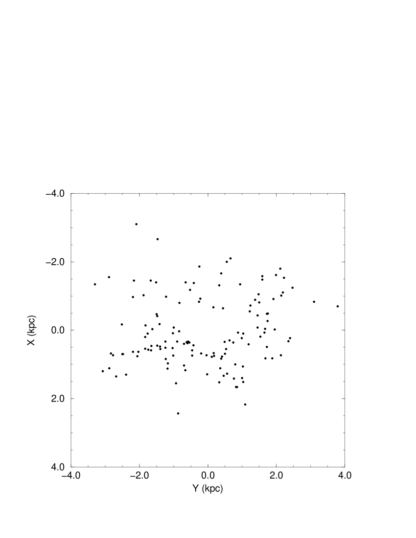
Our initial sample contains 6922 Hipparcos O- and B-type stars. The astrometric data for these stars come from the Hipparcos Catalogue (ESA ESA2 (1997)), radial velocities from the compilation of Grenier (Grenier (1997)) and Strömgren photometry from Hauck & Mermilliod’s (Hauck et al. (1998)) catalogue. The procedure followed to elaborate the sample considered here is fully described in Torra et al. (Torra et al. (2000); hereafter referred to as Paper I) along with a study of the possible biases in the trigonometric distances and the availability of radial velocities. Our sample contains 3915 stars with known distance and proper motions (2272 stars with known radial velocity). In Paper I we characterized the structure and kinematics of the Gould Belt system using this sample of O and B stars, establishing its boundary to a distance of about 0.6 kpc from the Sun. Taking into account the kinematic peculiarities of the Gould Belt, in this paper we do not consider those stars with kpc. In Fig. 1 we show the position of those stars with kpc projected on the galactic plane ( positive towards the galactic center and positive towards the galactic rotation direction), which is our working sample (448 stars; 307 of them with distance, radial velocity and proper motions and 141 with only distance and proper motions).

2.2 Sample of Cepheid stars
The initial sample contains all the Hipparcos classical Cepheids. Astrometric data were taken from the Hipparcos Catalogue (ESA ESA2 (1997)), whereas radial velocities come from Pont et al. (Pont et al.1 (1994), Pont et al.2 (1997)).
Individual distances were computed following two period-luminosity (PL) relations. In both, periods come from the Hipparcos Catalogue (ESA ESA2 (1997)) and individual reddenings from Fernie et al.’s (Fernie et al. (1995)) compilation (continuous updating). A classification between fundamental and overtone Cepheids from light curves and Fourier analysis was adopted (Beaulieu Beaulieu (1999)), using only the former in the kinematic analysis.
The first PL relation (Luri Luri (2000)) adopts a slope from EROS (Beaulieu Beaulieu (1999)) and corresponds to the short cosmic distance scale:
| (1) |
On the other hand, the second PL relation (Feast & Catchpole Feast et al.0 (1997)) corresponds to the large distance scale:
| (2) |
The sample contains 186 stars with known distance and proper motions (165 stars with radial velocity). Their distribution in the galactic plane (0.6 4 kpc) is shown in Fig. 2 (164 stars; 145 of them with distance, radial velocity and proper motions and 19 with only distance and proper motions).
3 A galactic kinematic model for the solar neighbourhood
3.1 Systematic velocity field in the galactic model
We propose an extension of the bidimensional model previously applied for radial velocities by Comerón & Torra (Comeron et al.1 (1991)). In our model we considered the systematic velocity components:
| (3) |
where subindex 1 refers to the solar motion contribution, subindex 2 to differential galactic rotation and subindex 3 to spiral arm kinematics, respectively (see Appendix A). Solar motion is expressed through the three components of the Sun’s velocity in galactic coordinates (). Galactic rotation curve was developed up to second-order approximation, and being the first- and second-order terms, respectively:
| (4) |
where we show the relationship between and the Oort constant. Oort constant can be derived from:
| (5) |
We considered as free parameters the galactocentric distance of the Sun () and the circular velocity at the Sun’s position (). Finally, spiral arm kinematics was modelled within the framework of Lin’s theory. We considered the number of the spiral arms () and their pitch angle () as free parameters, and we derived the perturbation velocity amplitudes in the antigalactocentric and tangential directions ( and , respectively; they were considered as constant magnitudes, assuming that their variation with the galactocentric distance is smooth), the phase of the spiral structure at the Sun’s position () and the parameter , which takes into account the difference in the velocity dispersion between the solar-type stars and the considered stars. This parameter is defined by the relationship between the spiral perturbation velocity amplitudes for the sample stars (, ) and for the Sun (, ):
| (6) |
where is the dimensionless rotation frequency of the spiral structure and is the stability Toomre’s number (Toomre Toomre (1969)), which depends on the velocity dispersion of the considered stars (see details in Appendix A). The inclusion of is new with regard to the model proposed by Comerón & Torra (Comeron et al.1 (1991)).
Eqs. (3.1) can be expressed as:
| (7) |
3.2 Free parameters of our galactic model
A 2-armed Galaxy was the first proposed view for our stellar system, mainly derived from HI and HII observations, but also from the spatial distribution of supergiant stars and other bright objects. These classical studies show the existence of at least two arms inside the solar circle (the Sagittarius-Carina or I arm and the Norma-Scutum or II arm), one local arm (Orion-Cygnus or 0 arm) and one external arm (Perseus or I arm). The Orion-Cygnus arm seems to be a local spur (Bok Bok (1958)). Lin et al. (Lin et al.2 (1969)) proposed a galactic system with 2 main spiral arms, where the Norma-Scutum and the Perseus arms are two segments of the same arm. By taking into account the interarm distance between the Sagittarius-Carina and the Perseus arms, these authors deduced a pitch angle of 6°. But, as early as the mid-70s, Georgelin & Georgelin (Georgelin et al. (1976)) proposed a 4-armed galactic system with a pitch angle of from a study of the spatial distribution of HII regions. However, Bash (Bash (1981)) examined this 4-armed model and found that a 2-arm pattern predicts HII regions in the same direction and with the same radial velocities as those used by Georgelin & Georgelin (Georgelin et al. (1976)), provided that dispersion velocities were considered.
In some recent papers several authors have also called this classical view in question. Vallée (Vallee (1995)) reviewed the subject of the determination of the pitch angle and the number of spiral arms and concluded that the Galaxy has a pitch angle of and that, taking into account the observed interarm distance, it would be a system of 4 spiral arms. This is also the opinion expressed by Amaral & Lépine (Amaral et al. (1997)), who, fitting the galactic rotation curve to a mass model of the Galaxy, found an autoconsistent solution with a system of 2 + 4 spiral arms (2 arms for 2.8 13 kpc and 4 arms for 6 11 kpc, with the Sun placed at 7.9 kpc) and a pitch angle of . Englmaier & Gerhard (Englmaier et al. (1999)) used the COBE NIR luminosity distribution and connected it with the kinematic observations of HI and molecular gas in - diagrams. They found a 4-armed spiral pattern between the corotation of the galactic bar and the solar circle. Drimmel (Drimmel (2000)) found that the galactic plane emission in the K band is consistent with a 2-armed structure, whereas the 240 m emission from dust is compatible with a 4-armed pattern. In a recent work, Lépine et al. (Lepine et al. (2001)) analyzed the kinematics of a sample of Cepheid stars and found the best fit for a model with a superposition of 2+4 spiral arms. Contrary to the model by Amaral & Lépine (Amaral et al. (1997)), Lépine et al. allowed the phase of both spiral patterns to be independent, deriving pitch angles of approximately and for and , respectively. They argued that this spiral pattern is in good agreement with the - diagrams obtained from observational HII data, though they admit that pure 2-armed model produces similar results. In the visible spiral structure of the Galaxy derived by Lépine et al. (see their Fig. 3) the Orion-Cygnus or local arm is seen as a major structure with a small pitch angle. In contrast, Olano (Olano (2001)) proposed that the local arm is an elongated structure of only 4 kpc of length and a pitch angle of about (in better agreement with the observational determinations of the inclination of the local arm found in the literature) formed from a supercloud about 100 Myr ago, when it entered into a major spiral arm.
In the case of the galactocentric distance of the Sun and the circular velocity at the Sun’s position there are also some inconsistencies among the different values found in the literature. In 1986, the IAU adopted the values 8.5 kpc and 220 km s-1 (Kerr & Lynden-Bell Kerr et al. (1986)). Recently, several authors have found values of nearly 7.5 kpc for (Racine & Harris Racine et al. (1989); Maciel Maciel (1993)). A complete review was done by Reid (Reid (1993)), who concluded that the most suitable value seems to be kpc. In kinematic studies there are serious discrepancies between different authors. Metzger et al. (Metzger et al. (1998)) found kpc and km s-1, whereas Feast et al. (Feast et al.2 (1998)) found kpc (both from radial velocities of Cepheid stars). Glushkova et al. (Glushkova et al. (1998)) found kpc from a combined sample including open clusters, red supergiants and Cepheids. Olling & Merrifield (Olling et al. (1998)) calculated mass models for the Galaxy and concluded that a consistent picture only emerges when considering kpc and km s-1. This value for the galactocentric distance of the Sun is in very good agreement with the only direct distance determination ( kpc), which was made employing proper motions of H2O masers (Reid Reid (1993)).
In the view of all that, we decided to derive the kinematic parameters of our model from different combinations of the free parameters involved. On the one hand, concerning spiral structure, two models of the Galaxy were considered: a first model with and , and a second one with and . Both models are consistent with an interarm distance of about 2.5-3 kpc, depending on the adopted value for the distance from the Sun to the galactic center. On the other hand, concerning the galactocentric distance of the Sun and the circular velocity at the Sun’s position, two different cases were also taken into account: a first one with kpc and km s-1, and a second one with kpc and km s-1. In both cases, the angular rotation velocity at the Sun’s position is km s-1 kpc-1.
4 Resolution of the condition equations
We determined the kinematic parameters of the galactic model via least squares fit from the equations:
| (8) |
where is the radial velocity of the star in km s-1, = 4.741 km yr (s pc )-1, is the heliocentric distance of the star in pc, and are the proper motion in galactic longitude and latitude of the star in ″ yr-1 and the galactic latitude. To derive the parameters , an iterative scheme extensively explained in Fernández (Fernandez (1998)) was followed.
The weight system was chosen as:
| (9) |
where are the individual observational errors in each velocity component of the star, calculated by taking into account the correlations between the different variables provided by the Hipparcos Catalogue, and is the projection of the cosmic velocity dispersion ellipsoid in the direction of the velocity component considered (see Paper I).
To check the quality of the least squares fits we considered the statistics for degrees of freeedom, defined as:
| (10) |
where are the independent data (sky coordinates and distances), the dependent data (radial and tangential velocity components), the number of equations and number of parameters to be fitted. According to Press et al. (Press et al. (1992)), if the uncertainties (cosmic dispersion and observational errors) are well-estimated, the value of for a moderately good fit would be , with an uncertainty of .
As we did in Paper I, to eliminate the possible outliers present in the sample due to both the existence of high residual velocity stars (Royer Royer (1997)) or stars with unknown large observational errors, we rejected those equations with a residual larger than 3 times the root mean square residual of the fit (computed as ) and recomputed a new set of parameters.
5 Test of robustness
The spiral arm potential is expected to contribute between 5-10% to the whole galactic gravitational field in the solar neighbourhood. This small contribution, and the large observational errors and constraints present on the spatial and kinematic parameters of distant stars, make it very difficult to quantify the kinematic perturbations induced by the spiral potential. Then, the results found in the literature have been characterised by significant uncertainties and discrepancies. A good example of this is the contradictory results obtained for the phase of the spiral structure at the Sun’s position (see Sect. 7.2): between arms or near an arm? Interesting questions to answer after the release of the Hipparcos data are:
-
•
How does the unprecedented astrometric precision provided by Hipparcos help to diminish such uncertainties? Are they small enough to measure the spiral arm kinematic parameters to any useful degree of accuracy?
-
•
Can we quantify the biases induced by our observational errors and constraints?
-
•
How can the correlations among variables present in the condition equations affect the kinematic parameters?
With regard to our stellar data, as seen in Sect. 2, both O and B star and Cepheid samples suffer from different observational limitations. Although the O and B star sample is large in number, it is limited in distance to no more than 1.5-2 kpc from the Sun (see Fig. 1 and Table 1). In contrast, the Cepheid sample reaches distances of up to about 4 kpc, but the number of stars with reliable data still remains very small (Fig. 2 and Table 1).
| sample of O and B stars | ||
|---|---|---|
| 0.1 2 kpc | 0.6 2 kpc | |
| 3418 (1903) | 448 (307) | |
| sample of Cepheid stars | ||
| 0.1 4 kpc | 0.6 2 kpc | 0.6 4 kpc |
| 119 (111) | 103 (95) | 164 (145) |
Numerical simulations were performed to answer the above questions, that is, to evaluate and quantify all the uncertainties and biases involved in our resolution process. In Appendix B we present the detailed procedure followed to build simulated samples as similar as possible to the real data for both O and B stars and Cepheids. This Appendix also contains an exhaustive analysis of the full set of cases which were simulated. Next we present the main conclusions arising from this work, which substantially contribute to the analysis of the real data:
-
•
As a general trend, owing to the correlations between variables, the biases and uncertainties in some kinematic parameters substantially vary when changing the real values of and .
-
•
The first- and second-order terms of the galactic rotation curve are accurately derived, with an uncertainty of less than 1.3 km s-1 kpc-1 (km s-1 kpc-2) in all cases. Whereas a negative bias for both parameters is detected for O and B stars (up to km s-1 kpc-1 for and km s-1 kpc-2 for ), it is negligible for Cepheids.
-
•
For the spiral structure parameters, we obtain better results from O and B stars than from Cepheids. This is due to the larger number of O and B stars. For both samples we found a clear dependence of some parameters with the assumed values for and . We can expect a bias in up to , and uncertainties of 10-20 for O and B stars and 30-60 for Cepheids. For and we found biases up to km s-1 and uncertainties of 1-2 km s-1. We did not find an important bias for neither for O and B stars nor Cepheids, though its standard deviation is large (4-10 km s-1 kpc-1 for O and B stars and 10-20 km s-1 kpc-1 for Cepheids). These ranges of values have allowed us to check how compatible are the results independently obtained for O and B stars and Cepheids.
-
•
If we choose an incorrect set of free parameters (, , , ), results change, but not to a large extent. This change is similar to the dispersion obtained when solving the condition equations from the different simulated samples (see Appendix B for details). Therefore, it will be difficult to decide between 2- and 4-armed models.
From these results, in Appendix B we conclude that, with the present available observational data, we are able to determine the kinematic parameters of the galactic model proposed in this paper, though we are not able to decide between a 2- or 4-armed Galaxy.
6 Results
In this section we present the results obtained from our working samples. To avoid those stars belonging to the Gould Belt, which can produce important deviations in our results (see Paper I), we always considered stars further than 0.6 kpc from the Sun. Following the results obtained in Appendix B, the working distance intervals are 0.6 2 kpc for O and B stars and 0.6 4 kpc for Cepheids.
A first set of results is presented in Table 2, considering a classical view of our galaxy (Lin et al. Lin et al.2 (1969); Kerr & Lynden-Bell Kerr et al. (1986)): we supposed a differential galactic rotation (, ) and a system with 2 spiral arms and a pitch angle of , the Sun placed at a galactocentric distance of 8.5 kpc a the circular velocity at the Sun’s position of 220 km s-1.
| O and B stars | Cepheid stars | ||
| 0.6 2 kpc | 0.6 4 kpc | ||
| SCS distances | LCS distances | ||
| 8.8 0.7 | 6.5 1.2 | 8.3 1.2 | |
| 12.4 1.0 | 10.4 1.9 | 9.3 2.1 | |
| 8.4 0.5 | 5.7 0.7 | 7.0 0.8 | |
| 1.3 1.0 | 8.1 1.2 | 4.5 1.1 | |
| 0.8 1.5 | 1.8 0.8 | 0.1 0.8 | |
| 45. 52. | 282. 20. | 306. 24. | |
| 1.6 1.1 | 0.1 1.6 | 0.7 1.4 | |
| 2.1 1.5 | 4.9 1.7 | 4.8 1.7 | |
| 0.42 0.10 | 0.96 0.01 | 0.96 0.01 | |
| 12.11 | 11.57 | 11.77 | |
| 2.07 | 0.84 | 0.84 | |
Although we do not only present solutions from radial velocity or proper motion data, we would like to remark that the parameters obtained when solving these cases (and comparing with the combined solutions presented in Table 2) are compatible between themselves within the errors bars. This is true for the sample of O and B stars and also in the case of the sample of Cepheids (for both short and large cosmic scales). Nevertheless, as we determined in Paper I, for this kind of kinematic analysis it is advisable to solve a combined resolution, in order to minimize the influence of the correlations present between the different parameters. This is especially important in the present case, since some correlations reach a large value (up to 0.8, though in the majority of cases they do not exceed 0.3). In Appendix B we check that these correlations do not impede our obtaining reliable results from our stellar samples.
If we compare the results obtained from O and B stars and Cepheids, we observe several discrepancies: differences up to 3.5 km s-1 kpc-1 in the Oort constant (derived from ) and up to 125 for the phase of the spiral structure at the Sun’s position. We must keep in mind that, whereas this parameter (like and ) is independent of the sample used, , and depend on the cosmic dispersion of the sample (thus, they do not have the same value for O and B stars and Cepheids).
As in Paper I, we found values of for O and B stars. We think that the difference from the expected value () could be due to an underestimation of the errors in the photometric distances and/or radial velocities for far stars. In the case of Cepheids we found values which agree with the expected .
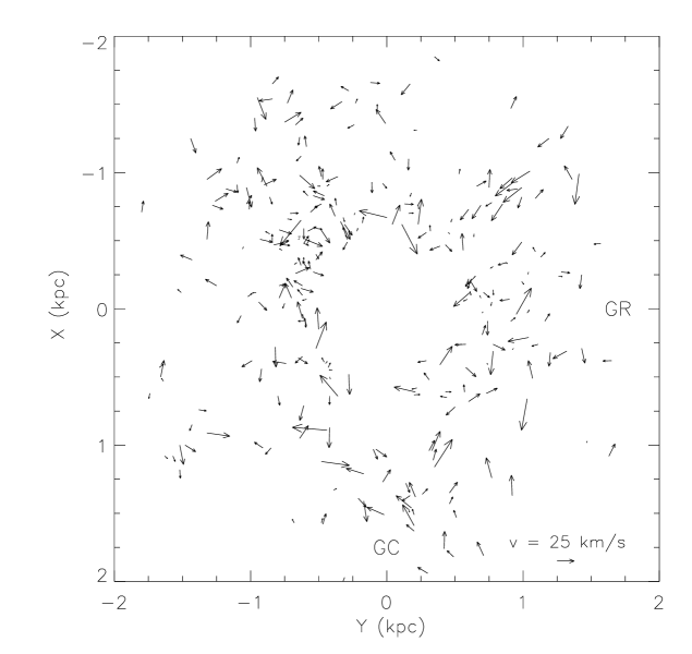
When studying the residuals of the equations we realized that radial velocity equations have a non-null average residual of about (3-4) km s-1 for both O and B stars and Cepheids. In the case of O and B stars (see Fig. 3) we can observe the peculiar motion of some OB associations. The kinematics of those associations located near the Sagittarius arm (e.g. Sgr OB1, Ser OB1 and Sct OB2, placed at ) were studied by Mel’nik et al. (Mel'nik et al.2 (1998)), who found that their motions are in general agreement with what would be expected according to Lin’s theory if these stars are located within the corotation radius. But we found these stars have a large residual, even taking into account in our model the galactic spiral structure, possibly due to the fact that they are still reflecting a motion peculiar to their birthplaces owing to their youth. Another region with a high residual is that located in the direction of the open clusters $h$ and $χ$ Per (NGC 869 and 884), at , where we observe a group of stars (distributed in an area of in the sky) with a high residual directed towards the Sun’s position. Thus, our results indicate that these stars do not fit the systematic velocity field defined by the whole sample. In this region of the sky the associations Per OB1 and Cas OB6 are to be found. The former is generally considered to include and Per and surrounding O and B stars. However, the stars in Fig. 3 have distances kpc, whereas the open clusters are located further on, at 2-2.5 kpc (Schild Schild (1967)). In our initial sample (see Sect. 2), we have in this region a group of stars with distances kpc, most of them belonging to Per OB1 according to the membership list done by Garmany & Stencel (Garmany et al. (1992)). But we did not use these stars in our kinematic analysis, due to their large distance errors. Garmany & Stencel (Garmany et al. (1992)) questioned if and Per really belong to Per OB1 due to the fact that B main sequence stars do not define a ZAMS at the distance of the open clusters. These authors derived a distance modulus of 11.8 ( kpc) for Per OB1 and 11.9 ( kpc) for Cas OB6. More recently, Mel’nik & Efremov (Mel'nik et al.1 (1995)) studied the spatial distribution of O and B stars within 3 kpc from the Sun and derived a new partition into OB associations using Battinelli’s (Battinelli (1991)) modification of the cluster analysis method. They found that Per OB1 split into four groups, two at kpc and another two at kpc. Two of them are reliable at a 90% confidence level (one at 1.6 kpc and another at 1.9 kpc), with a mean heliocentric radial velocity of km s-1 and km s-1, respectively. The first association found by Mel’nik & Efremov might correspond to the group of stars we have at kpc. In view of all that, the physical explanation of the large negative radial residuals present in this region, even considering the contribution from the spiral arm kinematics, is still unresolved.
If we exclude those stars belonging to both regions from our calculations, the average residual in radial velocity decreases to (1-2) km s-1. For Cepheids, as mentioned above, the residuals have the same trend and reach up to (3-4) km s-1, though in this case we cannot clearly identify groups of stars with a common motion. Therefore, the mean negative residual motion observed does not seem to be explained as the peculiar motion of some groups of stars. Moreover, we found that, for both samples, this residual motion apparently does not depend on the galatic longitude of the stars.
Taking into account that Cepheids, with a large mean distance, show larger residuals than O and B stars, we can suppose that this systematic trend could be explained through the addition of a -term in Eqs. (3.1), as developed in Paper I. Then, the following terms can be added to Eqs. (4):
| (11) |
which allow us to derive the parameter . Table 3 shows the results obtained in this way, and considering different sets of free parameters (as proposed in Sect. 3.2). The correlation coefficient between and the other parameters is always low, being smaller than 0.4 for O and B stars and 0.2 for Cepheids. As stated in Appendix B, a change in the value of the free parameters (, , and ) does not significantly alter the kinematic parameters derived. In Table 3 we also show the results when rejecting those stars belonging to the problematic regions mentioned above in the case of O and B stars. We observe that there is not a great difference in the results between these cases, which are always compatible within the errors. So, we conclude that the observed peculiar motion of some OB associations present in our sample does not alter the main parameters of our model. In view of that, in the next section we discuss the results obtained when considering all the stars, without rejecting associations.
| O and B stars with 0.6 2 kpc | ||||
| Case A | Case D | Case D | Case D | |
| excluding G1 | excluding G2 | |||
| 9.2 0.7 | 10.0 0.7 | 9.2 0.8 | 9.6 0.8 | |
| 12.7 1.1 | 12.7 1.0 | 13.2 1.0 | 12.3 1.1 | |
| 8.3 0.5 | 8.3 0.5 | 8.3 0.5 | 8.4 0.5 | |
| 1.7 1.0 | 1.5 1.0 | 2.3 1.2 | 0.9 1.0 | |
| 0.4 1.5 | 0.5 1.3 | 2.3 1.5 | 0.0 1.4 | |
| 3.2 0.7 | 2.8 0.7 | 1.4 0.7 | 2.4 0.7 | |
| 20. 53. | 329. 47. | 315. 32. | 8. 52. | |
| 3.1 1.1 | 2.6 1.0 | 3.2 1.1 | 2.8 1.1 | |
| 2.0 1.3 | 2.1 1.3 | 3.2 1.5 | 1.8 1.3 | |
| 0.23 0.57 | 0.35 0.25 | 0.40 0.10 | 0.19 0.77 | |
| 13.8 0.5 | 13.7 0.5 | 14.1 0.6 | 13.4 0.5 | |
| 12.7 0.8 | 13.2 0.7 | 14.1 0.8 | 13.0 0.7 | |
| 45. 14. | 33. 6. | 32. 3. | 36. 8. | |
| 3.6 1.6 | 1.5 0.9 | 1.1 0.6 | 2.0 1.2 | |
| 11.85 | 11.88 | 11.74 | 11.85 | |
| 1.89 | 1.90 | 1.90 | 1.89 | |
| Cepheid stars with 0.6 4 kpc | ||||
| SCS distances | LCS distances | |||
| Case A | Case D | Case A | Case D | |
| 6.5 1.2 | 6.5 1.2 | 8.4 1.2 | 8.2 1.2 | |
| 10.5 1.9 | 11.0 2.1 | 9.1 2.1 | 10.1 2.3 | |
| 5.7 0.7 | 5.7 0.8 | 7.0 0.8 | 7.0 0.8 | |
| 7.9 1.2 | 7.4 1.2 | 4.4 1.1 | 3.9 1.1 | |
| 1.6 0.8 | 0.5 0.8 | 0.1 0.8 | 0.9 0.8 | |
| 0.8 0.5 | 1.0 0.5 | 1.2 0.5 | 1.2 0.5 | |
| 286. 21. | 284. 39. | 310. 21. | 321. 43. | |
| 0.0 1.6 | 1.4 1.6 | 0.9 1.3 | 0.4 1.2 | |
| 4.8 1.7 | 2.4 1.7 | 5.6 1.7 | 2.7 1.7 | |
| 0.96 0.01 | 0.95 0.01 | 0.96 0.01 | 0.96 0.01 | |
| 16.9 0.6 | 16.6 0.6 | 15.1 0.6 | 14.9 0.6 | |
| 13.7 0.4 | 13.2 0.4 | 13.0 0.4 | 12.5 0.4 | |
| 26. 3. | 23. 4. | 28. 3. | 27. 2. | |
| 0.0 1.0 | 0.7 1.2 | 0.5 0.8 | 0.2 0.6 | |
| 11.56 | 11.66 | 11.70 | 11.90 | |
| 0.84 | 0.85 | 0.83 | 0.86 | |
7 Discussion
7.1 Galactic rotation curve
A difference in the Oort constant of approximately 3 km s-1 kpc-1 between solutions for O and B stars and Cepheids with short cosmic scale distances is obtained, whereas large cosmic scale provides an intermediate value:
| (12) |
As can be seen in Appendix B, these differences cannot be explained by the observational constraints present in both samples. A similar discrepancy was found by Frink et al. (Frink et al. (1996)), who derived km s-1 kpc-1 from a sample of O and B stars, and km s-1 kpc-1 from a sample of Cepheids (in both cases the authors only considered those stars with a heliocentric distance of less than 1 kpc). Nonetheless, our values for Cepheids do not reach the higher values obtained by Glushkova et al. (Glushkova et al. (1998); km s-1 kpc-1), Mishurov et al. (Mishurov et al.1 (1997); km s-1 kpc-1), Mishurov & Zenina (Mishurov et al.2 (1999); km s-1 kpc-1) and Lépine et al. (Lepine et al. (2001); km s-1 kpc-1). Pont et al. (Pont et al.1 (1994)) and Metzger et al. (Metzger et al. (1998)), from radial velocities of Cepheid stars, found values of km s-1 kpc-2 and km s-1 kpc-2, respectively. More recently, and using proper motions and distance calibration from Hipparcos data on Cepheid stars, Feast & Whitelock (Feast et al.1 (1997)) found a value of km s-1 kpc-1. Using a similar sample, Feast et al. (Feast et al.2 (1998)) found km s-1 kpc-1 from radial velocities. As we have mentioned in Sect. 6, we found good coherence for radial velocity, proper motion and combined solutions for both cosmic distance scales.
An attempt to explain these discrepancies was made by Olling & Merrifield (Olling et al. (1998)), who studied the variation of the and Oort functions and found that they significantly differ from the general dependence expected for a nearly flat rotation curve. Inside the solar circle, the value of rises to 18 km s-1 kpc-1 for kpc, disminishes to 16 km s-1 kpc-1 for kpc, and rises continuously for kpc, to 19 km s-1 kpc-1 for kpc (see Fig. 3 in Olling & Merrifield Olling et al. (1998)). Contrary to that, beyond the solar circle decreases to 10-12 km s-1 kpc-1, maintaining this value in the interval kpc. Although is a local parameter, describing the local shape of the rotation curve, Olling & Merrifield already pointed out that the discrepancies in the results published in the literature may be produced by their dependence on the galactocentric distance. Our O and B stars are distributed along all the galactic longitudes, whereas the Cepheids are predominantly concentrated inside the solar circle, with a peak in the spatial distribution for kpc corresponding to the Sagittarius-Carina arm (see Figs. 1 and 2). For O and B stars we found a classical value of km s-1 kpc-1 (a value between 10-12 and 16-18 km s-1 kpc-1), whereas for Cepheids a value 15-17 km s-1 kpc-1 (depending on the PL relation considered) was derived, in agreement with Olling & Merrifield’s assumptions.
From the results obtained in Appendix B, we would expect uncertainties in the second-order term of the rotation curve of km s-1 kpc-2 for O and B stars and km s-1 kpc-2 in the case of Cepheids. Taking this and the results in Table 3 into account, we can state that does not differ from a null value more than 2 km s-1 kpc-2. Pont et al. (Pont et al.1 (1994)) found a value km s-1 kpc-2, whereas Feast et al. (Feast et al.2 (1998)) found km s-1 kpc-2, both using radial velocities of Cepheid stars (the latter with a Hipparcos distance calibration). A large positive value was found by Lépine et al. (Lepine et al. (2001)), who derived km s-1 kpc-2 from their sample of Cepheid stars. As we will see in Sect. 7.2, these authors also found a large value for the amplitude of the velocity component in the galactic rotation direction due to the spiral potential (). Without specific simulations, considering both their observational data and resolution procedure, it is difficult to guess how the correlations between both parameters can affect their determination.
7.2 Spiral structure
Appendix B demonstrates that the available observational data allow the characterization of the galactic spiral structure, though the biases and uncertainties on the parameters have to be taken into account in the interpretation of the results. Furthermore, we realized that it is very difficult to establish the correct number of spiral arms of the Galaxy.
A first remarkable result is the fairly good coherence obtained for the phase of the spiral structure at the Sun’s position when using different free parameters (cases A, D) or different samples compared to the great discrepancies found in the literature (see below). We take into consideration that , and depend on the cosmic dispersion and so they do not have the same value for O and B stars and Cepheids.
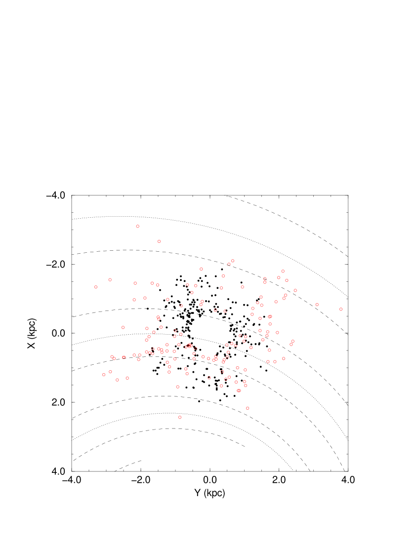
From Fig. 2, and assuming that Cepheids fairly trace the center of the Sagittarius-Carina arm, we can infer a value of 250 (the center of the inner visible spiral arm –the Sagittarius-Carina arm– at about 1 kpc from the Sun), depending on the exact value of the interarm distance. Nevertheless, the density wave theory predicts that the center of the visible arm (traced by its young stars) does not coincide with the position of the spiral potential minimum (Roberts Roberts1 (1969), Roberts2 (1970)). We must bear in mind that the kinematically derived value for informs us about the position of the Sun with respect this potential minimum, not with respect the visible arm. In Table 3 we found values inside the interval:
| (13) |
We take into consideration that in the minimum of the spiral potential (near the center of an arm) , whereas in the inner edge of the arm and in the outer edge . In the case of the phase of the spiral structure at the Sun’s position we expect a bias of for O and B stars and for Cepheids, with uncertainties of and , respectively (see Appendix B). These high uncertainties can explain the range of values obtained. According to the value found for , the Sun is located between the center and the outer edge of an arm, nearer to the former (see Fig. 4).
Our result stands in apparent contradiction to the classical mapping of the spiral structure tracers (Schmidt-Kaler Schmidt-Kaler (1975); Elmegreen Elmegreen (1985)), which locates the Sun in a middle position between the inner arm (Sagittarius-Carina arm) and the outer one (Perseus arm), that is, . The local arm (Orion-Cygnus arm) is normally considered as a local spur rather than a real arm. In our model, as we supposed an interarm distance of approximately 3 kpc, the local arm is also considered a local spur (see Sect. 3.2). But the value we obtained for differs significantly from . If we consider a difference of 30- between the optical tracers and the potential minimum of the spiral arm, we notice that our value is in good agreement with the picture of the spiral structure that emerges from the spatial distribution of stars in Fig. 4, with the inner spiral arm at approximately 1 kpc from the Sun. A similar result was obtained by Mel’nik et al. (Mel'nik et al.2 (1998)), who found that nearly 70% of the stars in the OB associations of the Sagittarius-Carina arm have a residual motion (after correcting their heliocentric velocities for solar motion and galactic rotation) in the direction opposite to the galactic rotation, as one would expect for those stars between the inner edge and the center of the arm. Then, they also found a shift between the optical position of the visible arm (traced by young stars) and the minimum of the spiral potential. Therefore, from our results we conclude that the Sun is placed relatively near the potential minimum of the Sagittarius-Carina arm, and the Perseus arm is located far away, at about 2.5 kpc from the Sun.
Our range of values for includes that obtained by Crézé & Mennessier (Creze et al. (1973)) from a sample of O-B3 stars, . Later, Mennessier & Crézé (Mennessier at al. (1975)) found from a sample of O-B3 stars a value of , which locates the Sun near the inner edge of an arm. Other authors obtained contradictory results. Gómez & Mennessier (Gomez et al. (1977)) found the Sun’s position near the edge of an arm from several samples of stars from FK4 and FK4 Supplement Catalogues. Byl & Ovenden (Byl et al. (1978)) and Comerón & Torra (Comeron et al.1 (1991)) obtained values of and respectively, from samples of O and B stars. Mishurov et al. (Mishurov et al.1 (1997)) found from a sample of Cepheid stars with radial velocities. Mishurov & Zenina (Mishurov et al.2 (1999)) found (supposing and kpc), from the same sample of Cepheid stars, but also including the Hipparcos proper motions. When these authors supposed they found . More recently, Rastorguev et al. (Rastorguev et al. (2001)) found from a sample of 55 open clusters younger than 40 Myr and 67 Cepheids with periods smaller than 9 days, all of them at kpc. We can see that there is poor agreement between the results published in the literature, though the last ones (the only ones with Hipparcos data) are all included in our range of possible values for .
The velocity amplitudes due to the spiral perturbation obtained are less than 4 km s-1 for O and B stars ( km s-1, 2-3 km s-1) and 6 km s-1 for Cepheid stars (-1 km s-1, 2-6 km s-1). The difference between results for O and B stars and Cepheids is explained by Lin’s theory as a result of their slight dependence on the galactocentric distance and the different cosmic dispersion for both samples. Mishurov et al. (Mishurov et al.1 (1997)) found km s-1 and km s-1 from their radial velocity data of Cepheid stars within 4 kpc from the Sun, supposing a 2-armed spiral pattern. Mel’nik et al. (Mel'nik et al.3 (1999)) found km s-1 and km s-1 from Cepheids within 3 kpc from the Sun. Mishurov & Zenina (Mishurov et al.2 (1999)) found km s-1 and km s-1 for and km s-1 and km s-1 for . From the same sample, Lépine et al. (Lepine et al. (2001)) found km s-1, km s-1 and km s-1, km s-1. Their 2+4-armed model yields large values for , implying a large value for the ratio between the spiral potential and the axisymmetric galactic field, much greater than that 5-10% normally accepted. According to the results obtained in Appendix B, the present observational uncertainties, biases and the correlations involved in the resolution procedure cannot completely explain the discrepancies among the values found in the literature. They can be attributed to our poor knowledge of the real wave harmonic structure of the galactic spiral pattern or to the approximation performed in the linear density-wave theory.
The derived angular rotation velocity of the spiral pattern is:
| (14) |
though there is a great dispersion around this value in our results from different samples and cases (dispersion of 2-7 km s-1 kpc-1, but up to 15 km s-1 kpc-1 in one extreme case). This is an expected dispersion, taking into account the results obtained in Appendix B (standard deviation of 2-5 km s-1 kpc-1 for O and B stars, but up to 15 km s-1 kpc-1 for ; for Cepheids dispersions are higher, of about 10-20 km s-1 kpc-1). Such a value places the Sun very near the corotation circle and is not in agreement with the classical km s-1 kpc-1 proposed by Lin et al. (Lin et al.2 (1969)). Nevertheless, other studies show results similar to ours. Avedisova (Avedisova (1989)) obtained km s-1 kpc-1 from the spatial distribution of young objects of different ages in the Sagittarius-Carina arm. More recently, Amaral & Lépine (Amaral et al. (1997)), working with a selection of young members of the open cluster catalogue by Mermilliod (Mermilliod (1986)), obtained a value of 20-22 km s-1 kpc-1. Mishurov et al. (Mishurov et al.1 (1997)) and Mishurov & Zenina (Mishurov et al.2 (1999)) used their sample of Cepheid stars and found km s-1 kpc-1 and km s-1 kpc-1, respectively. Lépine et al. (Lepine et al. (2001)) found km s-1 kpc-1 from their sample of Cepheid stars. Rastorguev et al. (Rastorguev et al. (2001)) thought that the evaluation of from kinematical data alone cannot be resolved. But our simulations (see Appendix B) seem to indicate that, at least, the tendency to find high values of is confirmed, though there is still an uncertainty of about 5-10 km s-1 kpc-1 in its value. These large values for can explain in a natural way the presence of a gap in the galactic gaseous disk (see Kerr Kerr (1969) and Burton Burton2 (1976) for observational evidences and Lépine et al. Lepine et al. (2001) for simulated results), since they placed the Sun near the corotation circle, where the gas is pumped out under the influence of the spiral potential.
7.3 The -term
In relation to the -term, we found good agreement between both O and B stars and Cepheids. A value of (1-3) km s-1 kpc-1 is found in all cases, confirming an apparent compression of the solar neighbourhood of up to 3-4 kpc. In our opinion, what most clearly proves the existence of a non-null value of is that it is independently found from the samples of O and B stars and Cepheids, which have a very different spatial distribution, an independent distance estimation and a different way of deriving their radial velocities. As we can see comparing Tables 2 and 3, the inclusion of the -term does not substantially modify the other model parameters derived by least squares fit.
It is very difficult to find in the literature other estimations of at these large heliocentric distances, since in the majority of cases authors consider an axisymmetric rotation curve. But some authors have pointed out the persistence of a residual in the radial velocity equations. Comerón & Torra (Comeron et al.2 (1994)) found km s-1 kpc-1 from O-B5.5 stars and km s-1 kpc-1 from B6-A0 stars with kpc. The radial velocity residual for Cepheids was first recognised by Stibbs (Stibbs (1956)). Pont et al. (Pont et al.1 (1994)) studied three possible origins for it: a statistical effect, an intrinsic effect in the measured radial velocities for Cepheids (-velocities) and a real dynamical effect. They finally suggested that it could be due to a non-axisymmetric motion produced by a central bar of kpc in extent. Metzger et al. (Metzger et al. (1998)) found a residual of km s-1 for a sample of Cepheids when considering an axisymmetric galactic rotation. They concluded that it might be due to the influence of spiral structure, not included in their model. However, in the present work we found a non-null value even taking into account spiral arm kinematics. An understanding of the physical explanation of the -term requires further study.
8 Conclusions
Hipparcos astrometric data were used to derive the spiral structure of the Galaxy in the solar neighbourhood. We considered two different samples of stars as tracers of this structure. In the sample of O and B stars the astrometric data were complemented with a careful compilation of radial velocities and Strömgren photometry, providing reliable distances and spatial velocities for these stars. In the sample of Cepheid stars we used two period-luminosity relations, one considering a short cosmic scale (Luri Luri (2000)) and another one standing for a large cosmic scale (Feast & Catchpole Feast et al.0 (1997)).
A kinematic model of our galaxy that takes into account solar motion, differential galactic rotation, spiral arm kinematics and a -term was adopted. The model parameters were derived via a classical weighted least squares fit. The robustness of our results was checked by means of careful insimulations.
A galactic rotation curve with a value of Oort constant of 13.7-13.8 km s-1 kpc-1 was found for the sample of O and B stars. In the case of Cepheid stars, we found 14.9-16.9 km s-1 kpc-1, depending on the case and the cosmic scale chosen. We confirmed the discrepancies appearing in when samples with a different distance horizon were used (Olling & Merrifield Olling et al. (1998)). For both cosmic scales we found an acceptable coherence between radial velocity, proper motion and combined solutions. Concerning the second-order term of the rotation curve, we always found a low value, compatible with zero.
The study of the residuals for radial velocity data made it evident that a -term was needed, which was found to be (1.4-3.2) km s-1 kpc-1 for O and B stars and (0.8-1.2) km s-1 kpc-1 for Cepheids. Although small, an apparent compression motion seems to exist in the galactic local neighbourhood for heliocentric distances up to 4 kpc, though its physical mechanism is still unknown.
The phase of the spiral structure at the Sun’s position obtained (-20) places it between the center and the outer edge of an arm. This is in good agreement with the spatial distribution of Cepheid stars. The angular rotation velocity of the spiral structure was found to be 30 km s-1 kpc-1, which places the Sun near the corotation circle.
Acknowledgements.
This work has been supported by the CICYT under contracts ESP 97-1803 and AYA 2000-0937. DF acknowledges the FRD grant from the Universitat de Barcelona (Spain).Appendix A systematic velocity components in the proposed galactic model
In this appendix we show the expressions of the velocity components in the three systematic contributions considered in our galactic model: solar motion, differential galactic rotation and spiral arm kinematics.
A.1 Solar motion
A star with galactic longitude and galactic latitude has the following radial and tangential velocity components owing to solar proper motion:
| (15) |
where , and are the components of the solar motion in galactic coordinates.
A.2 Galactic rotation
We consider axisymmetric differential rotation of our galaxy, with a rotation curve that can be developed in the solar neighbourhood as:
| (16) | |||||
where ( is the galactocentric distance of the Sun) and is the circular velocity at the Sun’s position. We note that allows us to calculate the Oort constant in the Sun’s vicinity:
| (17) |
The radial and tangential velocity components of a star in the galactic plane due to differential galactic rotation are:
| (18) | |||||
where is the galactocentric longitude of the star.
A.3 Spiral structure kinematics
Lin’s theory (Lin & Shu Lin et al.1 (1964); Lin et al. Lin et al.2 (1969); see also Rohlfs Rohlfs (1977)) assumes a spiral potential of the form:
| (19) |
( is the amplitude – – and is the phase of the density wave) which disturbs the axially symmetric gravitational potential. The shape of the spiral arms is well represented by a logarithmic spiral:
| (20) |
The amplitude is a slowly varying function of and the phase of the spiral structure can be related to the phase at the Sun’s position by the following expression:
| (21) |
where is the angular rotation velocity of the spiral pattern, the number of spiral arms and the pitch angle (for trailing spiral arms, 0). The phase of the spiral structure at the Sun’s position and the pitch angle can be determined from optical and radio indicators. Nevertheless, we point out that the maximum in the distribution of spiral arm tracers (position of the observed spiral arms) may be shifted in relation to the minimum in the perturbation potential (defined as ; see Roberts Roberts1 (1969)).
The mean peculiar velocities due to the spiral arm perturbations on the velocity field are, in the gas approximation, the following:
| (22) |
is positive towards the galactic anti-center and is positive towards the galactic rotation. In tightly wound spirals (i.e., those with ) the amplitudes and are slowly varying quantities with the galactocentric distance. is the radial wave number (for trailing spiral arms, 0):
| (23) |
is the dimensionless rotation frequency of the spiral structure, expressed in terms of the epicyclic frequency ():
| (24) |
(notice that in the region with , i.e. inner to the corotation circle). Furthermore:
| (25) |
and is the stability Toomre’s number (Toomre Toomre (1969)) defined as:
| (26) |
where is the velocity dispersion of the gas particles. Since the velocity amplitudes and depend on this velocity dispersion, we introduce a dimensionless parameter () that relates the velocity amplitudes of the Sun to those of the sample stars:
| (27) |
The so-called Lindblad resonances are defined as:
| (28) |
where the sign corresponds to the inner resonance and the sign to the outer one. In the region between both resonances (), is always positive and has a sign that depends on the sign of .
The amplitude of the spiral potential can be expressed as:
| (29) |
The maximum value of the radial force owing to this spiral potential is:
| (30) |
whereas the radial force due to the axisymmetric field is:
| (31) |
Therefore, the ratio between both quantities is:
| (32) |
The contributions in the radial and tangential velocity components of a star due to the spiral arm perturbation velocities and are the following:
A.4 Systematic velocity field in the proposed galactic model
The systematic radial and tangential velocity components of a star in our galactic model are given by:
| (34) |
where the constants contain combinations of the kinematic parameters that we wish to determine:
| (35) |
and are functions of the heliocentric distance and the galactic longitude and latitude:
| (36) |
In our resolution procedure the parameters are computed following an iterative scheme (extensively explained in Fernández Fernandez (1998)) and, from these, the kinematic parameters , , , , , , , and are derived.
With regard to the free parameters of our model, different values for , , , were considered (see Sect. 7).
Appendix B simulations to check the kinematic analysis
In Paper I we did numerical simulations in order to evaluate the biases in the kinematic model parameters (in that case, the Oort constants and the solar motion components) induced by our observational constraints and errors. In the present work, we have also generated simulated samples in the same way, though the significant correlations detected between some parameters make it advisable, in this case, to carry out a more detailed study.
In this section we present the process used to generate the simulated samples (the same as in Paper I, except for the change in the systematic contributions considered), the results we obtained and, finally, the quantification of the biases present in our real samples.
B.1 Process used to generate the simulated samples
To take into account the irregular spatial distribution of our stars and their observational errors, parameters describing the position of each simulated pseudo-star were generated as follow:
-
•
From each real star we generated a pseudo-star that has the same nominal position –not affected by errors– as the real one.
-
•
We assumed that the angular coordinates () have negligible observational errors.
-
•
The distance error of the pseudo-star has a distribution law:
(37) where is the individual error in the photometric distance of the real star ().
To generate the kinematic parameters we randomly assigned to each pseudo-star a velocity by assuming a cosmic dispersion and a Schwarzschild distribution:
| (38) |
where are the reflex of solar motion. These components were transformed into radial velocities and proper motions in galactic coordinates using the nominal position of the pseudo-star . The systematic motion due to galactic rotation and spiral arm kinematics was added following Eqs. (A.2) and (A.3), obtaining the components for each pseudo-star. Finally, individual observational errors were introduced by using the error function:
| (39) |
where , and are the observational errors of the real star.
At the end of this process we had the following data for each pseudo-star: galactic coordinates (), velocity parameters (), errors in the velocity parameters () and error in the photometric distance (). The simulated radial component of those pseudo-stars generated from a real star without radial velocity was not used, thus we imposed on the simulated sample the same deficiency in radial velocity data that is present in our real sample (see Sect. 2.2 and Appendix B in Paper I for more details).
Following this scheme, several sets of 50 simulated samples for both O and B stars and Cepheids were built. A classical solar motion of km s-1 was considered, taking the dispersion velocity components km s-1 for O and B stars (see Paper I) and km s-1 for Cepheids (Luri Luri (2000)). For the galactic rotation parameters, we chose the values km s-1 kpc-1 and km s-1 kpc-2, which correspond to a linear rotation curve with an Oort constant of 14.0 km s-1 kpc-1. On the other hand, for the spiral structure parameters several sets of values were used for (from to , in steps of ) and (from km s-1 kpc-1 to km s-1 kpc-1, in steps of 5 km s-1 kpc-1), whereas a fixed value of was considered (Yuan Yuan (1969)). From , , and , the values of , and were inferred for each set of samples.
56 sets of 50 samples for both O and B stars and Cepheids were generated. Concerning the free parameters of our model, in a first stage we adopted classical values (, , Lin et al. Lin et al.2 (1969); kpc, km s-1, Kerr & Lyndell-Bell Kerr et al. (1986)), though we also tested cases with , (Amaral & Lépine Amaral et al. (1997)) and kpc, km s-1 (Olling & Merrifield Olling et al. (1998)). In Table 4 we summarize all the adopted kinematic parameters.
| 9 km s-1 | |
| 12 km s-1 | |
| 7 km s-1 | |
| km s-1 (O and B stars) | |
| km s-1 (Cepheid stars) | |
| 2.1 km s-1 kpc-1 | |
| 0.0 km s-1 kpc-2 | |
| 0.05 | |
| from 0 to 360, | |
| in steps of 45 | |
| from 10 km s-1 kpc-1 to 40 km s-1 kpc-1, | |
| in steps of 5 km s-1 kpc-1 | |
| Case A | , , |
| kpc, km s-1 | |
| Case B | , , |
| kpc, km s-1 | |
| Case C | , , |
| kpc, km s-1 | |
| Case D | , , |
| kpc, km s-1 |
B.2 Results and discussion
B.2.1 Results for a 2-armed model of the Galaxy
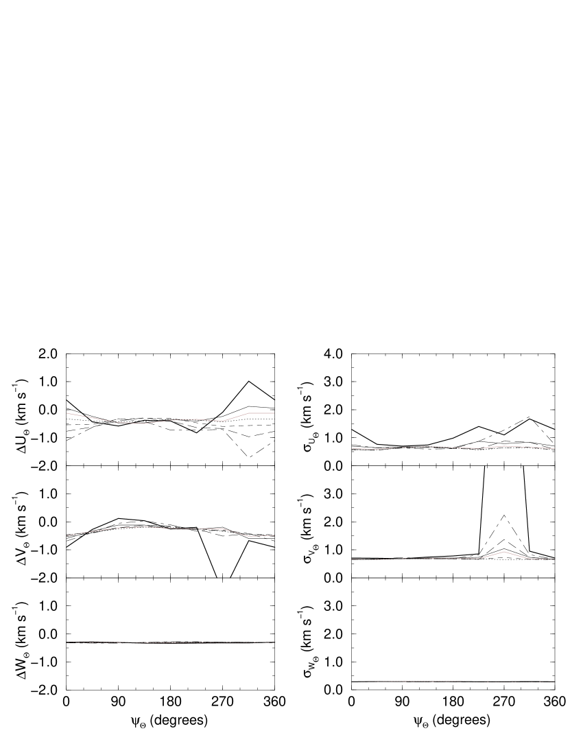
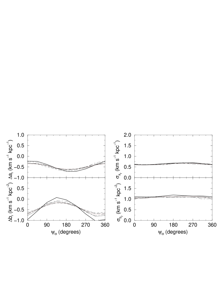
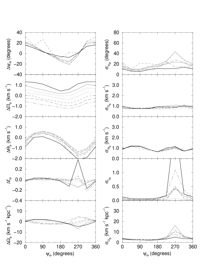
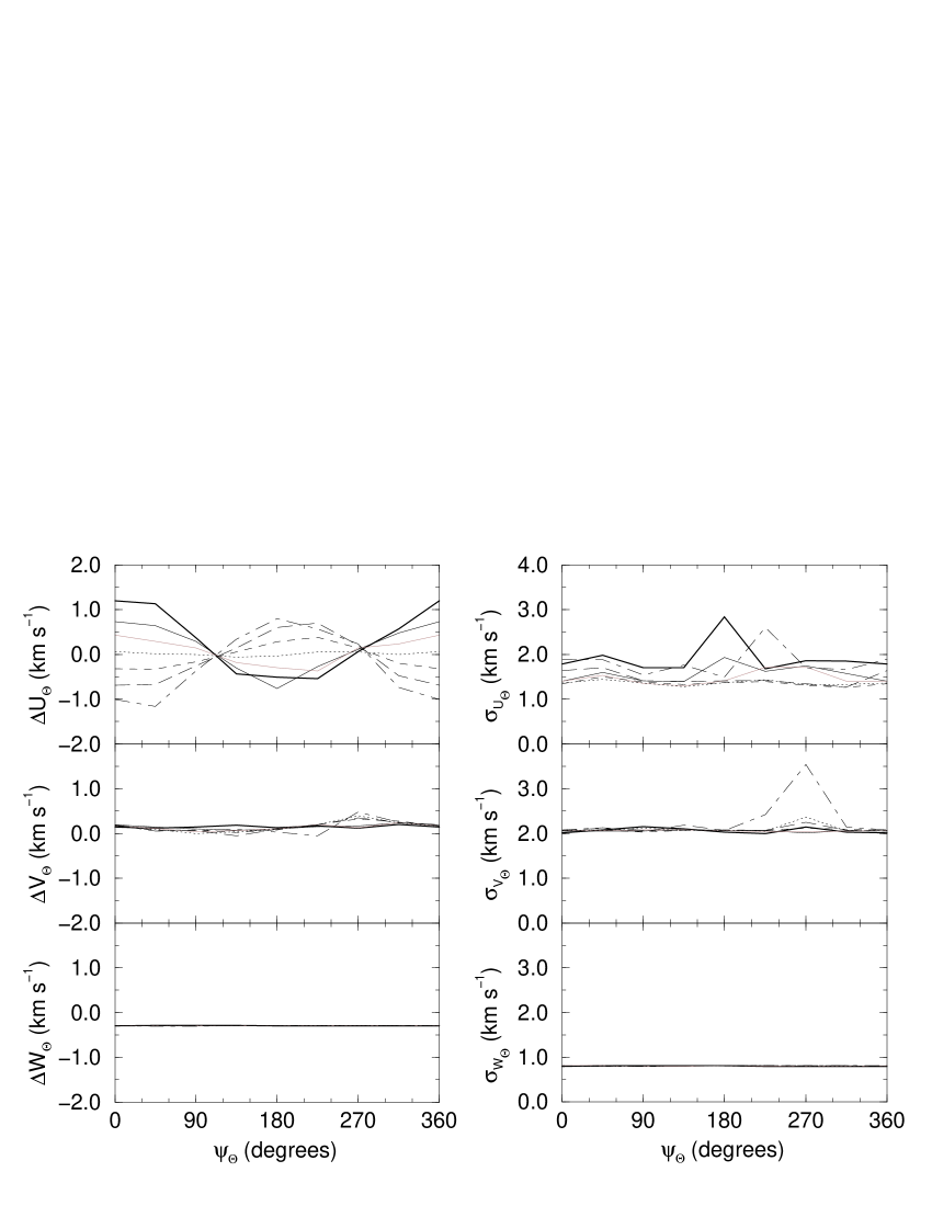
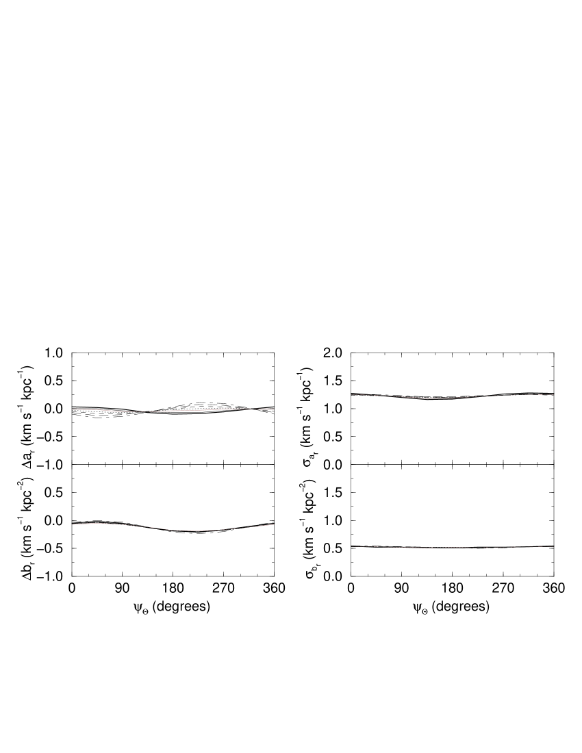
A complete solution simultaneously taking into account radial velocity and proper motion data was computed. Our test showed that the number of Cepheids within 2 kpc from the Sun prevents the obtainment of reliable results. In Figs. 5 and 6 we show the results obtained for the simulated samples of O and B stars (0.6 2 kpc) and Cepheids (0.6 4 kpc) in case A (see Table 4).
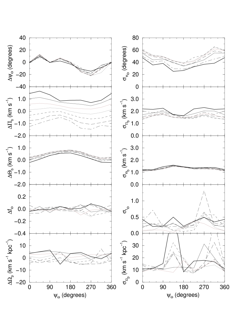
As a first conclusion, and confirming our suspicions, a systematic trend with and/or is observed in most cases. This behaviour is produced by the correlations between some terms in the least squares fit, which depends on the spatial distribution of each sample.
For solar motion a bias between and km s-1 (depending on and ) was found for and , and of only km s-1 for . For both O and B stars and Cepheids we found the bias on and to be independent of , with a slight dependence on . For and km s-1 kpc-1 we found a large negative bias on , but with a great standard deviation. This occurred in several samples (inside this set) with serious convergence problems in the iteration procedure we use to solve the least squares fit. Similar problems in other cases with will be found later. For O and B stars, the standard deviations in the solar motion components are km s-1 for and (except for ), and km s-1 for . On the other hand, in the case of Cepheids these values increased to 1.4-2.0 km s-1 and km s-1, respectively.
The biases found in the first- and second-order terms of the galactic rotation curve are negligible for Cepheids, with a level fluctuation of km s-1 kpc-1 (or km s-1 kpc-2). In this case there is a standard deviation of 1.3 for and 0.5 for . For O and B stars the biases clearly depend on , varying from to km s-1 kpc-1 for , and from to km s-1 kpc-2 for . The standard deviations are 0.8 km s-1 kpc-1 and 1.2 km s-1 kpc-2, respectively.
Let us study the biases that have an effect on the determination of the spiral structure parameters. As a general conclusion, Figs. 5 and 6 show that our sample of O and B stars supplies better results than the Cepheid sample.
In the case of O and B stars, we found a clear dependence with and in , and determinations, whereas and only show peculiar behaviour around . Concerning , the bias oscillates from to . The standard deviation of the mean for the 50 samples of each set is about 10-. On the other hand, for the amplitudes and the biases are of km s-1, with a standard deviation of about 1 km s-1. Neither nor have a considerable bias, except for , where both biases and standard deviations go up.
For Cepheid stars similar results were obtained, but with larger standard deviations in all cases. The bias in changes from to , with standard deviations of about 30-. In the case of , we found a clear dependence on both and , with a bias of km s-1 and a standard deviation of about 2 km s-1. On the other hand, for the bias is smaller, from 0 to 0.8 km s-1, and the standard deviation is 1-1.5 km s-1. As for O and B stars, for and small biases are found, though the standard deviations are larger in this case.
B.2.2 Results considering possible errors in the choice of the free parameters
An interesting point to analyse is the study of the biases produced by a bad choice of the free parameters in our model (, , , ). In the same way as in the previous section, we simulated 50 samples for each one of the cases considered in the real resolution, i.e. cases A, B, C and D (see Table 5). The simulated parameters were the same as in Table 4 for solar motion and galactic rotation. For spiral arm kinematics, we considered and km s-1 kpc-1 (similar values to those obtained from real samples; see Sect. 6).
| O and B stars with 0.6 2 kpc | Cepheid stars with 0.6 4 kpc | |||||||
| Case A | Case B | Case C | Case D | Case A | Case B | Case C | Case D | |
| Case A simulated | ||||||||
| 23. | 17. | 24. | 19. | 11. | 0. | 2. | 3. | |
| 28. | 27. | 25. | 25. | 65. | 61. | 71. | 71. | |
| 2.2 | 3.1 | 1.1 | 0.8 | 4.3 | 3.5 | 2.5 | 4.0 | |
| 6.2 | 7.3 | 2.9 | 3.5 | 18.9 | 16.6 | 8.8 | 7.3 | |
| Case B simulated | ||||||||
| 32. | 24. | 32. | 25. | 0. | 4. | 11. | 1. | |
| 34. | 32. | 31. | 30. | 83. | 75. | 82. | 78. | |
| 0.7 | 1.9 | 1.6 | 1.3 | 4.3 | 14.3 | 4.3 | 4.1 | |
| 7.1 | 8.0 | 3.8 | 3.9 | 16.2 | 52.8 | 7.0 | 8.1 | |
| Case C simulated | ||||||||
| 18. | 14. | 17. | 14. | 4. | 2. | 2. | 10. | |
| 24. | 23. | 21. | 21. | 62. | 58. | 60. | 63. | |
| 6.7 | 8.2 | 1.2 | 2.0 | 2.4 | 1.1 | 1.0 | 3.0 | |
| 6.5 | 7.3 | 2.9 | 3.3 | 25.1 | 21.5 | 10.9 | 9.2 | |
| Case D simulated | ||||||||
| 29. | 23. | 25. | 21. | 9. | 10. | 9. | 1. | |
| 31. | 29. | 27. | 26. | 84. | 78. | 81. | 73. | |
| 4.3 | 6.3 | 0.2 | 1.1 | 3.9 | 4.9 | 3.2 | 2.8 | |
| 7.1 | 8.2 | 3.7 | 3.8 | 17.1 | 19.5 | 7.8 | 8.6 | |
In Table 5 we show the biases and standard deviations when solving the model equations in crossed solutions (e.g. we generated 50 simulated samples considering the free parameters in case A, and then we solved equations using the free parameters adopted for cases A, B, C and D, and so on for the other cases). As a first conclusion, we can observe that a bad choice in the free parameters does not substantially alter the derived kinematic parameters, particularly . In other words, for each set of simulated samples we obtained nearly the same values for the parameters whether we solved the Eqs. (4) with the correct set of free parameters or with a wrong combination of them. Differences in do not exceed 10 for O and B stars and 20 for Cepheids. In the case of we found large differences in some cases, but always when the standard deviation was also large. This is especially true for Cepheids. A remarkable point is that the minimum bias was not always produced when we properly chose the free parameters.
B.2.3 Conclusions
In the light of these results, we conclude that we are able to determine the kinematic parameters of the proposed model of the Galaxy from the real star samples described in Sect. 2, supposing that the velocity field of the stars is well described by this model. We studied case A (, , kpc, km s-1 in detail in these simulations, but we also looked at the other combinations of the free parameters (cases B, C and D), with similar conclusions. Nevertheless, the study of crossed solutions has shown that it will be very difficult to decide between the several set of free parameters discussed in Sect. 6 (see also Table 5), owing to the small differences obtained when changing the free parameters in the condition equations.
References
- (1) Amaral, L.H., & Lépine, J.R.D. 1997, MNRAS, 286, 885
- (2) Avedisova, V.S. 1989, Astrophysics (Tr. Astrofizika), 30, 83
- (3) Bash, F.N. 1981, ApJ, 250, 551
- (4) Battinelli, P. 1991, A&A, 244, 69
- (5) Beaulieu, J.-P. 1999, private communication
- (6) Bok, B.J. 1958, Observatory, 79, 58
- (7) Bok, B.J., & Bok, P.F. 1974, The Milky Way, Cambridge, Harvard University Press
- (8) Burton, W.B. 1971, A&A, 10, 76
- (9) Burton, W.B. 1976, ARA&A, 14, 275
- (10) Byl, J., & Ovenden, M.W. 1978, ApJ, 225, 496
- (11) Comerón, F., & Torra, J. 1991, A&A, 241, 57
- (12) Comerón, F., Torra, J., & Gómez, A.E. 1994, A&A, 286, 789
- (13) Crézé, M., & Mennessier, M.O. 1973, A&A, 27, 281
- (14) Drimmel, R. 2000, A&A, 358, L13
- (15) Elmegreen, D.M. 1985, The Milky Way galaxy, eds. H. van Wörden, R.J. Allen, W.B. Burton, IAU Symposium 106, 255
- (16) Englmaier, P., & Gerhard, O. 1999, MNRAS, 304, 512
- (17) ESA 1997, The Hipparcos Catalogue, ESA SP-1200
- (18) Feast, M.W., & Catchpole, R.M. 1997, MNRAS, 286, L1
- (19) Feast, M.W., & Whitelock, P.A. 1997, MNRAS, 291, 683
- (20) Feast, M.W., Pont, F., & Whitelock, P.A. 1998, MNRAS, 298, L43
- (21) Fernández, D. 1998, Degree of Physics (Master Thesis), Universitat de Barcelona, Spain (available in Spanish language from http://www.am.ub.es/dfernand)
- (22) Fernie, J.D., Beattie, B., Evans, N.R., & Seager, S. 1995, IBVS, 4148
- (23) Frink, S., Fuchs, B., Röser, S., & Wielen, R. 1996, A&A, 314, 430
- (24) Garmany, C.D., & Stencel, R.E. 1992, A&AS, 94, 211
- (25) Georgelin, Y.M., & Georgelin, Y.P. 1976, A&A, 49, 57
- (26) Gómez, A., & Mennessier, M.O. 1977, A&A, 54, 113
- (27) Glushkova, E.V., Dambis, A.K., Mel’nik, A.M., & Rastorguev, A.S. 1998, A&A, 329, 514
- (28) Grenier, S. 1997, private communication
- (29) Hauck, B., & Mermilliod, J.C. 1998, A&AS, 129, 431
- (30) Kerr, F.J. 1969 ARA&A, 7, 39
- (31) Kerr, F.J., & Lynden-Bell, D. 1986, MNRAS, 221, 1023
- (32) Lépine, J.R.D., Mishurov, Yu.N., & Dedikov, S.Yu. 2001, AJ, 546, 234
- (33) Lin, C.C., & Shu, F.H. 1964, ApJ, 140, 646
- (34) Lin, C.C., Yuan, C., & Shu, F.H. 1969, ApJ, 155, 721
- (35) Luri, X., 2000, private communication
- (36) Maciel, W.J. 1993 Ap&SS, 206, 285
- (37) Marochnik, L.S., Mishurov, Yu.N., & Suchkov, A.A. 1972, Ap&SS, 19, 285
- (38) Mel’nik, A.M., & Efremov, Yu.N. 1995, Astro. Lett., 21, 10
- (39) Mel’nik, A.M., Sitnik, T.G., Dambis, A.K., Efremov, Yu.N., & Rastorguev, A.S. 1998, Astro. Lett., 24, 594
- (40) Mel’nik, A.M., Dambis, A.K., & Rastorguev, A.S. 1999, Astro. Lett., 25, 518
- (41) Mennessier, M.O., & Crézé, M. 1975, in ”La dynamique des galaxies spirales”, colloque n∘241, Centre National de la Recherche Scientifique, Paris
- (42) Mermilliod, J.C. 1986, A&AS, 63, 293
- (43) Metzger, M.R., Caldwell, J.A.R., & Schechter, P.L. 1998, AJ, 115, 635
- (44) Mishurov, Yu.N., Zenina, I.A., Dambis, A.K., Mel’nik, A.M., & Rastorguev, A.S. 1997, A&A, 323, 775
- (45) Mishurov, Yu.N., & Zenina, I.A. 1999, A&A, 341, 81
- (46) Olano, C.A. 2001, AJ, 121, 295
- (47) Olling, R.P., & Merrifield, M.R. 1998, MNRAS, 297, 943
- (48) Pont, F., Mayor, M., & Burki, G. 1994, A&A, 285, 415
- (49) Pont, F., Queloz, D., Bratschi, P., & Mayor, M. 1997, A&A, 318, 416
- (50) Press, W.H., Teukolsky, S.A., Vetterling, W.T., & Flannery, B.P. 1992, Numerical Recipes, Cambridge University Press, Cambridge
- (51) Racine, R., & Harris, W.E. 1989, AJ, 98, 1609
- (52) Rastorguev, A.S., Glushkova, E.V., Zabolotskikh, M.V., & Baumgardt, H. 2001, Astronomical and Astrophysical Transactions, in press
- (53) Reid, M.J. 1993, ARA&A, 31, 345
- (54) Roberts Jr., W.W. 1969, ApJ, 158, 123
- (55) Roberts Jr., W.W. 1970, The spiral structure of our galaxy, eds. W. Becker, G. Contopoulos, IAU Symposium 38, 415
- (56) Rohlfs, K. 1977, Lectures in density waves, Springer-Verlag, Berlin
- (57) Royer, F. 1999, PhD Thesis, Observatoire de Paris-Meudon, France
- (58) Schild R. 1967, ApJ, 148, 449
- (59) Schmidt, M. 1965, Galactic structure, eds. A. Blaauw and M. Schmidt, University Chicago Press, Chicago
- (60) Schmidt-Kaler, T. 1975, Vistas Astron., 19, 69
- (61) Stibbs, D.W.N. 1956, MNRAS, 116, 453
- (62) Toomre, A. 1969, ApJ, 158, 899
- (63) Torra, J., Fernández, D., & Figueras, F. 2000, A&A, 359, 82 (Paper I)
- (64) Vallée, J.P. 1995, ApJ, 454, 119
- (65) Yuan, C. 1969, ApJ, 158, 889