Time Scales in Long GRBs

Abstract

We analyze a sample of bright long bursts and find that the pulses duration have a lognormal distribution while the intervals between pulses have an excess of long intervals (relative to lognormal distribution). This excess can be explained by the existence of quiescent times, long periods with no signal above the background. The lognormal distribution of the intervals (excluding the quiescent times) is similar to the distribution of the pulses width. This result suggests that the quiescent times are made by a different mechanism than the rest of the intervals. It also suggests that the intervals (excluding the quiescent times) and the pulse width are connected to the same parameters of the source. We find that there is a correlation between a pulse width and the duration of the interval preceding it. There is a weaker, but still a significant, correlation between a pulse width and the interval following it. The significance of the correlation drops substantially when the intervals considered are not adjacent to the pulse.

1 Introduction

The light curve of a long duration Gamma-Ray Burst (GRB) (Kouveliotou 1993) is usually complex, it is composed from several dozens of short (about 1sec) distinguishable pulses. The variability of these bursts has been already used (Sari & Piran, 1997; Fenimore, Ramirez & Sumner 1997) to suggest that internal shocks , rather than external shocks produce most GRBs (simple models of the latter cannot produce efficiently variable bursts). The recent discovery of correlation relating properties of the temporal structure with the burst luminosity offer possibility of deriving independent estimates of the redshift of GRBs (Stern, Poutanen & Svensson 1997, 1999; Norris , Marani & Bonnell 2000; Fenimore & Ramirez-Ruiz 2000; Reichart et al 2000).

The temporal properties of long duration GRBs , and specifically the pulses and intervals properties, were investigated in previous works (e.g. McBreen et.al. 1994, Li & Fenimore 1996, Norris et. al. 1996, Quilligan et. al. 1999). We present here a further study of the temporal properties of GRB light curves. Using a new algorithm (Nakar & Piran, 2001b), which is based on Li & Fenimore (1996), we analyze the distribution of the time intervals between pulses and the pulses width in long bright bursts. We find that the pulses width, $\delta t$, distribution is consistent with a lognormal distribution. The distribution of intervals between pulses, $\Delta t$, becomes lognormal, with a comparable width to the $\delta t$ distribution, provided that we eliminate intervals that contain quiescent times. Namely, long periods with no evidence of photon counts above the background, between periods of strong $\gamma$-ray emission (Ramirez & Merloni 2001, Nakar & Piran 2001a). In nature such a deviation from a lognormal distribution occurs when a different mechanism govern the high end tail of the distribution. The similarity between the pulses width and the intervals distributions suggest that both distributions are influenced by the same (source) physical parameters. In this case, we expect also a correlation between the pulse width and its adjacent intervals. We search for this correlation using 12 bursts which contain enough pulses for such analysis to be applicable. In all these bursts there is a significant correlation between the pulse width and the duration of the interval preceding it. A significant correlation between the pulse width and the following interval was found in 60% of the bursts. In all the bursts the significance of the correlation between the pulse width and the preceding interval was higher or equal to this of the following interval.

2 The Algorithm and the Data

We have applied a modified Li & Fenimore (1996) peak finding algorithm (Nakar & Piran 2001b) to a sample of 68 long bursts ($T_{90}>2sec$, where $T_{90}$ is the time required to accumulate from 5 to 95 per cent of the total counts). This algorithm searches for individual peaks in BATSE 64ms concatenate data. In the analysis we consider the sum of all four energy channels, i.e. E $>$ 25Kev. This data type includes the photon counts, in a 64ms time bins, from a few seconds before the bursts trigger until a few hundred seconds after the trigger. The minimal $\Delta t$ and $\delta t$ are 0.128sec in this resolution. Each peak the algorithm find corresponds to one pulse. We determine the pulse width and the interval between two maxima, which we define as the interval between pulses (Norris et. al. 1996, Li & Fenimore 1996). The algorithm also searches for quiescent times. The definition of minimal duration of a quiescent time is somewhat arbitrary (whether a single time bin with a count level of the background is a quiescent time or not). We demand that the average of ten bins would be at the background level to be considered as a quiescent time. Hence the minimal quiescent time in our analysis is about 1sec.

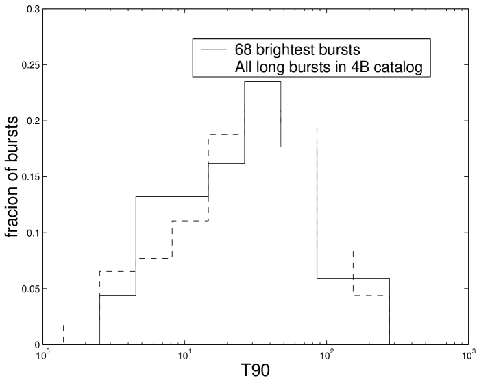
Figure 1: The normalized histogram of $T_{90}$ of the 68 brightest bursts (solid line), compared to the normalized histogram of all the long bursts in 4B catalog (dashed line).

The sample we consider is the 68 brightest long bursts in the BATSE 4B catalog (peak flux in 64ms$>$10.19$ph/(sec\cdot cm^{2})$). This resulted in 1330 pulses and 1262 intervals. The analysis below is based on the width of these pulses and the corresponding intervals between them.

One may wonder if the brightest bursts are representative. Figure 1 depicts the histogram of $T_{90}$ of our sample compared to the histogram of all the long bursts in 4B catalog. The histograms are similar. Therefore our sample, at least as far as duration is concerned, is representative for the entire 4B catalog.

We also analyze 24 dimmer bursts, which are still bright enough for the analysis to be carried out. These bursts are chosen randomly from the bursts with peak flux at 64ms greater than 4$ph/(sec\cdot cm^{2})$ but smaller than 10$ph/(sec\cdot cm^{2})$. This sample included 438 intervals. The results for this sample are consistent with those obtained for the brightest sample. Again indicating that the brightest sample is representative.

3 Temporal properties

3.1 Pulse Width Distribution

The distribution of the 1330 pulses’ widths is in excellent agreement with a lognormal distribution. The $\chi^{2}$ test gives a probability of $0.52$ that the data was taken from a lognormal distribution, with $\mu=0.065\pm 0.04$ ($\delta t_{avg}\approx 1sec$) and $\sigma=0.77\pm 0.03$ (corresponding at $1\sigma$ to 0.5- 2.3sec). Figure 2 depicts the histogram and the cumulative distribution of the pulses’ widths in the bright sample. The analysis of the dimmer sample (see sec 2) show also an excellent agreement with a lognormal distribution. The probability that the dimmer sample’s pulses width are taken from a lognormal distribution is 0.9.

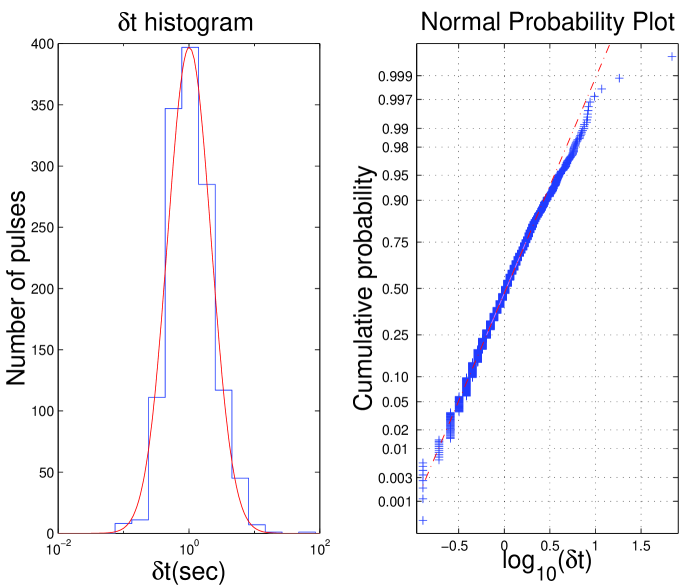
Figure 2: Left (a):The histogram of the pulses width, $\delta t$, compared with the best-fit Gaussian. Right (b): The cumulative distribution of $log_{10}(\delta t)$ compared with a normal distribution. Note that the excess of long pulses (top right) is due to a single pulse and it is not statistically significant.

3.2 Intervals Distribution and Quiescent Times

McBreen (1994) and Li & Fenimore (1996) suggested that the distribution of the intervals between pulses, $\Delta t$, is lognormal. We have found that the $\delta t$ distribution is lognormal. These results suggest that we consider first the null hypothesis that $\Delta t$ distribution is also lognormal.

Figure 3a depicts the histogram of the time intervals between neighboring peaks, $\Delta t$. Figure 3b shows the cumulative distribution of $log_{10}(\Delta t)$, compared to a best-fit Gaussian. Both figures show a clear excess of many long intervals. Using the $\chi^{2}$ test, we find a probability of $1.2\cdot 10^{-10}$ that the data was taken from a lognormal distribution. The null hypothesis clearly fails.

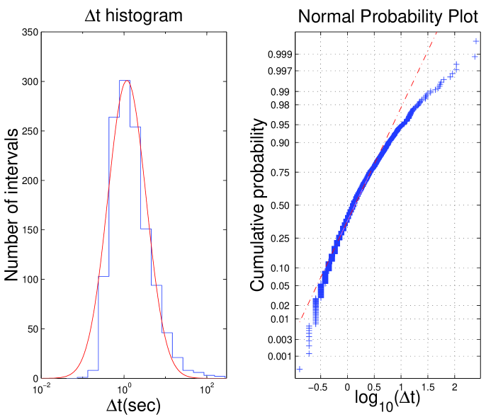
Figure 3: Left(a):The histogram of the time interval between neighboring peaks, $\Delta t$, compared with the best-fit Gaussian. Right(b): The cumulative distribution of $log_{10}(\Delta t)$ compared with a normal distribution.

Li & Fenimore (1996) already noticed such a deviation. A hints to this deviation could also be seen in the results presented by Norris et. al. (1996). Li & Fenimore (1996) and McBreen (personal communication 2000) have suggested that this deviation arises due to the limited resolution of the observations, and therefore the intervals distribution is consistent with a lognormal one. To test this hypothesis we examine in Figure 4 the cumulative probability of a mirror image of the right half of the $\Delta t$ histogram. This half is insensitive to the limited resolution. Again the figure show a deviation from a lognormal distribution and an excess of long intervals (and short ones which are of course the mirror of the long intervals). This indicates that $\Delta t$ distribution is not a lognormal.

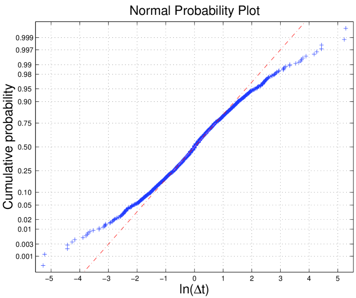
Figure 4: The cumulative distribution of all the intervals, $\Delta t$, above the median, compared with the best-fit Gaussian. The intervals above the median form only the right part of the distribution. The left half is a duplication of the right one. The entire sample is shifted by $ln(median(\Delta t))$ so it is symmetric around zero.

The analysis of the dimmer bursts sample (see sec. 2) gives similar results. Figure 5 shows the cumulative distribution of $log_{10}(\Delta t)$ in the dimmer sample compared to the best-fit Gaussian. The excess of long intervals is clear. The $\chi^{2}$ test gives a probability of $9\cdot 10^{-6}$ that this data was taken from a lognormal distribution.

Figure 5: The cumulative distribution of $log_{10}(\Delta t)$. $\Delta t$ is taken from the sample of 24 dimer bursts. The cumulative distribution is compared to this of a normal distribution with the best-fit parameters.

We found that the long intervals between neighboring peaks are often dominated by quiescent times. Such periods are seen in 35 of the bursts in our sample (all together there are 50 quiescent times). Most of the bursts contain one or two quiescent times, some contain three. The quiescent times last typically several tens of seconds and they range between a second (our arbitrary lower limit) to hundreds of seconds. In some bursts the quiescent times are a significant fraction of the total duration.

Since the quiescent times contribute to the duration of the longest intervals we examined the possibility that they cause the excess of long intervals (over a lognormal distribution). We examine the interval distribution excluding now all intervals that contained a quiescent time. Figure 6 shows the histogram and the cumulative distribution of $log_{10}(\Delta t)$ excluding the intervals that contained a quiescent time, compared to the best-fit Gaussian with $\mu=0.257\pm 0.051$ ($\Delta t_{avg}\approx 1.3sec$) and $\sigma=0.90\pm 0.04$ (corresponding at $1\sigma$ to 0.53-3.1sec). The fit is good. The $\chi^{2}$ test gives a probability of $0.27$ that this data was taken from a lognormal distribution. Moreover, the modified $\Delta t$ distribution has a comparable width to the $\delta t$ distribution (which is unaffected by quiescent times).

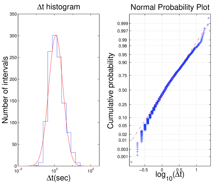
Figure 6: The histogram and cumulative distribution of time intervals between neighboring peaks, $\Delta t$, excluding intervals that contain quiescent times, compared with the best-fit Gaussian.

3.3 The Correlation Between Pulses and Neighboring Intervals

The similarity between the two distributions motivated us to explore the correlation between pulses and their neighboring intervals. We calculated Pearson’s linear correlation coefficient, $r$, and Spearman’s ranked order coefficient, $r_{s}$, between a pulse duration and the intervals just preceding it, and just following it (excluding intervals that contain a quiescent time). In order to avoid any influence of the algorithm on the correlation we considered here only well separated pulses, namely, pulses whose half maximum (used to determine the width) is above the minimum between the pulse and its neighbors. In this case there is no worry about overlap between the pulses that may introduce a spurious correlation.

We considered only bursts with more than 12 separated pulses, all together 12 bursts of our sample with an average of 23 pulses per burst. Our null hypothesis is of no correlation between the pulses width and the intervals. The probabilities of rejection of the null hypothesis found to be similar for both methods, $r$ and $r_{s}$. All the considered bursts showed a positive correlation between a pulse width and the preceding interval. The rejection of the null hypothesis is above 90% in half of the bursts and above 70% in the rest. The correlation between a pulse width and the following interval is less significant. In 5 of the bursts the null hypothesis is rejected with a confidence of more then 90%, and In 7 of the bursts the rejection confidence level is above 70%. In 4 bursts there is no evidence for correlation. In all the considered bursts the significance of the correlation between the pulse width and the preceding interval is higher or equal to the correlation with the following interval.

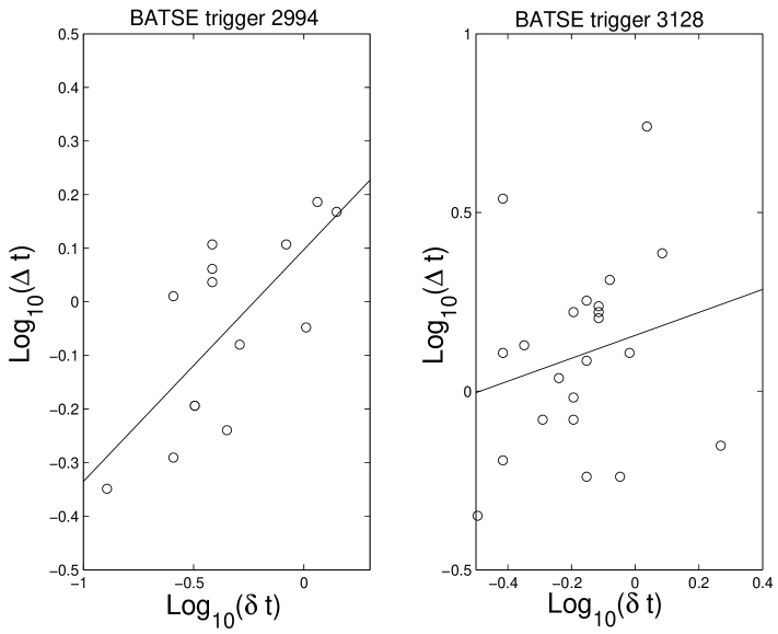
Figure 7: The pulses width and the preceding interval duration in BATSE triggers 2994 and 3128. Trigger 2994 has the most significant correlation between the two parameters in the analyzed bursts. The confidence level of this correlation is 99.5%. Trigger 3128 has the least significant correlation between the two parameters in the analyzed bursts. The confidence level of this correlation is 70%.

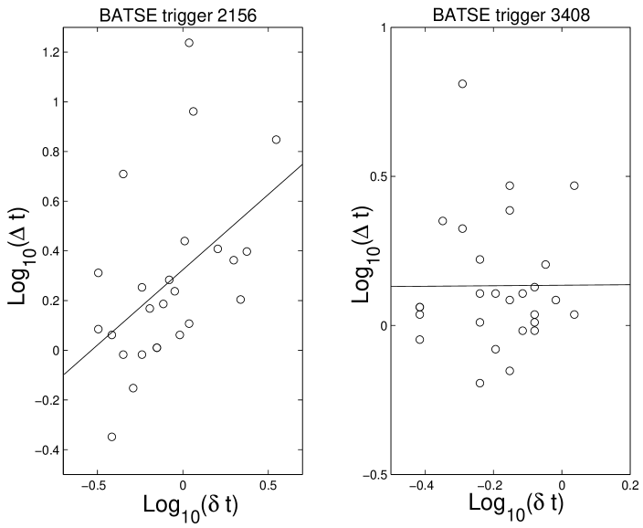
Figure 8: The pulses width and the following interval duration in BATSE triggers 2156 and 3408. Trigger 2156 has the most significant correlation between the two parameters in the analyzed sample. The confidence level of this correlation is 98.3%. There is no evidence for correlation between the two parameters in trigger 3408.

Figure 7 shows the pulses width and the preceding interval duration of the most correlated burst and the least correlated one. In both bursts a correlation is clearly seen. The best linear fit parameters of each burst are different, but the variance of the slope parameter is not large, compared with the typical slope. The average linear fit is $log(\Delta t)=(0.49\pm 0.19)\cdot log(\delta t)+(0.25\pm 0.11)$. Figure 8 shows the pulses width and the following interval duration of the most correlated burst and the least correlated burst. While the correlation is clearly seen in trigger 2156, there is no evidence for correlation in trigger 3408. The average Linear fit for the correlated bursts (significance level above 70%) is $log(\Delta t)=(0.55\pm 0.11)\cdot log(\delta t)+(0.26\pm 0.11)$.

The correlation disappears if we consider non neighboring intervals and pulses. For example, only half of the considered bursts show a positive correlation between a pulse duration and the interval after the following pulse. In no burst the rejection of the null hypothesis of no correlation is above 90%.

4 Discussion

The pulse duration distribution is consistent with a lognormal one. However, the distribution of the intervals between pulses is inconsistent with a lognormal distribution. Removal of the intervals that include quiescent times results in a distribution consistent with lognormal. This suggests that the distribution of interval between pulses is made of the sum of two different contributions. A lognormal distribution that is similar to the pulse width distribution, and the quiescent times distribution. The last one is dominant at the high end tail of the intervals distribution and produce the deviation from a lognormal distribution. We stress (see also Ramirez & Merloni 2001) that the quiescent times that we find here are not the same as the gaps between the precursors and the main pulses (Koshut et al, 1995) found in 3% of the bursts. In that case the gaps are between a softer and weaker component (the precursor) and a harder and much stronger one (the main burst). Here we observe gaps between pulses with the same characteristics. Moreover, in many cases we observe several quiescent times within the same burst.

The existence of quiescent times, and of two different mechanisms that control the gaps between pulses pose a new challenge to any model attempting to explain the temporal structure of GRBs. This suggests that there are three time scales of different nature within GRBs : (i) The shortest time scale, the variability scale which determines the pulses duration and the interval between pulses (both have a similar time-scale). (ii) An intermediate time scale producing long periods within the bursts with no activity (quiescent times). (iii) The longest time scale which corresponds to the duration of the burst.

Within the popular internal shock model the observed temporal structure reflects the activity of the “inner engine” (e.g. Kobayashi, Piran & Sari 1997; Ramirez & Fenimore, 2000). Within this model quiescent times reflect, most likely, periods in which the “inner engine” is not active at all. Alternatively they could reflect periods in which the “inner engine” emits a sequence of shells that do not collide (e.g. shells with a decreasing Lorentz factors) (Ramirez, Merloni & Rees 2000). In both cases the quiescent times correspond to periods in which the activity of the “inner engine” differs from its usual activity. Within the internal shocks model the shortest time scale corresponds to the variability of the “inner engine”, the quiescent periods time scale corresponds to periods of different activity of the “inner engine” and the duration of the burst corresponds to the total duration of activity of the “inner engine”.

We also find that the pulse duration is correlated to the preceding interval duration in all the analyzed bursts. A weaker but still significant correlation is found between the pulse duration and the following interval duration. This correlation was found only in 60% of the analyzed bursts.

While, different mechanisms can produce the observed lognormal distributions, the similarity between the pulse and interval distributions and the correlation between the pulses and neighboring intervals require that both processes would be determined by the same mechanism (or at least by two mechanisms governed by the same (source) physical parameters). This provides a new constraint on GRB models that should be considered in any model that attempts to reconstruct GRBs light curves.

For example, our results should be taken into account when choosing parameters in simulations of internal shocks light curves. Specifically, the parameters that determine the temporal characteristics of the relativistic wind should be chosen such that the resulting pulses and intervals would have lognormal distributions, with the appropriate parameters as well as quiescent times. In another paper (in preparation) we discuss the correlation between pulses and neighboring intervals within the internal shock model.

References

- [1] Fenimore E. E., Ramirez-Ruiz E., 2000 submitted to ApJ (astro-ph/0004176)
- [2] Fenimore E. E., Ramirez E.,Sumner M. C., 1997 in: Gamma-Ray Bursts, 4th Huntsville Symposium , Meegan, C., Preece, R., & Koshut, T., Eds., AIP Conf. Proc. NY p. 657
- [3] Kobayashi S., Piran T., Sari R., 1997, Apj, 490, 92
- [4] Koshut T. et al., ApJ, 1995, 452, 145
- [5] Kouveliotou C., Meegan C. A., Fishman G. J., Bhat N. P., Briggs M. S., Koshut T. M., Paciesas W. S., Pendleton G. N., 1993, ApJ, 413, L101
- [6] Li H., Fenimore E., 1996, ApJ, 469, L115
- [7] McBreen B., Hurley K. J., Long R., Metcalfe L., 1994, MNRAS, 271, 662
- [8] Nakar E., Piran T., 2001a, to appear in A&As, proceedings of the second Rome GRB meeting, astro-ph/0103011
- [9] Nakar E., Piran T., 2001b submitted to MNRAS, astro-ph/0103192
- [10] Norris J. P., Nemiroff R. J., Bonnell J. T., Scargle J. D., Kouveliotou C., Paciesas W. S., Meegan C. A., Fishman G. J., 1996, ApJ, 459, 393
- [11] Norris J. P., Marani G. F., Bonnell J. T., 2000, ApJ, 534, 248
- [12] Quilligan F., Hurley K. J., McBreen B., Hanlon L., Duggan P., 1999, A&AS, 138, 419
- [13] Ramirez-Ruiz E., Fenimore E. E., 2000, ApJ, 539, 712
- [14] Ramirez-Ruiz E., Merloni A., 2001, MNRAS, 320, L25
- [15] Ramirez-Ruiz E., Merloni A., Rees M. J., 2001, MNRAS, 324, 1147
- [16] Reichart D. E., Lamb D. Q., Fenimore E. E., Ramirez-Ruiz E., Cline T. L., Hurley K., 2001, ApJ, 552, 57
- [17] Sari R., Piran T., 1997, ApJ, 485, 270
- [18] Stern B., Poutanen J., Svensson R., 1997, ApJ, 489, L41
- [19] Stern B., Poutanen J., Svensson R., 1999, ApJ, 510, 312