X-ray, Optical, and Radio Observations of the Type II Supernovae 1999em and 1998S

Abstract

Observations of the Type II-P (plateau) Supernova (SN) 1999em and Type IIn (narrow emission line) SN 1998S have enabled estimation of the profile of the SN ejecta, the structure of the circumstellar medium (CSM) established by the pre-SN stellar wind, and the nature of the shock interaction. SN 1999em is the first Type II-P detected at both X-ray and radio wavelengths. It is the least radio luminous and one of the least X-ray luminous SNe ever detected (except for the unusual and very close SN 1987A). The Chandra X-ray data indicate non-radiative interaction of SN ejecta with a power-law density profile ($\rho\propto r^{-n}$ with $n\sim 7$) for a pre-SN wind with a low mass-loss rate of $\sim 2\times 10^{-6}$ M_⊙ yr^-1 for a wind velocity of 10 km s^-1, in agreement with radio mass-loss rate estimates. The Chandra data show an unexpected, temporary rise in the 0.4–2.0 keV X-ray flux at $\sim$100 days after explosion. SN 1998S, at an age of $>$3 years, is still bright in X-rays and is increasing in flux density at cm radio wavelengths. Spectral fits to the Chandra data show that many heavy elements (Ne, Al, Si, S, Ar, and Fe) are overabundant with respect to solar values. We compare the observed elemental abundances and abundance ratios to theoretical calculations and find that our data are consistent with a progenitor mass of approximately 15–20 M_⊙ if the heavy element ejecta are radially mixed out to a high velocity. If the X-ray emission is from the reverse shock wave region, the supernova density profile must be moderately flat at a velocity $\sim 10^{4}$ km s^-1, the shock front is non-radiative at the time of the observations, and the mass-loss rate is 1–2$\times 10^{-4}$ M_⊙ yr^-1 for a pre-supernova wind velocity of $10$ km s^-1. This result is also supported by modeling of the radio emission which implies that SN 1998S is surrounded by a clumpy or filamentary CSM established by a high mass-loss rate, $\sim 2\times 10^{-4}$ M_⊙ yr^-1, from the pre-supernova star.

Accepted by the Astrophysical Journal

1 Introduction

To date, 14 supernovae (SNe) have been detected in X-rays in the near aftermath (days to years) of their explosions: SNe 1978K (Petre et al., 1994; Schlegel, 1995; Schlegel, Petre, & Colbert, 1996; Schlegel, 1999a), 1979C (Immler, Pietsch, & Aschenbach, 1998a; Kaaret, 2001; Ray, Petre, & Schlegel, 2001), 1980K (Canizares, Kriss, & Feigelson, 1982; Schlegel, 1994, 1995), 1986J (Houck et al., 1998; Schlegel, 1995; Chugai, 1993; Bregman & Pildis, 1992), 1987A (Burrows et al., 2000; Dennerl et al., 2001; Gorenstein, Hughes, & Tucker, 1994; Hasinger, Aschenbach, & Trüumper, 1996), 1988Z (Fabian & Terlevich, 1996), 1993J (Immler, Aschenbach, & Wang, 2001; Suzuki & Nomoto, 1995; Zimmermann et al., 1994), 1994I (Immler, Pietsch, & Aschenbach, 1998b; Immler, Wilson, & Terashima, 2002), 1994W (Schlegel, 1999b), 1995N (Fox et al., 2000), 1998bw (aka GRB 980425; Pian et al. 1999; Pian et al. 2000), 1999em (Fox et al., 1999; Schlegel, 2001a), and 1999gi (Schlegel, 2001b). We present here results from Chandra observations of SN 1999em and SN 1998S. In general, the high X-ray luminosities of these 14 SNe ($\mbox{$L_{\rm x}$}\sim 10^{38}$–10⁴¹ ergs s^-1) dominate the total radiative output of the SNe starting at an age of about one year. This soft X-ray ($\lesssim 10$ keV) emission is most convincingly explained as thermal radiation from the “reverse shock” region that forms within the expanding SN ejecta as it interacts with the dense stellar wind of the progenitor star.

The interaction of a spherically symmetric SN shock and a smooth circumstellar medium (CSM) has been calculated in detail (Chevalier & Fransson, 1994; Suzuki & Nomoto, 1995). As the SN “outgoing” shock emerges from the star, its characteristic velocity is $\sim$10⁴ km s^-1, and the density distribution in the outer parts of the ejecta can be approximated by a power-law in radius, $\rho\propto r^{-n}$, with $7\lesssim n\lesssim 20$. The outgoing shock propagates into a dense CSM formed by the pre-SN stellar wind. This wind is slow ($v_{w}\sim 10~{}\mbox{km s${}^{-1}$}$) and was formed by a pre-supernova mass-loss rate of $\dot{M}\sim 10^{-4}$ to $10^{-6}$ M_⊙ yr^-1. The CSM density for such a wind decreases as the square of the radius ($\rho=\dot{M}/4\pi r^{2}v_{w}$). The collision between the stellar ejecta and the CSM produces a “reverse” shock, which travels outward at $\sim$10³ km s^-1 slower than the fastest ejecta. Interaction between the outgoing shock and the CSM produces a very hot shell ($\sim$10⁹ K) while the reverse shock/ejecta interaction produces a denser, cooler shell ($\sim$10⁷ K) with much higher emission measure and is where most of the observable X-ray emission arises. If either the CSM density or $n$ is high, the reverse shock is radiative, resulting in a dense, partly-absorbing shell between the two shocks.

Chevalier (1982) proposed that the outgoing shock from the SN explosion generates the relativistic electrons and enhanced magnetic field necessary for synchrotron radio emission. The ionized CSM initially absorbs most of this emission, except in cases where synchrotron self-absorption dominates, as may have been the case in SN 1993J (Chevalier, 1998; Fransson & Björnsson, 1998). However, as the shock passes rapidly outward through the CSM, progressively less ionized material is left between the shock and the observer, and absorption decreases rapidly. The observed radio flux density rises accordingly. At the same time, emission from the shock region is decreasing slowly as the shock expands so that, when radio absorption has become negligible, the radio light curve follows this decline. Observational evidence also exists at optical wavelengths for this interaction of SN shocks with the winds from pre-supernova mass loss (Filippenko, 1997).

All known radio supernovae appear to share common properties of (i) non-thermal synchrotron emission with a high brightness temperature, (ii) a decrease in absorption with time, resulting in a smooth, rapid turn-on first at shorter wavelengths and later at longer wavelengths, (iii) a power-law decline of the emission flux density with time at each wavelength after maximum flux density (absorption $\tau\approx 1$) is reached at that wavelength, and, (iv) a final, asymptotic approach of the spectral index $\alpha$ to an optically thin, non-thermal, constant negative value (Weiler et al., 1986). These properties are consistent with the Chevalier model.

The signatures of circumstellar interaction in the radio, optical, and X-ray regimes have been found for a number of Type II SNe such as the Type II-L SN 1979C (Fesen & Matonick, 1993; Immler, Pietsch, & Aschenbach, 1998a; Weiler et al., 1986, 1991) and the Type II-L SN 1980K (Canizares, Kriss, & Feigelson, 1982; Fesen & Becker, 1990; Leibundgut et al., 1991; Weiler et al., 1986, 1992). The Type IIn subclass has peculiar optical characteristics: narrow H$\alpha$ emission superposed on a broad base; lack of P Cygni absorption-line profiles; a strong blue continuum; and slow evolution (Schlegel, 1990; Filippenko, 1997). The narrow optical lines are clear evidence for dense circumstellar gas — they probably arise from the reprocessing of the X-ray emission — and are another significant means by which the shock radiatively cools. The best recent examples of Type IIn SNe include SNe 1978K, 1986J, 1988Z, 1994W (which may have been a peculiar Type II-P, Sollerman, Cumming, & Lundqvist 1998), 1995N, 1997eg, and 1998S.

SN 1999em was optically discovered on 1999 October 29 in NGC 1637, approximately 15″ west and 17″ south of the galactic nucleus (Li et al., 1999). The spectrum on 1999 October 29 shows a high temperature (Baron et al., 2000), indicating that the supernova was discovered at an early phase. We take 1999 October 28 as the date of the explosion. SN 1999em reached a peak brightness of $m_{V}\approx 13.8$ mag on about day 4, and remained in the “plateau phase,” an enduring period of nearly constant V-band brightness, until about 95 days after discovery (Leonard et al., 2001b). At an estimated distance of 7.8 Mpc (Sohn & Davidge 1998; see also Hamuy et al. 2001 who find a distance of 7.5 Mpc to SN 1999em based on the Expanding Photosphere Method), this is the closest Type II-P supernova yet observed, and it is the only Type II-P observed in both X-rays and radio. Its maximum brightness of $M_{V}\approx-15.75$ marks it as one of the optically least luminous SNe II-P (cf. Patat et al., 1994). Smartt et al. (2001) recently derived a mass of $12\pm 1$ M_⊙ for the progenitor of SN 1999em.

On 1998 March 3, SN 1998S was optically discovered 16″ west and 46″ south of the nucleus of NGC 3877 (Li et al., 1998). Its spectrum quickly revealed it to be a peculiar Type IIn, with narrow H and He emission lines superimposed on a blue continuum (Filippenko & Moran, 1998) along with strong N III, C II, C III, and C IV emission (Garnavich, Jha, & Kirshner, 1998a; Liu et al., 2000) similar to the “Wolf-Rayet” features seen in the early observations of SN 1983K (Niemela, Ruiz, & Phillips, 1985). SN 1998S reached a peak brightness of $m_{V}\approx 12$ (Granslo et al., 1998; Garnavich et al., 1998b). For a distance of 17 Mpc (Tully, 1988), the intrinsic brightness of $M_{V}\approx-18.8$ marks SN 1998S as one of the optically brightest Type II SNe (cf. Patat et al., 1993).

2 Observations

2.1 SN 1999em

2.1.1 X-ray

The trigger for our first Chandra observation was the optical discovery of a SN within 10 Mpc. The extremely rapid response of the Chandra staff allowed us to catch SN 1999em three days after discovery. We observed SN 1999em on 1999 November 1, November 13, December 16, 2000 February 7, October 30, 2001 March 9, and July 22 (days 4, 16, 49, 102, 368, 495, and 630 from reference). A summary of the observations is given in Table 1, and Schlegel (2001a) also discusses the first three. All observations were performed by the Advanced CCD Imaging Spectrometer (ACIS) with the telescope aimpoint on the back-side illuminated S3 chip, which offers increased sensitivity to low energy X-rays over the front-side illuminated chips. The first two observations used a 1/2 subarray mode (only half of the CCD was read out), while the rest used the full CCD. The data were taken in timed-exposure (TE) mode using the standard integration time of 3.2 sec per frame and telemetered to the ground in very faint (VF) mode for the first two observations and faint (F) mode for the rest. In VF mode, the telemetered data contain the values of 5 $\times$ 5 pixel islands centered on each event, while in F mode the islands are 3 $\times$ 3 pixels.

2.1.2 Radio

We observed SN 1999em over 30 times with the Very Large Array (VLA) at frequencies ranging from 43.3 GHz to 1.5 GHz and ages from 3 to 454 days after the discovery date of 1999 October 29 (Lacey et al., 2002). Except for six weak but significant ($>3\sigma$) detections at mid-cm wavelengths (1.5 – 8.4 GHz) at ages of between 33 and 69 days, all measurements yielded only upper limits.

2.1.3 Optical

Extensive optical ground-based observations were made of SN 1999em; these include UBVRI photometry, long-term spectroscopy, and spectropolarimetry (Leonard et al., 2001a). These data were used to obtain a distance with the Expanding Photosphere Method (Leonard et al., 2001b). Both the photometry and spectroscopy suggest that this was a relatively normal Type II-P event. We note, however, that SN 1999em was about 1 magnitude fainter in the V-band during the plateau than the average of the 8 SNe II-P with published photometry and previously derived EPM distances, and it may have also had a somewhat unusual color evolution (Leonard et al., 2001b).

Spectropolarimetry of SN 1999em was obtained on 1999 November 5, December 8, and December 17 (7, 40, and 49 days after discovery, respectively, while it was still in its plateau phase) with the Kast double spectrograph (Miller & Stone, 1993) with polarimeter at the Cassegrain focus of the Shane 3-m telescope at Lick Observatory. Similarly, on 2000 April 5 and 9 (159 and 163 days after discovery, long after the plateau). The Low-Resolution Imaging Spectrometer (Oke et al., 1995) was used in polarimetry mode (LRISp; Cohen, 1996) at the Cassegrain focus of the Keck-I 10-m telescope. Leonard et al. (2001a) discuss the details of the polarimetric observations and reductions.

Total flux spectra were obtained at many epochs, primarily with the Nickel 1-m and Shane 3-m reflectors at Lick Observatory. UBVRI photometry was conducted with the 0.8-m Katzman Automatic Imaging Telescope (KAIT; Li et al. 2000; Filippenko et al. 2001) at Lick Observatory. These data and their implications are thoroughly discussed by Leonard et al. (2001b).

2.2 SN 1998S

2.2.1 X-ray

Our criterion for Chandra observations of SNe beyond 10 Mpc was the detection of radio emission greater than 1 mJy at 6 cm. SN 1998S met this criterion on 1999 October 28 (Van Dyk et al., 1999), and subsequent reanalysis of early radio observations indicated very weak detection at 8.46 GHz as early as 1999 January 07 (Lacey et al., 2002). We observed with Chandra on 2000 January 10, March 7, August 1, 2001 January 14, and October 17 (days 678, 735, 882, 1048, and 1324 since optical discovery). Similar to the observations of SN 1999em, these data were taken with the ACIS-S3 chip at nominal frame time (3.2 sec) in TE mode and telemetered in F mode. A summary of the observations is listed in Table 2.

2.2.2 Radio

We observed SN 1998S over 20 times with the VLA at frequencies ranging from 22.48 GHz to 1.46 GHz and ages from 89 to 1059 days after the discovery date of 1998 March 03 (Lacey et al., 2002). All observations yielded only upper limits until 1999 January 07, age 310 days, when a weak detection was obtained. Since that time, monitoring has continued and SN 1998S has increased in flux density at all mid-cm wavelengths.

2.2.3 Optical

On 1998 March 7, just 5 days after the discovery of SN 1998S, optical spectropolarimetry was obtained of the supernova with LRISp on the Keck-II 10-m telescope (Leonard et al., 2001a). Total flux spectra were obtained over the first 494 days after discovery, as follows: (a) at Keck using LRIS on 1998 March 5, 6, and 27, and on 1999 January 6, and (b) at the Lick 3-m Shane reflector using the Kast double spectrograph on 1998 June 18, July 17 and 23, and November 25, and on 1999 January 10, March 12, and July 7. See Leonard et al. (2000) for details of the optical observations and reductions.

3 Chandra Data Reduction

For each observation, we followed the data preparation threads provided by the Chandra X-ray Center. We used the Chandra Interactive Analysis of Observations (CIAO) software (version 2.2) to perform the reductions, along with the CALDB 2.10 calibration files (gain maps, quantum efficiency, quantum efficiency uniformity, effective area). Bad pixels were excluded, and intervals of bad aspect were eliminated.

All data were searched for intervals of background flaring, in which the count rate can increase by factors of up to 100 over the quiescent rate. The light curves of background regions were manually inspected to determine intervals in which the quiescent rate could be reliably calculated. In accordance with the prescription given by the ACIS Calibration Team, we identify flares as having a count rate $\gtrsim$30% of the quiescent rate. Background flares were found in each of the first four and the last observation of SN 1999em, lasting from hundreds of seconds to over 15 ksec. Only the second and fifth observations of SN 1998S had such flares, lasting $\sim$300 sec and $\sim$14 ksec, respectively. The event lists were filtered to exclude the time intervals during which flares occurred. Effective observation times after filtering are listed in Tables 1 and 2.

In addition, we have performed a reprocessing of all data so as not to include the pixel randomization that is added during standard processing. This randomization has the effect of removing the artificial substructure (Moiré pattern) that results as a byproduct of spacecraft dither. Since all of our observations contained a substantial number of dither cycles (one dither cycle has a period of $\sim$1000 sec), this substructure is effectively washed out, and there is no need to blur the image with pixel randomization. Removing this randomization slightly improves the point spread function (PSF).

The source spectra were extracted with the CIAO tool dmextract. We excluded events with a pulse invariant (PI) of either 0 (underflow bins) or 1024 (overflow bins). The region of extraction was determined from the CIAO tool wavdetect, a wavelet-based source detection algorithm which can characterize source location and extent. In each observation, the region determined by wavdetect for the SN is consistent with that of a point source. The data were restricted to the energy range of 0.4–8.0 keV for the purposes of spectral analysis since the effective area of ACIS falls off considerably below 0.4 keV and the increased background above 8 keV makes this data unreliable.

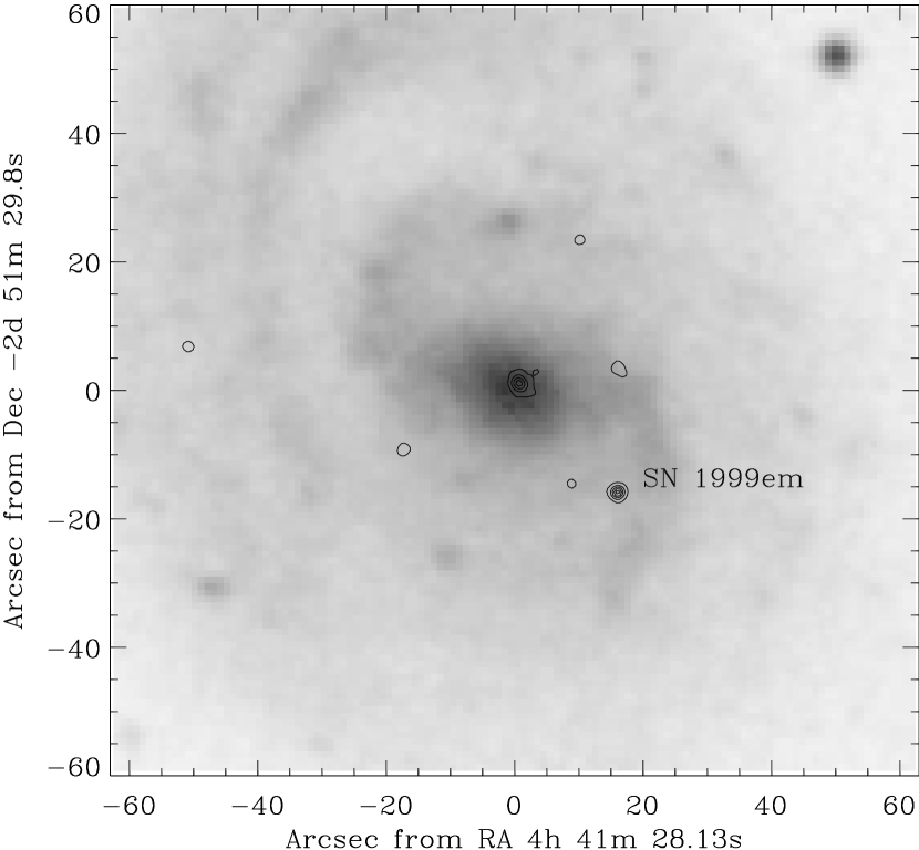
[th]

Figure 1: NGC 1637 in optical and X-rays. X-ray contours from the first Chandra observation of SN 1999em are overlaid on a DSS image of the host galaxy.

4 Results

4.1 SN 1999em

4.1.1 X-ray

The source was detected on all occasions, and an overlay of the X-ray contours from the first observation on an optical image of the host galaxy is shown in Fig. 1. The wavdetect position (based solely on the Chandra aspect solution) is 4^h41^m27$\fs$16, $-$2°51′45$\farcs$6, which is within 1″ (roughly the Chandra pointing accuracy) of the radio and optical positions. The low flux ($f_{\rm x}$ $\lesssim 10^{-14}$ ergs cm^-2 s^-1) resulted in few total counts (see Table 1). We have fit both the MEKAL and thermal Bremsstrahlung models to our data. The MEKAL model is a single-temperature, hot diffuse gas (Mewe, Gronenschild, & van den Oord, 1985) with elemental abundances set to the solar values of Anders & Grevesse (1989). We have calculated the column density (Predehl & Schmitt, 1995) to be $N_{\rm H}=6.1\times 10^{20}$ cm^-2 based upon a value of $E_{(B-V)}=0.05$ (Baron et al., 2000). For both models, only the temperatures and overall normalizations were allowed to vary. In XSPEC (Arnaud, 1996), we performed maximum likelihood fits on the unbinned data using Cash statistics (Cash, 1979). These fits should be insensitive to the number of counts per channel and are thus appropriate for fitting low-count data. The best-fit observed temperatures are shown in Table 3. As expected, the uncertainties in fit parameters for such low-count data are large.

We have also used flux ratios to characterize the source. The fluxes were calculated by manually integrating the source spectra, i.e., they are model-independent, absorbed fluxes. The first observation had a flux ratio of $f_{\rm x}$[2–8 keV]/$f_{\rm x}$[0.4–2 keV] $=2.1\pm 0.9$, but later observations were softer (Table 1). Somewhat surprisingly, the total flux nearly doubled from the third observation to the fourth, despite the continued decline of the high-energy X-rays. The multicolour X-ray lightcurve is shown in Fig. 2.

[!t]

Figure 2: X-ray and radio light curves of SN 1999em. The detections are shown with error bars while the upper limits are shown with downward arrows. Radio flux densities are plotted with the appropriate symbols. The absorbed X-ray flux is plotted in both the 2–8 keV (solid line) and 0.4–2 keV (dashed line) bands. The hard X-rays follow a steady decline, but the soft X-rays double from the third observation to the fourth.

4.1.2 Radio

After 15 unsuccessful VLA observations of SN 1999em at ages 4 to 19 days after the assumed explosion date of 1999 October 28, the SN was finally detected on day 34 with 0.190 mJy flux density at 8.435 GHz. Subsequent observing on days 46, 60, and 70 indicated that SN 1999em remained detectable at a similar flux density, near the sensitivity limit of the VLA, at 8.435, 4.885, and 1.465 GHz. The data are shown, together with the x-ray results, in Fig. 2. Since day 70, no radio detection of SN 1999em in any cm wavelength band has been obtained. SN 1999em is among only a few radio detected Type II-P, and its behavior is difficult to compare with other radio observations of the same type SN. An estimated spectral luminosity of SN 1999em at 6 cm peak on day $\sim$34 of $L_{\rm 6cm~{}peak}\sim 2.2\times 10^{25}$ erg s^-1 Hz^-1 makes it the least radio luminous RSN known except for the peculiar, and very nearby, SN 1987A. The radio position of the emission from SN 1999em is 4^h41^m27$\fs$157, $-$2°51′45$\farcs$83 (J2000). The details of the observations and analysis will be found in Lacey et al. (2002).

4.1.3 Optical

The spectropolarimetry of SN 1999em provided a rare opportunity to study the geometry of the electron-scattering atmosphere of a “normal” core-collapse event at multiple epochs (Leonard et al., 2001a). A very low but temporally increasing polarization level suggests a substantially spherical geometry at early times that becomes more aspherical at late times as ever-deeper layers of the ejecta are revealed. When modeled in terms of oblate, electron-scattering atmospheres, the observed polarization implies an asphericity of at least 7% during the period studied. We speculate that the thick hydrogen envelope intact at the time of explosion in SNe II-P might serve to dampen the effects of an intrinsically aspherical explosion. The increase in asphericity seen at later times is consistent with a trend recently identified (Wang et al., 2001) among stripped-envelope core-collapse SNe: the deeper we peer, the more evidence we find for asphericity. The natural conclusion that it is an explosion asymmetry that is responsible for the polarization has fueled the idea that some core-collapse SNe produce gamma-ray bursts (GRB; e.g., Bloom et al. 1999) through the action of a jet of material aimed fortuitously at the observer, the result of a “bipolar,” jet-induced, SN explosion (Khokhlov et al., 1999; Wheeler et al., 2000; Maeda et al., 2000). Additional multi-epoch spectropolarimetry of SNe II-P are clearly needed, however, to determine if the temporal polarization increase seen in SN 1999em is generic to this class.

4.2 SN 1998S

4.2.1 X-ray

The source was detected on all occasions, and an overlay of the X-ray contours from the first observation on an optical image of the host galaxy is shown in Fig. 3. The wavdetect position (based solely on the Chandra aspect solution) is 11^h46^m06$\fs$14, 47°28′55$\farcs$1 (J2000), which is within 0$\farcs$5 of the radio and optical positions. In addition to constructing multicolour X-ray lightcurves (Fig. 4), the high luminosity of SN 1998S ($\mbox{$L_{\rm x}$}\approx 10^{40}$ ergs s^-1) allowed for basic spectral fitting to be done for each of the first four observations; in the fifth, there were too few counts for a similar type of analysis. We performed this in XSPEC with the VMEKAL model, which is identical to the MEKAL model but allows individual elemental abundances to vary. Using the reddening $E_{(B-V)}=0.23$ (Leonard et al., 2000), we calculated the hydrogen column density to be $N_{\rm H}=1.36\times 10^{21}\ \mbox{cm${}^{-2}$}$ (Predehl & Schmitt, 1995). We used a redshift of $z=0.003$ (Willick et al., 1997).

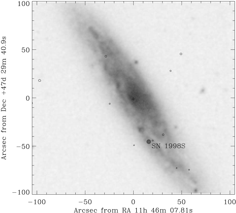
Figure 3: NGC 3877 in optical and X-rays. X-ray contours from the first Chandra observation of SN 1998S are overlaid on a DSS image of the host galaxy.

Figure 4: X-ray and radio light curves of SN 1998S. The detections are shown with error bars while the upper limits are shown with downward arrows. The absorbed X-ray flux declines in both the hard (solid lines) and soft (dashed lines) bands.

Although there were sufficient counts ($>$500 per observation) in each of the first four observations for spectral modeling, there were few counts per energy channel. To mitigate the problems associated with fitting such data, we grouped the data to contain a minimum number of counts per bin. Because there were virtually no counts above $\sim$ 7 keV in any of the observations, we would “smear” the Fe line at 6.7 keV if we required more than $\sim$ 7 counts per bin. Therefore, we set the minimum number of counts per bin to the highest possible value which would still retain the integrity of the Fe line. This turned out to be 5 counts per bin for the first observation, 7 for the second, 5 for the third, and 7 for the fourth.

To reduce the number of free parameters in our fits, we froze the abundance of He to its solar value. We also linked the abundances of N, Na, Al, Ar, and Ca to vary with C. The remaining elemental abundances (O, Ne, Mg, Si, S, Fe, and Ni) were allowed to vary independently. We first allowed the column density to vary in our fits. Since the best-fit results were all consistent with the $N_{\rm H}$ obtained from the optical reddening, we fixed this parameter at the calculated value.

Figure 5: Spectra of SN 1998S. The first observation is in the upper left, the second in the lower left, the third in the upper right, and the fourth in the lower right. Best-fit VMEKAL models are overplotted on evenly binned data.

We then performed $\chi^{2}$ fitting using Gehrels weighting for the statistical error (Gehrels, 1986), which is appropriate for low count data. We also performed maximum likelihood fits to the unbinned data using Cash statistics (Cash, 1979). The maximum likelihood fits were in good agreement with the $\chi^{2}$ fits, and we report the $\chi^{2}$ results in Table 4. We note, however, that fitting with so few counts per bin may give misleading $\chi^{2}$ values. For ease of viewing, we have plotted the best fit models against evenly binned data (Fig. 5).

In order to bring out the line features, we have summed the individual spectra. We feel justified in doing this because the best-fit model parameters from the four individual observations with enough counts for individual modeling are consistent with each other, indicating that the spectral shape is not changing much, only the overall normalization (luminosity). We grouped the summed spectrum to $\geq$15 counts per bin for spectral fitting. Grouping to more counts per bin than that would have washed out some of the weaker line features. The individual response functions for each observations were combined in a weighted average based on exposure times.

We fit four models to this summed spectrum: a single MEKAL plasma with solar abundances (1-T MEKAL); two MEKAL plasmas with solar abundances (2-T MEKAL); a single MEKAL plasma with variable abundances (all elements allowed to vary except He; 1-T VMEKAL); and a single MEKAL with solar abundances plus a single MEKAL with variable abundances (2-T VMEKAL). The 1-T MEKAL model did not fit the data well, with a $\chi^{2}$ of 181 for 124 degrees of freedom (dof). Tests of the other three model fits against this one using the F-statistic indicate that only the 1-T VMEKAL fit was a significant improvement (required at the 3.8 $\sigma$ level). Most of the abundances in this model are not well constrained (especially those of C, N, Na, and Ni). The uncertainty in each abundance was determined in the following way. The abundance was changed from the best-fit value, the model was refit (with all other parameters allowed to vary), and the resultant $\chi^{2}$ was compared to the best-fit $\chi^{2}$. This was repeated until the difference in $\chi^{2}$ was 2.706, which gave the 90% confidence interval for the given parameter. Table 5 lists the results. The best-fit temperature was $kT=9.8^{+2.2}_{-1.8}$ keV, and the fit statistic was $\chi^{2}=139$ for 116 degrees of freedom. Fig. 6 shows the summed spectrum and best-fit VMEKAL model with labels indicating the rough positions of elemental lines.

Figure 6: VMEKAL fit to the summed spectrum of SN 1998S. Labels indicate approximately where emission lines for each element would be observed.

4.2.2 Radio

Since its initial radio detection at 8.46 GHz on 1999 January 07 (310 days after optical discovery), SN 1998S has increased at all mid-cm wavelengths. Modeling indicates that it should reach its 6 cm flux density peak at age $\sim$1000 days, at roughly the epoch of the most recent observations on 2001 January 25. Assuming that is the case, SN 1998S is behaving like other radio-detected Type IIn (SNe 1986J and 1988Z both peaked at 6 cm wavelength at age $\sim$1000 days) although it will be the least radio luminous at 6 cm peak ($L_{\rm 6cm~{}peak}\sim 3.6\times 10^{26}$ erg s^-1 Hz^-1) of the six Type IIn RSNe known (SNe 1978K, 1986J, 1988Z, 1995N, 1997eg, and 1998S). The radio data are shown together with the X-ray results in Fig. 4.

Under the Chevalier model of a dense CSM established by a slow pre-supernova stellar wind ($v_{w}$ = 10 km s^-1, $v_{\rm shock}=10^{4}$ km s^-1, $T=2\times 10^{4}$ K; see, e.g., Weiler et al. 1986), such a radio luminosity is interpreted as indicative of a mass-loss rate of $\sim 2\times 10^{-4}$ M_⊙ yr^-1. The radio position of the emission from SN 1998S is 11^h46^m6$\fs$140, 47°28′55$\farcs$45. The details of the observations and analysis will be found in Lacey et al. (2002). It should be noted that the best fit to the radio data requires significant clumping or filamentation in the CSM, as was also found for the Type IIn SNe 1986J and 1988Z (Weiler et al., 1990; Van Dyk et al., 1993).

4.2.3 Optical

SN 1998S exhibits a high degree of linear polarization, implying significant asphericity for its continuum-scattering environment (Leonard et al., 2000). Prior to removal of the interstellar polarization, the polarization spectrum is characterized by a flat continuum (at $p\approx 2\%$) with distinct changes in polarization associated with both the broad (symmetric, half width near zero intensity $\gtrsim 10,000$ km s^-1) and narrow (unresolved, full width at half maximum $<300$ km s^-1) line emission seen in the total flux spectrum. When analyzed in terms of a polarized continuum with unpolarized broad-line recombination emission, an intrinsic continuum polarization of $p\approx 3\%$ results, suggesting a global asphericity of $\gtrsim 45\%$ from the oblate, electron-scattering dominated models of Höflich (1991). The smooth, blue continuum evident at early times is inconsistent with a reddened, single-temperature blackbody, instead having a color temperature that increases with decreasing wavelength. Broad emission-line profiles with distinct blue and red peaks are seen in the total flux spectra at later times, suggesting a disk-like or ring-like morphology for the dense ($n_{e}\approx 10^{7}{\rm\ cm^{-3}}$) circumstellar medium, generically similar to what is seen directly in SN 1987A, although much denser and closer to the progenitor in SN 1998S. Such a disk/ring-like circumstellar medium may have formed from a merging of a binary-companion star that ejects the common-envelope material in the direction of the orbital plane of the binary system (Nomoto, Iwamoto, & Suzuki, 1995).

5 Discussion

5.1 SN 1999em

To interpret the X-ray and radio data on SN 1999em, we use the circumstellar interaction model proposed by Chevalier (1982), and elaborated by Chevalier & Fransson (1994) and Fransson, Lundqvist, & Chevalier (1996; hereafter, FLC96). The outer supernova ejecta are taken to be freely expanding, with a power law density profile

$$\rho_{sn}=At^{-3}(r/t)^{-n},$$ (1)

where $A$ and $n$ are constants. SN 1999em was a Type II-P SN, so we expect that the star exploded as a red supergiant with most of its hydrogen envelope. The value of $n$ for such a star is usually taken to be in the range $7-12$ (Chevalier, 1982), although Matzner & McKee (1999) recently found that the explosion of a red supergiant leads to $n=11.9$ at high velocity. In the case of SN 1999em, we have some additional information from modeling of the optical spectrum. Baron et al. (2000) were able to model spectra on 1999 October 29 and November 4/5 with $n=7$, 8, or 9. The modeling of the data for the earlier time suggests a relatively flat density profile ($n=7$). The spectra on 1999 October 29 also show evidence for a secondary absorption feature at 20,000 km s^-1, implying the presence of denser material in the cool ejecta. One possible origin for high velocity, dense ejecta is the shell that can form as a result of the diffusion of radiation at the time of shock breakout (Chevalier 1976); if this is the origin, it represents the highest velocity material in the ejecta. We assume that the outer density profile can be approximated as a power law out to this high velocity and take $n=7$ or $9$. The value of $A$ is equivalent to specifying the density in the ejecta at some particular velocity and age. The model by Baron et al. (2000) for 1999 October 29 has $\rho_{sn}=0.4\times 10^{-20}$ g cm^-3 at 10,000 km s^-1 at an age of 1 year. This value is in approximate accord with the density found in models with a broken power law density profile, mass of 10 M_⊙, and energy of $1\times 10^{51}$ ergs (Chevalier & Fransson, 1994).

The density in the wind is $\rho_{w}=\dot{M}/(4\pi r^{2}v_{w})$, where $\dot{M}$ is the mass-loss rate and $v_{w}$ is the wind velocity. We take $\dot{M}_{-6}=\dot{M}/10^{-6}$ M_⊙ yr^-1 and $v_{w1}=v_{w}/10$ km s^-1 as reference values. The interaction of the supernova with a freely expanding wind leads to a shocked shell with radius $R\propto t^{0.8}(n=7)$ or $t^{6/7}(n=9)$. This shell is the source of the X-ray emission. The low observed X-ray luminosity suggests that the shocked gas is not radiative; this can be checked for consistency after a model is produced. Under these conditions, the X-ray luminosity is expected to be dominated by emission from the reverse shock region, which is relatively cool, as observed. The luminosity of the shell can be estimated from eq. (3.10) of FLC96

$$L_{rev}=2.0\times 10^{35}\zeta(n-3)(n-4)^{2}T_{8}^{-0.24}e^{-0.116/T_{8}}\left(\dot{M}_{-6}\over v_{w1}\right)^{2}V_{4}^{-1}\left(t\over 10{\rm~{}days}\right)^{-1}{\rm~{}ergs~{}s^{-1}~{}keV^{-1}},$$ (2)

where $\zeta$ is 0.86 for solar abundances and 0.60 for $n({\rm He})/n({\rm H})=1$, $T_{8}=T/10^{8}$ K, and $V_{4}$ is the peak velocity in units of $10^{4}$ km s^-1. Baron et al. (2000) find possible evidence for enhanced He in SN 1999em, but this is uncertain and is probably not expected in a Type II-P SN. We take $\zeta=0.86$; the uncertainty is small. On 1999 November 1, which we take to be day 4, the observed luminosity (0.4–8 keV) is $2\times 10^{38}$ ergs s^-1 and the temperature is 5.0 keV. With $V_{4}=1.5$, we find that $\dot{M}_{-6}/v_{w1}\approx 1$ $(n=9)$ or 2 $(n=7)$, quite similar to the value of $\dot{M}_{-6}/v_{w1}\sim 2$ obtained above from the radio observations. With this mass-loss rate, the cooling time for the gas, as deduced from eq. (3.7) of FLC96, is $31$ days for $n=9$ and is longer for the $n=7$ case, which justifies our use of the adiabatic expression for the X-ray luminosity. The cooling time grows more rapidly than the age, so we expect non-radiative evolution through the time of our observations. If cooling were important, a dense shell would form that could absorb X-ray emission from the reverse shock wave, as appeared to occur in the initial evolution of SN 1993J (FLC96; Suzuki & Nomoto 1995). Reradiation of the absorbed emission can give broad optical emission lines, as observed in SN 1993J at ages $\gtrsim 1$ year. Such lines were not observed in SN 1999em, which is consistent with non-radiative evolution.

From eq. (2.2) of FLC96 with $n=9$, we find that the maximum velocity for $n=9$ is

$$V=\left(4\pi\rho_{o}t_{o}^{3}v_{o}^{9}v_{w}\over 15\dot{M}\right)^{1/7}t^{-1/7},$$ (3)

where $\rho_{o}$ specifies an ejecta density at a particular time $t_{o}$ and velocity $v_{o}$, as described above. At $t=4$ days with $\rho_{o}=0.4\times 10^{-20}$ g cm^-3 at $v_{o}=10,000$ km s^-1 and $t_{o}=1$ year and $\dot{M}_{-6}/v_{w1}=1$, we have $V=13,000$ km s^-1. For the $n=7$ case with $\dot{M}_{-6}/v_{w1}=2$, we have $V=14,000$ km s^-1 and $V\propto t^{-0.2}$. These velocities are lower than the highest velocities deduced by Baron et al. (2000) on 1999 October 29 (day 1). However, there is some uncertainty in the high velocity, and there may have been rapid evolution at early times.

The shock velocity determines the temperature of the reverse shock region. From eqs. (3.1) and (3.2) of FLC96, we have $T_{\rm rev}=2.4V_{4}^{2}$ keV for $n=9$, so that with $V_{4}=1.3$, $T_{\rm rev}=4.1$ keV. For $n=7$, we have $T_{\rm rev}=4.8V_{4}^{2}$ keV so $T_{\rm rev}=9.4$ keV for $V_{4}=1.4$. The observed temperature on 1999 November 1 falls between these two cases. The predicted evolution of the temperature is $T\propto V^{2}\propto t^{-2/(n-2)}\propto t^{-2/7}$ $(n=9)$ and $\propto t^{-0.4}$ $(n=7)$. Table 3 compares this predicted evolution with that observed. The observations show a clear cooling, as expected. An additional factor could be the lack of electron-ion equilibration at the reverse shock front; if it is not achieved, the electrons are cooler than the above estimate. From eq. (3.6) of FLC96, the expected conditions are such that the equilibration timescale is comparable to the age throughout the evolution, so that no firm conclusion can be drawn. The fact that cooling of the emission is clearly observed argues for a relatively flat density profile for the ejecta, as also found by Baron et al. (2000) from optical spectroscopy.

An estimate of the expected evolution of the total X-ray luminosity, $L_{\rm x}$, is given by Chevalier & Fransson (1994). When free-free emission dominates ($T\geq 4\times 10^{7}$ K), $\mbox{$L_{\rm x}$}\propto t^{-1}$, and when lines dominate ($10^{5}\leq T<4\times 10^{7}$ K), $\mbox{$L_{\rm x}$}\propto t^{-0.69}$ $(n=9)$ or $\propto t^{-0.56}$ $(n=7)$. The observed evolution is less steep than $t^{-1}$ and is closer to the expectation for line emission. The observed temperatures indicate that a transition occurred. Again, the observations are in approximate accord with expectations.

One aspect of the X-ray observations that is not compatible with the simplest wind interaction model is the increase of the soft X-ray flux on 2000 February 2 (day 102, see Fig. 2). In our model, the emission is primarily from the reverse shocked ejecta, so the increase could be due to a region of increased density in the ejecta. At this age, the velocity of the ejecta entering the reverse shock front is $\sim 8,000$ km s^-1. Alternatively, the emission could be from an inhomogeneity in the circumstellar wind. The smooth wind is shocked to a temperature $\sim 10^{9}$ K, so that a density contrast of $\sim 100$ is needed for the inhomogeneity. The inhomogeneity must be large to affect the total luminosity, but a substantial change in stellar mass-loss characteristics at only $10^{16}$ cm from the star is unlikely. The fact that the change is transitory also argues against a change in mass-loss properties at this point.

Although SN 1999em was detected as a weak radio source, the radio light curves are not well defined because of the very low radio flux density. The early observations were not of sufficient sensitivity to detect the source so the time of light curve peak and the early absorption process are also not well defined. The 8.44 GHz observations are the most useful in this regard. At late times, the observed flux evolution of other radio supernovae is $\propto t^{-0.7}$, or steeper (Weiler et al., 1986), so that the 8.44 GHz upper limit on day 7 probably indicates that absorption was significant at that time. With this value for the time of peak flux at 8.44 GHz (actually a lower limit), we can place SN 1999em on a diagram of peak radio luminosity vs. time of peak (Fig. 7). The diagonal lines show the velocity of the shocked shell if synchrotron self-absorption were the important process for the early absorption (Chevalier, 1998). The position of SN 1999em gives about $10,000$ km s^-1, or less, as the shell velocity. Thus, it is just possible that synchrotron self-absorption was important at early times but more likely that another process, probably free-free absorption by the unshocked wind, was dominant. From eq. (2.3) of FLC96, the 8.44 GHz free-free optical depth on day 7 with $V_{4}$ and $\dot{M}_{-6}/v_{w1}$ as deduced above is $\tau=0.2T_{5}^{-3/2}$ $(n=9)$ or $0.5T_{5}^{-3/2}$ $(n=7)$, where $T_{5}$ is the temperature of the unshocked wind in units of $10^{5}$ K. The $n=7$ case is somewhat more consistent with the observations because of the higher mass-loss rate deduced for this case.

Figure 7: The peak spectral radio luminosity vs the product of the time of the peak and the frequency of the measurement, based on Fig. 4 of Chevalier (1998) with the addition of SN 1998bw, SN 1998S, and SN 1999em. The observed supernovae are designated by the last two digits of the year and the letter, and are of Types II (stars), Ib (squares), and Ic (crosses). The dashed lines show the mean velocity of the radio shell if synchrotron self-absorption is responsible for determining the flux density peak; an electron spectrum $N(E)\propto E^{-2.5}$ is assumed.

The free-free absorption of the radio emission depends on the circumstellar temperature. Eastman et al. (1994) find from a simulation of a Type II-P explosion an effective temperature at outbreak of $T_{\rm eff}=1.8\times 10^{5}$ K and luminosity $9\times 10^{44}$ ergs s^-1. This temperature is similar to that used in one model by Lundqvist & Fransson (1991) for SN 1987A (their Table 1). Their model with $\dot{M}_{-6}/v_{w1}=0.4$ gives a wind temperature of $1.2\times 10^{5}$ K for $T_{\rm eff}=2\times 10^{5}$ K. Because of the low wind density, this temperature is not sensitive to the mass-loss rate and is mainly set by the outburst radiation temperature. An approximate temperature in the wind of SN 1999em should therefore be $T_{5}\approx 1.2$. The temperature at $\sim$30 days should not be very different because of the low wind density. X-ray heating by the shock has not been included here, but is probably not important because of the low X-ray luminosity.

Overall, the X-ray and radio observations of SN 1999em are consistent with the non-radiative interaction of supernova ejecta with a power law profile ($n\sim 7$) interacting with a pre-supernova wind with $\dot{M}_{-6}/v_{w1}\approx 2$. We estimate the accuracy of this mass-loss density to be a factor of 2. The X-ray emission is primarily from the reversed shocked ejecta, and the model can account for the luminosity, temperature, and temperature evolution of the emission. It does not account for the large soft X-ray flux observed on day 102. The radio observations are compatible with this general picture and suggest a comparable mass-loss rate.

5.2 SN 1998S

The high X-ray luminosity of SN 1998S places it in the same class as the X-ray bright Type IIn SNe 1978K, 1986J, 1988Z, and 1995N. Fox et al. (2000) discussed X-ray observations of SN 1995N and summarized the results on the other SNe. SN 1995N had an X-ray luminosity of $1.5\times 10^{41}$ ergs s^-1 at an age of 2.0 years. SN 1998S is at the low end of the X-ray luminosities spanned by these sources

The optical emission from SN 1998S shows both narrow and broad lines that can be attributed to circumstellar interaction (Fassia et al., 2000; Leonard et al., 2000; Chugai, 2001). The narrow lines are presumably from dense circumstellar gas that is heated and ionized by the supernova radiation. Although high velocities ($V_{4}\approx 1$) are observed in the early evolution of SN 1998S, by day 494 the maximum observed velocities were $V_{4}=0.5-0.6$ (Leonard et al., 2000). These velocities are much higher than the estimated velocity of gas at the photosphere, indicating that the emission is from circumstellar interaction.

The interpretation of the X-ray emission from Type IIn supernovae is not straightforward because of the possibility that the emission is from shocked circumstellar clumps (see, e.g., Weiler et al. 1990 and Chugai 1993 on SN 1986J and Van Dyk et al. 1993 on SN 1988Z). The radio results for SN 1998S indicate that the CSM is likely clumpy or filamentary (Lacey et al., 2002). However, if our finding of heavy element overabundances is correct, the X-ray emission is expected to be from shocked SN ejecta. If the interaction can be approximately described by smooth ejecta running into a smooth circumstellar wind, the temperature behind the reverse shock front is $T_{\rm rev}=2.4V_{4}^{2}$ keV ($n=9$), $5.4V_{4}^{2}$ keV ($n=7$), or $9.6V_{4}^{2}$ keV ($n=6$). It is difficult to produce the high observed temperature ($T\approx 10$ keV) unless there is unseen high velocity gas and the ejecta density profile is relatively flat. The observations do not show the cooling that is expected as the shock interaction region decelerates, but the range in time is not large enough for the effect to be clearly visible.

The X-ray luminosity shows a clear decline with time, approximately $\propto t^{-1.3}$. This is in reasonable agreement with what is expected for free-free emission from a non-radiative shock region ($t^{-1}$ dependence as discussed above), so we can again use eq. (2) to estimate the mass-loss rate. The result is $\dot{M}_{-4}/v_{w1}=(1-2)$, where $\dot{M}_{-4}=\dot{M}/10^{-4}$ M_⊙ yr^-1, if $n=6$ and $V_{4}=1$ (these estimates are implied by the high observed temperature of $\sim$10 keV) on day 665, again comparable to that determined from radio modeling of $\dot{M}_{-4}/v_{w1}\sim 2$. A high mass-loss rate is required to produce the X-ray luminosity, but the cooling time is still longer than the age. The assumption of a non-radiative reverse shock region is justified. In this model, the X-ray luminosity of the forward shock region is comparable to that from the reverse shock. However, the higher temperature of the forward shock region implies that the reverse shock dominates the emission in the energy band that we observed.

The radio luminosity of SN 1998S is low for a RSN with a late turn-on time (see Fig. 7). This implies that synchrotron self-absorption was not important for the early absorption. This accounts for the basic features of the X-ray emission. The flat supernova density profile implies that much of the supernova energy is in high velocity ejecta. A similar deduction was made by Chugai & Danziger (1994) for SN 1988Z. The heavy element overabundances require that these elements be mixed out to a high velocity in the ejecta, which has been shown to occur in Cas A (Hughes et al., 2000). In theoretical models of aspherical explosions, heavy-element-rich matter is naturally ejected at high velocities, which well explains the peculiar late spectral features of SN 1998bw (Maeda et al., 2000). The polarization and spectral line profiles observed in SN 1998S (Leonard et al., 2000) show that the explosion was complex, i.e. that the spherically symmetric model described here must be an oversimplification.

We turn now to the observed elemental abundance ratios in the summed Chandra spectrum (Table 5), which are enhanced by a factor of $\sim$ 3 - 30 over solar. These heavy elements must have been synthesized in the core evolution and explosion.

In core-collapse supernovae, a strong shock wave forms and propagates outward through the star (e.g., Shigeyama & Nomoto 1990). Behind the shock, materials are explosively burned into heavy elements and accelerated to $\sim$5000 km s^-1. At the composition interface, the expanding materials are decelerated by the collision with the outer layers, which induces the Rayleigh-Taylor instability (e.g., Ebisuzaki, Nomoto, & Nomoto 1988; Arnett et al. 1989). Heavy elements are then mixed into outer layers. Such a mixing induced at the Si/O, C/He, and He/H interfaces brings Fe-peak elements, as well as Si, Mg, Ne, O, and C, into the H-rich envelope. These heavy elements in many Rayleigh-Taylor fingers are rather well-mixed through the interaction between the fingers (e.g., Hachisu et al. 1992). We thus assume that, although the heavy elements mixed into the H-rich envelope consists of only a fraction of the core materials, the abundance ratios among the mixed heavy elements are the same as in the integrated core materials. The mixing associated with the Rayleigh-Taylor instabilities continues until the shock wave reaches the surface and the expansion becomes homologous.

When the ejecta collides with the circumstellar matter, forward and reverse shock waves form and the latter propagates back into the H-rich envelope. The mass of the reverse-shocked H-rich envelope $\delta M_{\rm H}$ at the time of the observations depends on the strength of the circumstellar interaction and the density structure of the H-rich envelope (e.g., Chevalier & Fransson 1994; Suzuki & Nomoto 1995). We denote by $\delta M_{\rm Z}$ the mass of heavy elements mixed into the reverse-shocked H-rich envelope. The observed mass fraction of heavy elements is then $\delta M_{\rm Z}$/$X\delta M_{\rm H}$, where $X$ denotes the H mass fraction.

We briefly summarize here the three types of heavy elements ejected from core-collapse SNe (e.g., Thielemann, Nomoto, & Hashimoto 1996):

O, Ne, and Mg:

These elements are synthesized mostly before collapse during core- and shell-C burning; some Ne is processed into Mg and O during Ne burning. In the explosion, these elements are partially produced by explosive C burning, Ne is partially burned into Mg and Si, and O and Mg are partially burned into Si. The masses of these elements are sensitive to the progenitor mass, $M$, increasing with $M$. However, the degree of dependence on $M$ varies across elements. For example, the Ne/Mg ratio depends on the conditions of C and Ne burning, thus depending on $M$.

Si, S, and Ar:

These elements are produced by explosive O burning during the explosion. Their masses do not much depend on $M$ since the pre-collapse core structure is not very sensitive to $M$.

Fe:

The mass of ejected Fe is very sensitive to the mass cut that divides the compact remnant and the ejecta, or the amount of fall-back matter. Theoretically, it is not possible to make a good estimate of the Fe mass because of the uncertainties in the explosion mechanism.

In our comparisons, we use Si for normalization because it is the least dependent on $M$. We do not use Fe for comparison because of the large theoretical uncertainties. We now compare the O/Si, Ne/Si, and Mg/Si ratios (relative to the solar abundance ratios) with the theoretical calculations of Nomoto et al. (1997). These models are summarized in Table 6.

The observed O/Si value of 0–1.2 seems to indicate that the mass of the progenitor was $\lesssim$20 M_⊙. The Mg/Si value of 0–0.7 also points to a progenitor mass of $<$20 M_⊙. The observed Ne/Si ratio of 0.6–14 excludes progenitor masses of $\lesssim$15 M_⊙. According to these models, the mass of the proginitor must have been between 15 M_⊙ and 20 M_⊙.

We note that the supernova yields are determined by the helium core mass $M_{\rm He}$ of the progenitor rather than the zero-age main-sequence mass $M$. Thus the Mg/Si and Ne/Si results actually provide the constraint $M_{\rm He}=5\pm 1~{}\mbox{M${}_{\odot}$}$ (Nomoto et al., 1997). The $M$-$M_{\rm He}$ relation depends on the mass loss. If we adopt the spiral-in binary scenario for the origin of Type IIn SN (Nomoto, Iwamoto, & Suzuki, 1995), a large amount of mass-loss in the early phase of the progenitor’s expansion leads to a smaller $M_{\rm He}$ compared with the case of no mass loss. In this case, the progenitor of SN 1998S could be initially more massive.

6 Summary

Observations at radio, optical, and X-ray wavelengths have allowed the estimation of the physical parameters of two quite different Type II SN examples, Type II-P SN 1999em and Type IIn SN 1998S. From these results, it is possible to study, over a broad wavelength range, the physical parameters of the explosions and the structure and density of the CSM established by the pre-SN wind. Such results are of importance for estimation of the properties of the pre-SN star and its last stages of evolution before explosion (e.g., Nomoto, Iwamoto, & Suzuki 1995). In addition, the Chandra data have revealed the presence of many heavy elements in the spectrum of SN 1998S. We have shown the kind of analysis that can be done by comparing the observed X-ray determined abundance ratios to the model predictions, and we were able to show that the mass of the progenitor was $\sim$15–20 M_⊙. We do caution, however, that our model assumptions on mixing are approximate and that there are uncertainties in both the interpretation of the X-ray data and the model calculations. Because of the great diversity of Type II (and related Type Ib/c) SNe, only the multiwavelength study of additional examples can yield a comprehensive understanding of the last stages of massive star evolution.

7 Acknowledgments

DP acknowledges that this material is based upon work supported under a National Science Foundation Graduate Fellowship. WHGL and RAC gratefully acknowledge support from NASA. RAC is grateful to E. Baron for useful correspondence. KWW wishes to thank the Office of Naval Research (ONR) for the 6.1 funding supporting this research. Additional information and data on radio emission from SNe can be found on http://rsd-www.nrl.navy.mil/7214/weiler/ and linked pages. AVF is grateful for the support of NASA/ Chandra grants GO0-1001C and GO1-2062D. KN has been supported in part by the Grant-in-Aid for COE Scientific Research (07CE2002, 12640233) of the Ministry of Education, Science, Culture, and Sports in Japan.

Table 1: Chandra Observations of SN 1999em.

Date	Day	Length	Length After Filtering	Count Rate	$f_{\rm x}$[2–10 keV]/
	(From Ref.)	(ksec)	(ksec)	(cts ksec-1)	$f_{\rm x}$[0.4–2 keV]
1999 Nov 1	4	29.0	21.6	3.70	$2.1\pm 0.9$
1999 Nov 13	16	26.0	10.6	2.46	$0.8\pm 0.4$
1999 Dec 16	49	35.3	35.1	1.02	$0.7\pm 0.5$
2000 Feb 7	102	38.5	23.9	1.84	$0.2\pm 0.1$
2000 Oct 30	368	26.4	26.4	0.46	$0.9\pm 0.5$
2001 Mar 9	495	26.7	24.6	0.31	$0$
2001 Jul 22	630	29.8	25.1	0.19	$0$

Table 2: Chandra Observations of SN 1998S.

Date	Day	Length	Length After Filtering	Count Rate
	(From Ref.)	(ksec)	(ksec)	(cts ksec-1)
2000 Jan 10	678	18.9	18.9	34.4
2000 Mar 7	735	23.4	23.1	30.3
2000 Aug 1	882	19.8	19.8	25.8
2001 Jan 14	1048	29.2	29.2	19.5
2001 Oct 17	1324	28.7	14.8	12.4

Table 3: X-ray Temperature Evolution of SN 1999em.

Day	Obs. MEKAL $kT$	Obs. Brems. $kT$	Model $kT$ ($n=7$)	Model $kT$ ($n=9$)
(From Ref.)	(keV)	(keV)	(keV)	(keV)
4	$5.0^{+5.1}_{-2.1}$	$5.2^{+11.5}_{-2.3}$	9.2	4.1
16	$2.5^{+2.7}_{-0.9}$	$2.3^{+5.9}_{-1.1}$	5.4	2.8
49	$2.9^{+2.6}_{-1.1}$	$2.2^{+3.2}_{-0.9}$	3.4	2.0
102	$0.8^{+0.2}_{-0.1}$	$1.1^{+0.7}_{-0.4}$	2.5	1.6
368	$1.0^{+0.7}_{-0.3}$	$1.5^{+6.5}_{-0.8}$	1.5	1.1

Note. — Listed uncertainties are 90% confidence intervals.

Table 4: VMEKAL Fits to the Spectra of SN 1998S.

Day	$kT$	Fe Abund.	$\chi^{2}$/d.o.f.	$L_{\rm x}$[2–10 keV]
(From Ref.)	(keV)	(w.r.t. solar)		(ergs s-1)
678	$10.4_{-2.2}^{+81.9}$	$6.5_{-6.5}^{+63}$	82.7/96	$9.3\times 10^{39}$
735	$9.6_{-2.2}^{+5.5}$	$4.2_{-2.6}^{+7.3}$	71.7/71	$8.8\times 10^{39}$
882	$10.4_{-4.2}^{+14.1}$	$2.8_{-2.8}^{+15.8}$	65.8/75	$6.1\times 10^{39}$
1048	$8.0_{-2.1}^{+3.7}$	$5.4_{-3.5}^{+14.5}$	57.0/59	$5.3\times 10^{39}$

Note. — Listed uncertainties are 90% confidence intervals.

Table 5: Elemental Abundances from VMEKAL Fit to Summed Spectrum of SN 1998S.

Element	Best-fit Abund.	90% Confidence Interval
O	0.7	0–2.9
Ne	15	8.7–35
Mg	0	0–1.6
Al	33	0–135
Si	5.7	2.4–15
S	8.7	3.0–24
Ar	18	3.4–52
Ca	0.8	0–13
Fe	3.0	1.8–6.8
C	1.0	0–200
N	0	0–18
Na	0	0–36
Ni	0	0–14

Note. — These abundances are actually the ratio of a given element to H normalized to the similar solar ratio. For example, “Ne” is actually [(Ne/H)_98S]/[(Ne/H)_⊙].

Table 6: Elemental Abundance Ratios Relative to Solar for SN 1998S and Theoretical Models.

Abund. ratio	SN 1998S	13 M⊙	15 M⊙	18 M⊙	20 M⊙	25 M⊙	40 M⊙
Ne/Si	0.6–14	0.14	0.17	0.86	1.1	2.2	0.56
Mg/Si	0–0.7	0.18	0.49	0.58	1.09	2.1	1.1
O/Si	0–1.2	0.20	0.43	0.80	1.4	2.4	1.6

References

- Anders & Grevesse (1989) Anders, E., & Grevesse, N. 1989, Geochim. Cosmochim. Acta, 53 197
- Arnaud (1996) Arnaud, K. 1996, in Jacoby, G., & Branes, J., eds, ASP Conf. Ser. Vol. 101, Astronomical Data Analysis Software and Systems V, Astron. Soc. Pac., San Francisco
- Arnet et al. (1989) Arnett, W. D., Bahcall, J. N., Kirshner, R., & Woosley, S. E. 1989, ARA&A, 27, 629
- Baron et al. (2000) Baron, E., Branch, D., Hauschildt, P. H., Filippenko, A. V., Kirshner, R. P., Challis, P. M., Jha, S., Chevalier, R. A., Fransson, C., Lundqvist, P., Garnavich, P., Leibundgut, B., McCray, R., Michael, E., Panagia, N., Phillips, M. M., Pun, C. S. J., Schmidt, B., Sonneborn, G., Suntzeff, N. B., Wang, L., & Wheeler, J. C. 2000, ApJ, 545, 444
- Bloom et al. (1999) Bloom, J. S., Kulkarni, S. R., Djorgovski, S. G., Eichelberger, A. C., Cote, P., Blakeslee, J. P., Odewahn, S. C., Harrison, F. A., Frail, D. A., Filippenko, A. V., Leonard, D. C., Riess, A. G., Spinrad, H., Stern, D., Bunker, A., Dey, A., Grossan, B., Perlmutter, S., Knop, R. A., Hook, I. M., & Feroci, M. 1999, Nature, 401, 453
- Branch et al. (1981) Branch, D., Falk, S. W., McCall, M. L., Rybski, P., Uomoto, A. K., & Wills, B. J. 1981, ApJ, 244, 780
- Bregman & Pildis (1992) Bregman, J. N.,& Pildis, R. A. 1992, ApJ, 398, L107
- Burrows et al. (2000) Burrows, D., Michael, E., Hwang, R., McCray, R., Chevalier, R., Petre, R., Garmire, G., Gordon, P., Holt, S., Nousek, J. 2000, ApJ, 543, L149
- Canizares, Kriss, & Feigelson (1982) Canizares, C. R., Kriss, G. A., & Feigelson, E. D. 1982, ApJ, 253, L17
- Cash (1979) Cash, W. 1979, ApJ, 228, 939
- Chevalier (1976) Chevalier, R. A. 1976, ApJ 207, 872
- Chevalier (1982) Chevalier, R. A. 1982, ApJ, 259, 302
- Chevalier & Fransson (1994) Chevalier, R. A., & Fransson, C. 1994, ApJ, 420, 268
- Chevalier (1998) Chevalier, R. A. 1998, ApJ, 499, 810
- Chugai (2001) Chugai, N. N. 2001, MNRAS, submitted (astro-ph/0106234)
- Chugai (1993) Chugai, N. N. 1993, ApJ, 414, L101
- Chugai & Danziger (1994) Chugai, N. N., & Danziger, I. J. 1994, MNRAS, 268, 173
- LRISp; Cohen (1996) Cohen, M. H. 1996, The LRIS Polarimeter (Keck Obs. Instrument Manual), http://www2.keck.hawaii.edu:3636/
- Eastman et al. (1994) Eastman, R. G., Woosley, S. E., Weaver, T. A., & Pinto, P. A. 1994, ApJ, 430, 300
- Dennerl et al. (2001) Dennerl, K., et al., 2001, A&A, 365, L202
- Ebisuzaki, Shigeyama, & Nomoto (1989) Ebisuzaki, T., Shigeyama, T., & Nomoto, K. 1989, ApJ, 344, L65
- Fabian & Terlevich (1996) Fabian, A. C.,& Terlevich, R. 1996, MNRAS, 280, L5
- Fassia et al. (2000) Fassia, A., Meikle, W. P. S., Vacca, W. D., Kemp, S. N., Walton, N. A., Pollacco, D. L., Smartt, S., Oscoz, A., Aragón-Salamanca, A., Bennett, S., Hawarden, T. G., Alonso, A., Alcalde, D., Pedrosa, A., Telting, J., Arevalo, M. J., Deeg, H. J., Garzón, F., Gómez-Roldán, A., Gómez, G., Gutiérrez, C., López, S., Rozas, M., Serra-Ricart, M., & Zapatero-Osorio, M. R. 2000, MNRAS, 318, 1093
- Fesen & Becker (1990) Fesen, R. A., & Becker, R. H. 1990, ApJ, 351, 437
- Fesen & Matonick (1993) Fesen, R. A., & Matonick, D. M. 1993, ApJ, 407, 110
- Filippenko & Barth (1997) Filippenko, A. V., & Barth, A. J. 1997, IAU Circ., 6794
- Filippenko (1997) Filippenko, A. V. 1997, ARA&A, 35, 309
- Filippenko & Moran (1998) Filippenko, A. V., & Moran, E. C. 1998, IAU Circ., 6830
- Filippenko et al. (2001) Filippenko, A. V., et al. 2001, in preparation
- Fox et al. (1999) Fox, D. W., & Lewin, W. H. G. 1999, IAU Circ., 7318
- Fox et al. (2000) Fox, D. W., Lewin, W. H. G., Fabian, A., Iwasawa, K., Terlevich, R., Zimmermann, H. U., Aschenbach, B., Weiler, K., Van Dyk, S., Chevalier, R., Rutledge, R., Inoue, H., & Uno, S. 2000, MNRAS, 319, 1154
- Fransson, Lundqvist, & Chevalier (1996; hereafter, FLC96) Fransson, C., Lundqvist, P., & Chevalier, R. A. 1996, ApJ, 461, 993, (FLC96)
- Fransson & Björnsson (1998) Fransson, C., & Björnsson, C.-I. 1998, ApJ, 509, 861
- Garnavich, Jha, & Kirshner (1998a) Garnavich, P., Jha, S., & Kirshner, R. 1998a, IAU Circ., 6832
- Garnavich et al. (1998b) Garnavich, P., Kirshner, R., Challis, P., Koranyi, D., & Culkins, M. 1998b, IAU Circ., 6845
- Gehrels (1986) Gehrels, N. 1986, ApJ, 303, 336
- Gorenstein, Hughes, & Tucker (1994) Gorenstein, P., Hughes, J. P., Tucker, W. H., ApJ, 420, L25
- Granslo et al. (1998) Granslo, B. H., Shanklin, J., Carvajal, J., & Hornoch, K. 1998, IAU Circ., 6846
- Hachisu et al. (1992) Hachisu, I., Matsuda, T., Nomoto, K., & Shigeyama, T. 1992, ApJ, 390, 230
- Hamuy et al. (2001) Hamuy, M., et al. 2001, ApJ, in press (astro-ph/0105006)
- Hasinger, Aschenbach, & Trüumper (1996) Hasinger, G., Aschenbach, B., & Trüumper, J. 1996, A&A, 312, L9
- Höflich (1991) Höflich, P. 1991, A&A, 246, 418
- Houck et al. (1998) Houck, J. C., Bregman, J. N., Chevalier, R. A., & Tomisaka, K. 1998, ApJ, 493, 431
- Hughes et al. (2000) Hughes, J. P., Rakowski, C. E., Burrows, D. N., & Slane, P. O. 2000, ApJ, 528, L109
- Immler, Pietsch, & Aschenbach (1998a) Immler, S., Pietsch, W., & Aschenbach, B. 1998a, A&A, 331, 601
- Immler, Pietsch, & Aschenbach (1998b) Immler, S., Pietsch, W., & Aschenbach, B. 1998b, A&A, 336, L1
- Immler, Aschenbach, & Wang (2001) Immler, S., Aschenbach, B., Wang, Q. D. 2001, ApJ, 561, L107
- Immler, Wilson, & Terashima (2002) Immler, S., Wilson, A. S., Terashima, Y. 2002, submitted to ApJ
- Kaaret (2001) Kaaret, P. 2001, ApJ, 560, 715
- Khokhlov et al. (1999) Khokhlov, A. M., Höflich, P. A., Oren, E. S., Wheeler, J. C., Wang, L., & Chtchelkanova, A. Yu. 1999, ApJ, 524, L107
- Lacey et al. (2002) Lacey, C. K., Weiler, K. W., Van Dyk, S. D., Panagia, N., & Sramek, R. A. 2002, in preparation
- Leibundgut et al. (1991) Leibundgut, B., Kirshner, R. P., Pinto, P. A., Rupen, M. P., Smith, R. C., Gunn, J. E., & Schneider, D. P. 1991, ApJ, 372, 531
- Leonard et al. (2000) Leonard, D. C., Filippenko, A. V., Barth, A. J., & Matheson, T. 2000, ApJ, 536, 239
- Leonard et al. (2001a) Leonard, D. C., Filippenko, A. V., Ardila, D. R., & Brotherton, M. S. 2001a, ApJ, in press
- Leonard et al. (2001b) Leonard, D. C., et al., 2001b, PASP, submitted
- Li et al. (1998) Li, W.-D., Li, C., Filippenko, A. V., & Moran, E. C. 1998, IAU Circ. 6829
- Li et al. (1999) Li, W.-D., et al. 1999, IAU Circ., 7294
- Li et al. (2000) Li, W. D., et al. 2000, in Cosmic Explosions, ed. S. S. Holt & W. W. Zhang, (New York: AIP), p. 103
- Liu et al. (2000) Liu, Q.-Z., Hu, J.-Y., Hang, H.-R., Qiu, Y.-L., Zhu, Z.-X., & Qiao, Q.-Y. 2000, A&AS, 144, 219
- Lundqvist & Fransson (1991) Lundqvist, P., & Fransson, C., 1991, ApJ, 380, 575
- Maeda et al. (2000) Maeda, K., Nakamura, T., Nomoto, K., Mazzali, P. A., Patat, F., & Hachisu, I. 2000, ApJ, submitted (astro-ph/0011003)
- Matzner & McKee (1999) Matzner, C. D., & McKee, C. F. 1999, ApJ, 510, 379
- Mewe, Gronenschild, & van den Oord (1985) Mewe, R., Gronenschild, E. H. B. M., & van den Oord, G. H. J. 1985, A&AS, 62 197
- Miller & Stone (1993) Miller, J. S., & Stone, R. P. S. 1993, Lick Obs. Tech. Rep. 66
- Niemela, Ruiz, & Phillips (1985) Niemela, V. S., Ruiz, M. T., & Phillips, M. M. 1985, ApJ, 289, 52
- Nomoto, Iwamoto, & Suzuki (1995) Nomoto, K., Iwamoto, K., & Suzuki, T. 1995, Phys. Rep., 256, 173
- Nomoto et al. (1997) Nomoto, K., Hashimoto, M., Tsujimoto, T., Thielemann, F.-K., Kishimoto, N., Kubo, Y., & Nakasato, N. 1997, Nucl. Phys. A, 616, 79
- Oke et al. (1995) Oke, J. B., Cohen, J. G., Carr, M., Cromer, J., Dingizian, A., Harris, F. H., Labrecque, S., Lucinio, R., Schaal, W., Epps, H., & Miller, J. 1995, PASP, 107, 375
- Panagia et al. (1980) Panagia, N., Vettolani, G., Boksenberg, A., Ciatti, F., Ortolani, S., Rafanelli, P., Rosino, L., Gordon, C., Reimers, D., Hempe, K., Benvenuti, P., Clavel, J., Heck, A., Penston, M. V., Macchetto, F., Stickland, D. J., Bergeron, J., Tarenghi, M., Marano, B., Palumbo, G. G. C., Parmar, A. N., Pollard, G. S. W., Sanford, P. W., Sargent, W. L. W., Sramek, R. A., Weiler, K. W., & Matzik, P. 1980, MNRAS 192, 861
- cf. Patat et al. (1993) Patat, F., Barbon, R., Cappellaro, E., & Turatto, M. 1993, A&A, 98, 443
- cf. Patat et al. (1994) Patat, F., Barbon, R., Cappellaro, E., & Turatto, M. 1994, A&A, 282, 731
- Petre et al. (1994) Petre, R., Okada, K., Mihara, T., Makishima, K., & Colbert, E. J. M. 1994, PASJ, 46, L115
- Pian et al. (1999) Pian, E., Amati, L, Antonelli, L., Butler, R, Costa, E., Cusumano, G., Danziger, J., Feroci, M., Fiore, F., Frontera, F., Giommi, P., Masetti, N., Muller, J., Oosterbroek, T., Owens, A., Palazzi, E., Piro, L., Castro-Tirado, A., Coletta, A., dal Fiume, D., del Sordo, S., Heise, J., Nicastro, L., Orlandini, M., Parmar, A., Soffitta, P., Torroni, V., in’t Zand, J. 1999, A&AS, 138, 399
- Pian et al. (2000) Pian, E, et al. 2000, ApJ, 536, 778
- Predehl & Schmitt (1995) Predehl, P., & Schmitt, J. H. M. M. 1995, A&A, 293, 889
- Ray, Petre, & Schlegel (2001) Ray, A., Petre, R., Schlegel, E. M. 2001, AJ, 122, 966
- Schlegel (1990) Schlegel, E. M. 1990, MNRAS, 244, 269
- Schlegel (1994) Schlegel, E. M. 1994, AJ, 108, 1893
- Schlegel (1995) Schlegel, E. M. 1995, Rep. Prog. Phys., 58, 1375
- Schlegel, Petre, & Colbert (1996) Schlegel, E. M., Petre, R., Colbert, E. J. M. 1996, ApJ, 456, 187
- Schlegel (1999a) Schlegel, E. M., Ryder, S., Staveley-Smith, L., Petre, R., Colbert, E., Dopita, M., & Campbell-Wilson, D. 1999a, AJ, 118, 2689
- Schlegel (1999b) Schlegel, E. M. 1999b, ApJ, 527, L85
- Schlegel (2001a) Schlegel, E. M. 2001a, ApJ, 556, L25
- Schlegel (2001b) Schlegel, E. M. 2001b, in preparation
- Shigeyama & Nomoto (1990) Shigeyama, T., & Nomoto, K. 1990, ApJ, 360, 242
- Smartt et al. (2001) Smartt, S. J., Gilmore, G., F., Tout, C. A., & Hodgkin, S. T. 2001, ApJ, in press (astro-ph/0107499)
- Sohn & Davidge (1998) Sohn, Y.-J., & Davidge, T. J. 1998, AJ, 115, 130
- Sollerman, Cumming, & Lundqvist (1998) Sollerman, J., Cumming, R. J., & Lundqvist, P. 1998, ApJ, 493, 933
- Suzuki & Nomoto (1995) Suzuki, T., & Nomoto, K. 1995, ApJ, 455, 658
- Thielemann, Nomoto, & Hashimoto (1996) Thielemann, F.-K., Nomoto, K., & Hashimoto, M. 1996, ApJ, 460, 468
- Tully (1988) Tully, R. B. 1988, Nearby Galaxies Catalog, Cambridge University Press
- Van Dyk et al. (1993) Van Dyk, S. D., Weiler, K. W., Sramek, R. A., & Panagia, N. 1993, ApJ, 419, L69
- Van Dyk et al. (1999) Van Dyk, S. D., Lacey, C. K., Sramek, R. A., & Weiler, K. W. 1999, IAU Circ., 7322
- Wang et al. (2001) Wang, L., Howell, D. A., Höflich, P., & Wheeler, J. C. 2001, ApJ, in press
- Weiler et al. (1986) Weiler, K. W., Sramek, R. A., Panagia, N., van der Hulst, J. M., & Salvati, M. 1986, ApJ, 301, 790
- Weiler et al. (1990) Weiler, K. W., Panagia, N., & Sramek, R. A. 1990, ApJ, 364, 611
- Weiler et al. (1991) Weiler, K. W., Van Dky, S. D., Panagia, N., Sramek, R. A., & Discenna, J. L. 1991, ApJ, 380, 161
- Weiler et al. (1992) Weiler, K. W., Van Dyk, S. D., Panagia, N., & Sramek, R. A. 1992, ApJ, 398, 248
- Wheeler et al. (2000) Wheeler, J. C., Yi, I., Höflich, P., & Wang, L. 2000, ApJ, 537, 810
- Willick et al. (1997) Willick, J. A., Courteau, S., Faber, S. M., Burstein, D., Dekel, A., & Strauss, M. A. 1997, ApJ, 109, 333
- Zimmermann et al. (1994) Zimmermann, U., Lewin, W., Predehl, P., Aschenbach, B., Fabbiano, G., Hasinger, G., Lubin, L., Magnier, E., van Paradijs, J., Petre, R., Pietsch, W., Trümper, J. 1994, Nature, 367, 621