Temporal properties of short GRBs

Abstract

We analyze a sample of bright short bursts from the BATSE 4B-catalog and find that many short bursts are highly variable ($\delta t_{min}/T\ll 1$, where $\delta t_{min}$ is the shortest pulse duration and $T$ is the burst duration). This indicates that it is unlikely that short bursts are produced by external shocks. We also analyze the available (first 1-2 seconds) high resolution (TTE) data of some of the long bursts. We find that variability on a 10ms time-scale is common in long bursts. This result shows that some long bursts are even more variable than it was thought before ($\delta t_{min}/T\approx 10^{-4}-10^{-3}$).

1 Introduction

The temporal features of GRBs are among the more interesting clues on their origin. The temporal features of long bursts ($T_{90}>2sec$) were widely investigated (e.g. Norris 1995; Norris et al. 1996; Lee, Bloom & Scargle 1995; Beloborodov Stern & Svensson, 2000), while only a few works (Scargle, Norris & Bonnel 1997; Cline, Matthey & Otwinowski 1999) discuss the temporal structure of short ($T_{90}<2sec$) bursts. This is not surprising. Short bursts are much harder to analyze because of their significantly lower signal to noise ratios. We developed a new algorithm that is sensitive enough to identify pulses in short bursts. Using this algorithm we search here for subpulses in short bursts and determine their duration ($\delta t$). This enables us to set upper limits on the shortest time scale seen in the bursts to set limits on the variability of short bursts.

Sari & Piran (1997) and Fenimore, Madras, & Nayakshin (1996) have shown that angular spreading would smooth any variability produced by external shocks (unless the GRB production is very inefficient with the efficiency of the order of $(\delta t_{min}/T)$ defined below (Sari & Piran, 1997)). The critical parameter in this analysis is the ratio between the shortest time scale, on which the burst varies significantly, and the longest time scale in the burst. This motivates us to focus here on the ratio $\delta t_{min}/T$, where $\delta t_{min}$ is the minimal observed duration of an individual pulse and $T$ is the duration of the burst. High variability means low $\delta t_{min}/T$ ($\ll 1$) values while for smooth bursts $\delta t_{min}/T\approx 1$. Our aim is to explore whether short bursts can be produced by external shocks. However, our analysis is not directed by this motivation and the results concerning the variability of short bursts are valid independently of this motivation.

In the second part of this paper we compare the shortest time scales of long and short bursts. We analyze (using the same algorithm) the high resolution (TTE) data of long bursts. Unfortunately, this data is available only for the first 1-2 seconds of each burst, so we can analyze only a small fraction of each long burst. still we are able to demonstrate that very short time scales (10ms or less) are common.

Our analysis deals with statistically significant individual pulses. We define an observed peak in the light curve as the highest count rate within a series of counts that is statistically significant (more than 4 $\sigma$) above the counts at some time before and some time after it. Each peak corresponds to a pulse. The width of the pulse is determined by the width at a quarter of the maximum, or, rarely, by the minima between neighboring peaks if the counts do not drop below quarter of the maximum (see the Appendix for a detailed definition and for a discussion of the algorithm). An elementary pulse in the observed light curve must not necessarily correspond directly to an elementary emission event in the source. A single pulse in the light curve could, in principle, be composed of numerous emission events. In this case the emission process is even more variable then the observed light curve and the results we obtain here should be considered only as upper limits to the intrinsic variability of the sources.

We find that most short bursts (although not all of them) are highly variable ($\delta t_{min}/T\ll 1$) . When analyzing the high resolution data of long burst we find that the shortest time scales seen in long bursts are similar to those in short bursts. This result is limited to the highest resolution in which we analyzed the long bursts - 5ms. Such time scales were already observed in at least one long burst (Lee, Bloom & Petrosian 2000). We show here that these time scales are common.

In section 2 we describe the data samples considered in our analysis. We describe the results in section 3 and we discuss their implications in section 4. Our algorithm is described in the appendix.

2 The data samples

We examine bright short and long bursts from BATSE 4B-catalog. We use two BATSE data formats: the 64ms concatenate data and the TTE data (see Scargle (1998) for a detailed review). The 64ms concatenate data includes the photon counts of each burst, in a 64ms time bins, from a few seconds before the burst trigger till a few hundred of seconds after the trigger. The concatenate data includes also very early and very late data of the burst in a 1024ms resolution. We use only the 64ms resolution data. The TTE (Time Tagged Events) data includes the arrival time of each photon in a $2\mu sec$ resolution. This data contains only records of the first 1-2 seconds of each burst. Hence it contains whole short bursts, but only a fraction of long bursts. Both data formats have four energy channels. We use the sum of all the channels (in both formats), that is photon energy E $>$ 25Kev.

We consider several samples. We consider a sample of short bursts (denoted ‘short’) and a comparable sample of long bursts (denoted ’long’). However, the properties of the ’long’ sample cannot be compared directly with those of the ’short’ sample. The long bursts data is binned in longer time bins then the short bursts data. Therefore two equally intense bursts (one short and one long) would have a different signal-to-noise ratio (S/N). Hence, we generate a third sample denoted ’noisy long’ by adding noise to the ’long’ sample so that the S/N of the bursts in this sample would be comparable to the S/N of the ’short’ sample. Finally, in order to determine the shortest time scale in long bursts, we consider a sample of long bursts with a good TTE coverage of the first second. This sample is called ’high res long’.

2.1 The ’short’ data sample

There are about 400 records of short bursts in the BATSE 4B-catalog. However most of these bursts are too faint and it is impossible to retrieve their temporal features. Furthermore, not all short bursts have a good TTE coverage. There is a trade-off between the sample size, the resolution and the signal to noise ratio. We consider, here, a sample of the brightest 33 short bursts (peak flux in 64ms$>$4.37$ph/(sec\cdot cm^{2})$) with a good TTE data coverage. In order to get a reasonable signal to noise ratio we have binned this data into 2ms time bins. In this resolution the S/N of the brightest peak in the faintest burst (from our sample) is 4.7. As described in the appendix we consider a peak as statically significant only if it is more then 4$\sigma$ above the background. Hence this is the largest sample we could consider. The minimal recognized pulse width with this resolution is 4ms.

2.2 The ’long’ data samples

We need a sample of long bursts that could be compared to the ’short’ sample. The first sample we considered is a sample of 34 long bursts (called ’long’ sample) with the same 64ms peak fluxes (one to one) as the bursts in the ’short’ sample. This sample contain fairly bright long bursts, but not the brightest long bursts. This way we prevent differences that arise from different brightness.

However, the ’long’ sample cannot be compared directly with the ’short’ sample. The ’long’ sample is binned in 64ms bins while the ’short’ sample is binned into 2ms time bins. Therefore, assuming the same background noise level, the S/N of the ’long’ sample is larger by a factor of $\sqrt{32}$ then the S/N of the ’short’ sample. To obtain a comparable sample we produced another data sample (denoted ’noisy long’ sample). This data set is produced by adding noise to the ’long’ sample. We treat this sample as if the basic time bin is 2ms and add a Poisson noise accordingly. For a given long burst with counts $C(t)$ we generate a noisy signal, $C_{noisy}(t)$, using the following simple procedure. The noisy signal at time $t$, $C_{noisy}(t)$, is a Poisson variable ($P_{(C_{noisy}(t)=i)}=\frac{\lambda(t)^{i}}{i!}e^{-\lambda(t)}$) with $\lambda(t)\equiv C(t)/32$. This noisy signal is smaller by a factor of $64ms/2ms=32$ than the original signal and its standard deviation is correspondingly smaller by a factor of $\sqrt{32}$ then the original standard deviation. There is a minor caveat in this procedure. The original signal contains its own noise, but since this original noise is smaller by a factor of $\sqrt{32}$ then the added noise, it is negligible. The S/N ratio of the new ’noisy’ sample is comparable to the S/N ratio of the ’short’ sample.

We use the ’noisy long’ sample to investigate the influence of the noise on the analyzed temporal properties. We do so by comparing the temporal properties of the ’long’ sample with the temporal properties of the ’noisy long’ sample. In this way we can estimate what was the original temporal structure of the ’short’ sample.

2.3 High-resolution long bursts

The comparison between the shortest time scales in long and short bursts requires the analysis of high-resolution long bursts. The only data with high enough resolution is the TTE data, which is available only for the first 1-2sec of the bursts. We have searched for long bursts that begin with a bright pulse during the first two seconds, also demanding that the counts would drop back to the background level during this time. This way the beginning of the light curve is not be dominated by a pulse longer then 2sec. We found 15 such bursts which we denoted as the ’high res long’ sample. We compared the first 1-2sec of these bursts with 15 short bursts with comparable peak fluxes (taken out of the ’short’ sample). The analysis of both groups is done in 5ms time bins. This sample is rather small and not randomly chosen, but this is the best sample one could get within the data limitation.

3 Results

3.1 Attributes of long bursts pulses

We begin by estimating the duration, $T$, and the shortest pulse duration, $\delta t_{min}$, of the ‘long’ bursts. Fig. 1 shows $\delta t_{min}/T$ and $\delta t_{min}$ as a function of $T$. Fig. 1a shows that $\delta t_{min}$ and $T$ are not correlated. Consequently, $\delta t_{min}/T$ is smaller for longer bursts. The value of $\delta t_{min}/T$ for the longer bursts are $10^{-3}-10^{-2}$. The gray areas are restricted because of the resolution. $\delta t_{min}$ is limited by the resolution, suggesting that the bursts are variable even on shorter time scales and therefore $\delta t_{min}/T$ is even smaller. This suggestion is confirmed later when we discuss the high resolution data (see sec. 3.4).

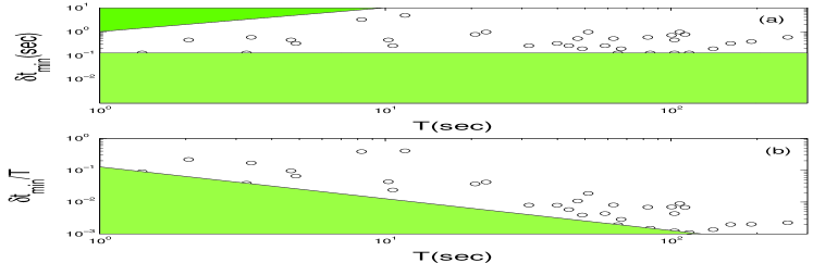
Figure 1: a) $\delta t_{min}$ and b) $\delta t_{min}/T$ as a function of the burst duration $T$ in long bursts. The gray areas are not allowed because of the resolution ($\delta t>128ms$) or the parameters definition $(\delta t\leq T)$

3.2 The effects of noise on the temporal structure

We turn now to the effect of noise on the time profile. We do so by comparing the attributes of the ’long’ sample with these of the ’noisy long’ sample (see 2.2). This procedure also tests our algorithm. Since we know the original signal (in the ’long’ sample) we can find out the efficiency of the algorithm in retrieving the attributes of the ’long’ sample out of the ’noisy long’ sample.

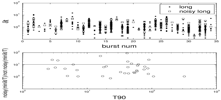
Figure 2: Top (a) : Pulses widths in the ’long’ (dots) and ’noisy long’ (squares) samples. Bottom (b) : The ratio between $\delta t_{min}/T$ in the ’long’ and ’noisy long’ as a function of BATSE’s $T_{90}$.

Fig. 2a represents all the pulses in the ’long’ and ’noisy long’ samples. The algorithm retrieves the basic features of the bursts out of the noisy sample. However, many pulses are ’lost’ because of the noise (only 30% of the ’long’ pulses are found in the ’noisy’ sample): (i) Some pulses are too weak to be distinguished within the amplified noise. (ii) Some pulses merge with others as the minimum between them are not statistically significant with the increased noise. The first effect does not affect the width of the pulses. However, the second one causes pulse widening. Therefore we expect fewer and wider pulses in the noisy sample. Both effects are seen clearly in Fig. 2. In the ’noisy’ sample there are 203 pulses with an average width of 1.62sec while in the original ’long’ sample there are 695 pulses with an average width of 1.39sec. The burst duration is affected by the noise as well, it becomes shorter. This happens when the first or the last pulses of the burst are lost.

These two effects (pulse widening and shorter burst duration) tend to increase the value of $\delta t_{min}/T$. Fig. 2b show that $\delta t_{min}/T$ increases by a factor of 10 in average, due to the noise. Thus the ratio $\delta t_{min}/T$ obtained from a noisy data can be considered as an upper limit to the real ratio.

3.3 Attributes of short bursts pulses

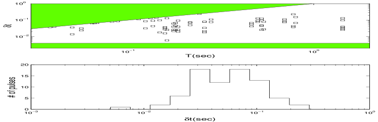
Figure 3: Top (a): The pulses widths in short bursts as a function of $T$. The gray areas are not allowed because of the resolution ($\delta t>4ms$) or the parameters definition $(\delta t\leq T$). Bottom (b): A histogram of the pulses widths in short bursts.

We have applied the same algorithm to the ‘short’ data sample. The pulses widths are shown as a function of the bursts duration in Fig 3 . The gray areas are not allowed because of the resolution ($\delta t>4ms$) or simply by ($\delta t\leq T$). Fig 3b depicts the distribution of the pulses width, $\delta t$. One can see that typical values of $\delta t$ are 50-100 ms with no significant correlation with T (provided we delete the smooth single peaked bursts with $\delta t\approx T$).

The pulse width found in this analysis is influenced by several effects. Some of this effects are due to our algorithm: First, few relatively close pulses could be seen by the algorithm as a single wide pulse. Second, the width of two pulses that are not well separated is determined by the minimum between the pulses. In this case the measured width of both pulses is shorter then their actual width.

There are also observational effects that influence the pulse width: First, as indicated in section 3.2, the pulses become wider by a factor of few because of the noise. Second, the resolution is limited. It is likely that the shortest pulses in the ’short’ sample are shorter then the best resolution of our data. Time scales shorter then the data resolution were already found in short bursts (Scargle, Norris & Bonnel 1997).

All the effects described above except one cause pulse widening. The exception is when two pulses overlap leading to a shortening of the estimated widths of both pulses. However, this effect rarely happens in our short bursts analysis. The S/N in this sample is very low, and the significance level we demand (4$\sigma$) is almost at the signal height (see sec. 2.1). Hence, a pulse determined by the algorithm is almost always well separated (otherwise the minimum between the pulse and its neighbor would be insignificant). Specifically 61 pulses out of the 65 pulses found in our sample are well separated: the minimum between pulses, on both sides, is lower than half of the maximum of the pulse. Thus, pulse widths are almost never underestimated. The combination of the other effects causes pulse widening. Hence our estimate of $\delta t_{min}/T$ , is only an upper limit.

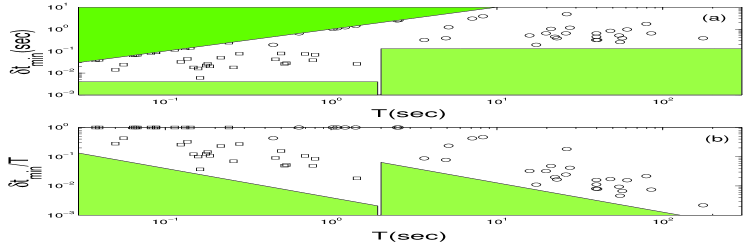
Figure 4: a) $\delta t_{min}$ and b) $\delta t_{min}/T$ as a function of the total duration of the burst for the ’short’ and the ’noisy long’ samples. The shaded areas are excluded because of the data resolution (4ms for shorts and 128ms for noisy longs) or the parameter definition ($\delta t_{min}<\leq T$).

Fig. 4 shows $\delta t_{min}$ and $\delta t_{min}/T$ for both groups ’short’ and ’noisy long’. In the ’short’ sample the median $\delta t_{min}/T$ is 0.25 while 35% of bursts have $\delta t_{min}/T\leq 0.1$ and 35% of the bursts show a smooth structure ($\delta t_{min}/T=1$). This result could mislead us to the conclusion that a significant fraction of the short bursts have a smooth time profile. But a look at the ’noisy long’ results show that also in this group more than 20% of the bursts are single pulsed, while there were no such bursts in the original ’long’ sample. Naturally, the bursts that loose the fine structure because of the noise are bursts with fewer original pulses. It is clear that short bursts have less pulses then long ones and therefore they are more “vulnerable” to this effect. Hence we conclude that at least one third of short bursts are highly variable ($\delta t_{min}/T\ll 1$) and it is very likely that another third (those bursts with $0.1<\delta t_{min}/T<1$)is variable as well. We cannot tell whether the smooth structure ($\delta t_{min}/T=1$) seen in a third of the short bursts is intrinsic or whether it arises due to the noise.

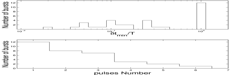
Figure 5: Top: The histogram of $\delta t_{min}/T$ in short bursts. Bottom: The histogram of the pulses number within a burst in the ‘short’ sample.

While we are mostly interested in this analysis in the pulse width, it is worth mentioning that the amplitude of the variations is large. In most (61 out of 65) cases, when there is no overlap of nearby pulses the number of counts drops to less than half of the maximal counts. Thus the pulse we describe are not only statistically significant, they also correspond to a significant (factor of 2) variation in the output of the source.

3.4 High resolution analysis of long bursts

We compare the time profile of the first seconds of 15 long bursts with the time profiles of 15 short bursts. Fig. 6 shows the light curves of a short burst and the first second of a long burst. The time scales of both bursts are quite similar. It is difficult to decide, on the base of these light curves alone, which one belongs to a short burst and which one is a fraction of a long one.

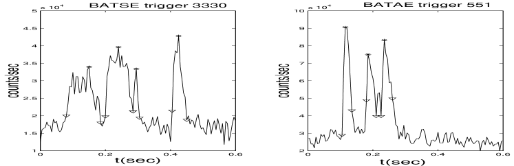
Figure 6: Left) The beginning of BATSE trigger 3330 (a long bright burst with $T_{90}=62sec$ ). Right) The whole light curve of BATSE trigger 551 (a bright short burst with $T_{90}=0.25sec$). The peaks found by our algorithm marked by stars. The triangles mark the pulses width. The figure demonstrates the similarity of short time scale structure in these bursts (at a 5 msec resolution).

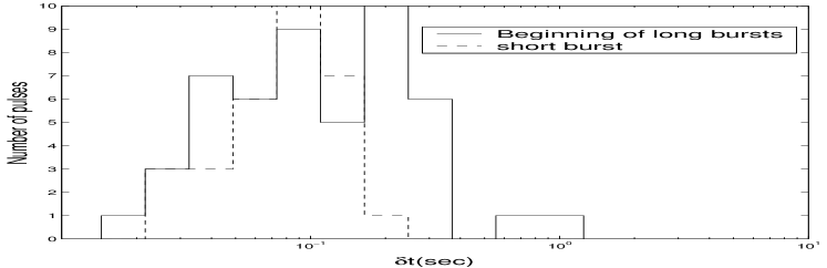
Figure 7: The histograms of pulses widths in the initial 1-2 seconds of long bursts (Smooth line) and pulses widths in short bursts (Dashed line). Both samples have a 5msec time bins.

Fig. 7 shows the pulse widths histograms of the beginning of long bursts and of the short bursts. The time scales in both samples are quite similar in the range of 10-200ms. The long bursts have additional pulses in the range of 0.2-1sec. Long bursts contain, of course, longer pulses, but in the sample we considered we demanded that the counts would fall back to the background level within the TTE data. In this way we have limited the pulses width of the long bursts. Both histograms begin at 10-20ms, which is at the limit of the pulse width resolution (10ms). It is likely that both samples contain shorter time scales that cannot be resolved.

The counts variations within the pulses observed in the high resolution long bursts is high. In 41 out of 46 pulses, the photon counts drops to less than half of the maximal counts of the pulse on both sides. Therefore, like in short bursts, the statistically significant variations in the bursts reflects also a significant variation in the output of the source.

Walker, Schaefer & Fenimore (2000) performed a similar analysis of TTE data of 14 long bursts. They found only one long burst with very short time scales. The difference between the results arises from the different samples considered. Walker et al. (2000) considered the bursts with maximal total photon counts within the TTE burst record. We demanded that the counts will return close to the background level within the TTE record. Walker et al. (2000) criterion favors bursts that are active during the whole TTE record and therefore most of the bursts in their sample are dominated by a long and bright pulse.

This similarity between the short bursts and the fraction of long bursts raises the question whether it is possible that short bursts are actually only a small fraction, which is above the background noise, of long bursts. We have already seen that the noise cause us to loose pulses. Is it possible that a long burst with a single dominant, very intense pulse, (or a group of very close and intense pulses) will loose all its structure, apart for this intense pulse, due to noise and become a short burst. Fig. 8 rules out this option. It depicts the counts ratio between the most intense pulse and the second most intense pulse within long bursts. The graph shows that in 32 out of 34 bursts the second highest peak is more then third of the most intense peak and in 27 bursts the second peak is more than two thirds of the first. The noise cannot cause one pulse to disappear without the other. As these two peaks are usually separated by more than two seconds, the noise cannot convert a significant fraction of long bursts to short ones. Clearly the noise has some effect on the duration histogram and in a few cases the added noise converted long bursts into a short ones, but it certainly cannot produce the observed bimodality.

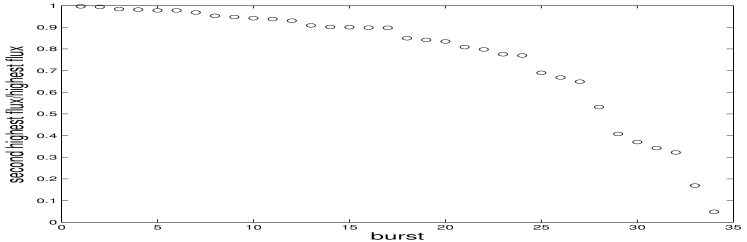
Figure 8: The ratio of the fluxes of the second brightest and the brightest peaks in long bursts.

4 Discussion

We have shown that most short bursts as well as most long bursts are multi-peaked and highly variable with $\delta t_{min}/T\ll 1$. These statistically significant variations involve generally a change of more than a factor of two in the count rate. 30% of the short bursts have a single pulse for which $\delta t_{min}$ is the same as the observed duration - $\delta t_{min}\approx T$. These are smooth bursts. However, a comparison with the ’noisy long’ sample, shows that this might be an artifact of the low S/N in the short bursts sample. We also find significant variability on very short time scale in long GRBs. This reduces the values of the variability parameter $\delta t_{min}/T$ to $10^{-3}-10^{-4}$ in long bursts.

External shocks (at least simple models of external shocks) cannot produce variable bursts (Sari & Piran, 1997; Fenimore, Madras & Nayakshin, 1996). Our result suggests that most short bursts are produced via internal shocks. 30% of the short bursts are smooth. We cannot rule out the possibility that these bursts are produced by external shock. The observed very short time scales in long GRBs strengthen further the argument in favor of internal shocks in these bursts and requires more contrived and fine tuned external shocks models for variability.

Kobayashi, Piran & Sari (1997) have shown that internal shocks cannot convert all the relativistic kinetic energy to gamma-rays. The remaining kinetic energy is dissipated latter when the relativistic ejecta is slowed down by the surrounding medium. The resulting external shocks produce the afterglow. An essential feature of this internal-external shocks scenario is that the afterglow is not a direct extrapolation of the initial $\gamma$-ray emission. This model suggests (Sari, 1997) for long bursts an overlap between the GRB and initial phase of afterglow. This have been indeed observed in several cases as a build up of a softer component during the GRB and a corresponding transition in the spectrum of long GRBs to a soft x-ray dominated stage towards the end of the burst.

For short GRBs the internal-external scenario suggests that the afterglow will begin few dozen seconds after the end of a short burst that was produced by internal shocks (Sari, 1997). It also suggest that this afterglow will not be a direct extrapolation of the GRB (as the two are produced by different mechanisms). Thus we predict that for most short bursts there will be a gap between the burst and the beginning of the afterglow. We have already remarked that at this stage one cannot tell whether the remaining 30% smooth short bursts are produced by external or by internal shocks. This could be tested in the distant future with better data. However, there are clear predictions concerning the afterglow that could distinguish between the two possibilities. If these short GRBs are produced by internal shocks then we expect a clear gap between the end of the GRB and the onset of the x-ray afterglow. If on the other hand these short bursts are produced by external shocks then we predict that the afterglow would continue immediately with no interpretation after the GRB and its features would be a direct extrapolation of the properties of the GRB.

Appendix -The algorithm

Our algorithm finds the peaks of the bursts. Each peak corresponds to a single pulse; a pulse is the basic event of the light curve. The algorithm is based on the algorithm suggested by Li & Fenimore (1996). Li & Fenimore define a time bin $t_{p}$ (with count $C_{p}$) as a peak if there are two time bins $t_{1}<t_{p}<t_{2}$ (with counts $C_{1},C_{2}$ respectively) which satisfies a) $C_{p}-C_{1,2}>N_{var}\sqrt{C_{p}}$ and b) $C_{p}$ is the maximal count between $t_{1}$ and $t_{2}$. $N_{var}$ is a parameter that determines the significance of the peak.

There are two problems with this algorithm. First, this algorithm analyzes only data in a single time resolution (fixed time bin size). Therefore the algorithm looses long and faint pulses. A peak that does not satisfy the criterion described above in the raw data resolution could satisfy the criterion if the data resolution is lower (longer time-bins). This algorithm would miss such a pulse. Second, $N_{var}$ determines the trade-off between sensitivity and false peaks identification rate. When $N_{var}$ is low the algorithm finds false peaks as a result of the Poisson noise. When $N_{var}$ is high the algorithm misses real peaks. Finding false peaks is a severe problem during long periods of constant level Poisson noise, like the background (as will be explained shortly). Long bursts contain such periods (periods of only background noise). These periods are called quiescent times. In order to avoid false peaks in long bursts $\textrm{N}_{\textrm{var }}$must be large($\geq 7$), which means an insensitive algorithm. Short bursts contain less quiescent times, and of course shorter ones. But, short bursts contain much less pulses then long burst (three to four compared to an average of more than thirty) and much smaller S/N. Finding even one false peak could change the features of the burst drastically. Too insensitive algorithm could loose all the burst structure. In order to avoid false peaks in short bursts $\textrm{N}_{\textrm{var }}$must be at least as large as 5. As described in section 2.1, the S/N in some of the bright short bursts is smaller than 5. Such $N_{var}$ will prevent the algorithm from finding even one peak in these bursts.

We solved the first problem by analyzing the data in different resolutions. The results of the algorithm in different resolutions are merged into a single sample of peaks. We solved the second problem by restricting the search for peaks only to ‘Active Periods’. Active periods are periods with counts that correspond to source activity (we will define it later on).

There are few advantages for analyzing only active periods. The main one is that a lower $N_{var}$ can be used during these periods with smaller risk of finding false peaks. The risk of finding false peaks due to a Poisson noise depends on the time scale in which the original signal (i.e. without the noise) changes its count rate in the same order as the Poisson noise level. If the signal is constant (no real pulses), then this time scale is as long as the signal. If the constant signal is longer, it contains more time bins with the same level of Poisson noise counts. Hence, there is a larger chance of finding within these time-bins three time-bins, $t_{p}$, $t_{1}$ and $t_{2}$, that satisfy the criterion in Li & Fenimore algorithm. Then $t_{p}$ would become a false peak. On the other hand, if the signal is changing monotonically then the length of the signal is irrelevant. $t_{p}$, $t_{1}$ and $t_{2}$ must be within the period in which the signal changes at the same order as the Poisson noise level; there is no chance of finding $t_{2}$ with $C_{2}$ significantly below $C_{p}$ (if the signal is rising) out of this period. During the active periods the signal is changing rapidly (usually on time scales of seconds or less), and the Poisson noise is superimposed on steep slopes. In this case a false peak could only be found during the period in which the signal didn’t change compared to the noise level. There are much less time bins during this period and hence there are much less chance of finding false peaks.

The second advantage is that when an active period is found we almost certain that it is a part of the burst. This is important since one false peak in the ‘wrong’ place (for example hundred of seconds after the burst ended) can change the burst properties drastically. By analyzing only active periods we can use smaller $N_{var}$ (=4) and get a more sensitive and accurate algorithm.

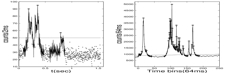
Figure 9: Left) Time profile of BATSE trigger 2952 (bright short burst). Right) Time profile of BATSE trigger 2156 (bright long burst). The solid line marks the active periods. The horizontal line marks the activity level. All the time bins with counts above the activity level are ‘active bins’. The peaks are marked by ’*’.

Our algorithm works in several steps. First, it determines the background level of the signal (as a function of time). Then it finds an activity level, demanding a probability of 0.9 (per burst) that all the time bins with counts above this level (called ‘active bins’) correspond to source activity and not of the background Poisson noise (we demand that on every ten bursts there is, on average, a single false ‘active bin’). The activity level depends on the background and its value is between 4$\sigma$ to 5$\sigma$ above the background. From each active bin we search to the right and to the left until the count level drops to the background level on both sides. We call all these bins together an active period (from the time bin that the counts are above the background until the time bin that the counts reaches the background level again). In most cases a single active period includes many active bins and a burst may contain more then a single active period (see Fig 9). Note that if the algorithm misses an active period in one resolution, it can still find it in a different (lower) resolution, in which the noise level is lower.

Once the active periods of a given burst have been determined we apply the Li & Fenimore algorithm to the active periods (using Nvar=4) and determine the peaks. We repeat this procedure (finding the active periods and the corresponding peaks), several times for different time resolution. To obtain lower resolution data we convolve the original signal (in the basic time bins) with a Gaussian, whose width determines the resolution. Finally, after finding the peaks in different resolutions we merge those samples of peaks to a single sample (requiring that a peak must appear in at least two different resolutions). The merge is done by merging the highest resolution sample with the second highest one and then taking this merged sample and merging it with the third highest resolution sample and so on. On different resolutions the same peak could be found on different time bins. In each case two peaks on different resolutions are considered as a single one if the peak in one resolution falls between $t_{1}$ and $t_{2}$ of the peak in the other resolution.

Each peak corresponds, of course, to a pulse. The pulse width ($\delta t$) is defined by two points (on each side of the peak) that are higher than the background by 1/4 of the peaks height or by the minimum between two neighboring peaks (if the latter is higher). The duration ($T$) of the burst is the time elapsed from the beginning of the first pulse till the end of the last pulse (so in single pulsed burst $T=\delta t$).

References

- [1] Beloborodov A. M., Stern B. E., Svensson R., 2000, ApJ, 535, 158
- [2] Cline D. B., Matthey C., Otwinowski S., 1999, ApJ, 527, 827
- [3] Kobayashi S., Piran T. Sari R., 1997, ApJ, 490, 92
- [4] Lee A., Bloom E., Scargle J., 1995, in Kouveliotou C., Briggs M. S., Fishman G.J., Eds., AIP Conf. Proc. 3rd Huntsville Symposium, Gamma-Ray Bursts, p.47 (New York: AIP)
- [5] Lee A., Bloom E. D., Petrosian V., 2000, ApJS, 131, 21
- [6] Li H., Fenimore E. E., 1996, ApJ, 469, L115
- [7] Fenimore E. E., Madras C. D., Nayakshin S., 1996, ApJ, 473, 998
- [8] Norris J. P., Nemiroff R. J., Bonnell J. T., Scargle J. D., Kouveliotou C., Paciesas W. S., Meegan C. A., Fishman G. J., 1996, ApJ, 459, 393
- [9] Norris J. P., 1995, in Kouveliotou C., Briggs M. S., Fishman G.J., Eds., AIP Conf. Proc. 3rd Huntsville Symposium, Gamma-Ray Bursts, p.13 (New York: AIP)
- [10] Sari R.,1997, ApJ, 489, L37
- [11] Sari R., Piran T., 1997, ApJ, 485, 270
- [12] Scargle J. D., 1998, ApJ, 504, 405
- [13] Scargle J. D., Norris J., Bonnel J., 1997 in Meegan C., Preece R., Koshut T., Eds., AIP Conf. Proc. 4th Huntsville Symposium, Gamma-Ray Bursts, p.181 (New York: AIP)
- [14] Walker K. C., Schaefer B. E. , Fenimore, E. E., 2000, ApJ, 537, 264