Empirical relations for cluster RR Lyrae stars revisited

Our former study on the empirical relations between the Fourier parameters of the light curves of the fundamental mode RR Lyrae stars and their basic stellar parameters has been extended to considerably larger data sets. The most significant contribution to the absolute magnitude $M_{V}$ comes from the period $P$ and from the first Fourier amplitude $A_{1}$, but there are statistically significant contributions also from additional higher order components, most importantly from $A_{3}$ and in a lesser degree from the Fourier phase $\varphi_{51}$. When different colors are combined in reddening-free quantities, we obtain basically period$-$luminosity$-$color relations. Due to the $\log T_{\rm eff}(B-V,\log g,{\rm[Fe/H]})$ relation from stellar atmosphere models, we would expect some dependence also on $\varphi_{31}$. Unfortunately, the data are still not extensive and accurate enough to decipher clearly the small effect of this Fourier phase. However, with the aid of more accurate multicolor data on field variables, we show that this Fourier phase should be present either in $V-I$ or in $B-V$ or in both. From the standard deviations of the various regressions, an upper limit can be obtained on the overall inhomogeneity of the reddening in the individual clusters. This yields $\sigma_{E(B-V)}$_∼^<0.012 mag, which also implies an average minimum observational error of $\sigma_{V}$_∼^>0.018 mag.

1 Introduction

In recent years we have conducted a series of studies aimed at deriving empirical relations between the Fourier parameters of the light curves and the physical parameters of the RR Lyrae stars (Jurcsik & Kovács 1996; Kovács & Jurcsik 1996, 1997; hereafter JK96, KJ96, KJ97, respectively). The method is purely empirical, and based on the assumption that the period and the shape of the light curve are directly correlated with the physical parameters (or quantities related to them), such as the absolute magnitude $M_{V}$, intrinsic color $(B-V)_{0}$ and metal abundance [Fe/H]. Therefore, it is hoped that once the formulae are derived for a representative sample, the relative values of the above physical parameters can be determined for any other RR Lyrae star, assuming that accurate light curve parameters in $V$ color are available.

The advantage of this method would be the utilization of very accurate observables (period, Fourier parameters) in calculating individual stellar parameters. If it were possible to fit a large number of calibrating objects (in the present study, globular cluster variables) with the accuracy of the observational noise, this would imply a precise calculation of the relative physical parameters from the derived formulae. In addition to the more practical applications of relative distance and reddening determinations, the ultimate goal is to reach the level of accuracy at which a direct (star by star) comparison with the evolutionary calculations becomes possible.

In JK96 we used Galactic field RR Lyrae stars for the derivation of the [Fe/H] formula. The expression was shown to give reliable abundances also for cluster stars, except perhaps at the low abundance end, where our formulae predict somewhat higher abundances. (However, we note that this result is based on the average cluster values obtained from direct abundance analyses of giants and not of RR Lyrae stars. Recent spectroscopic investigations of Behr et al. (1999) indicate that substantial abundance differences might exist even within the horizontal branch.)

The relations for $M_{V}$ and $(B-V)_{0}$ were obtained from globular cluster stars (see KJ96 and KJ97). If we assume that cluster and field RR Lyrae stars cover overlapping evolutionary stages and physical parameter space, then these latter formulae can also be applied to the field stars. The validity of this statement depends crucially on the completeness of the calibrating sample. Recent ccd photometric studies of cluster RR Lyrae stars allow us to satisfy this condition more closely in the present investigation than in our former studies, and revisit the problem of absolute magnitude and color calibrations. Both the quality and the quantity of these new data lead to better determination of the number of significant Fourier parameters entering in the formulae and, at the same time, to a more accurate calculation of the regression coefficients.

2 The new empirical formulae

The clusters and the corresponding number of variables together with the sources of the data are summarized in Table 1. This table contains all fundamental mode RR Lyrae (RRab) stars from the given sources, except those with: (a) obvious amplitude modulation (Blazhko effect), (b) clear outlier status due to e.g., cluster non-membership, (c) poor quality light curves, (d) short periods and sinusoidal light curves (e.g., V73, 76, 169, 185, 189 in $\omega$ Cen and V70 in M3). Fourier parameters of the $V$ light curves and average colors used in this paper are given in Table 2.

Table 1: Summary of the globular cluster data for RRab stars

Cluster	$N_{B}$	$N_{V}$	$N_{I}$	Source
M2	13	13	–	LC99
M3	–	28	–	K98
M4	4	5	3	KJ97
M5	12	43	24	K00, KJ97
M9	–	4	–	CS99
M55	4	4	–	O99
M68	5	5	5	W94
M92	5	4	3	KJ97
M107	–	7	–	CS97
NGC1851	11	11	11	W98
NGC5466	7	7	–	C99
NGC6362	12	12	10	W
NGC6981	20	20	18	W
IC4499	49	49	41	WN96
Rup. 106	12	12	–	K95a
$\omega$ Cen	–	44	–	K97
Sculptor	–	90	–	K95b
NGC 1466	8	8	–	W92b
NGC 1841	9	9	–	W90
Reticulum	8	8	–	W92a
Total :	179	383	115

References: CS97: Clement & Shelton (1997); CS99: Clement & Shelton (1999); C99: Corwin et al. (1999); K95a: Kaluzny et al. (1995a); K95b: Kaluzny et al. (1995b); K97: Kaluzny et al. (1997); K98: Kaluzny et al. (1998); K00: Kaluzny et al. (2000); KJ97: Kovács & Jurcsik (1997); LC99: Lee & Carney (1999); O99: Olech et al. (1999); W90: Walker (1990); W92a: Walker (1992a); W92b: Walker (1992b); W94: Walker (1994); WN96: Walker & Nemec (1996); W98: Walker (1998); W: Walker (unpublished);

Color indices and average $V$ colors are calculated from the same source, except for M5. In the case of this cluster we average the $V$ values used by KJ97 and the ones published by Kaluzny et al. (2000) for all common stars in the two publications. In comparison with KJ96 and KJ97, we see that there is more than a factor of two increase in the number of stars in all colors (this is so even though in the present data sets we have omitted all photographic and less accurate ccd data used in our previous analyses). The large sample enables us to deal with separate data sets and obtain further information on the statistical significance of the various regressions.

For deriving the relations between the Fourier parameters, absolute magnitudes and colors, we follow the same methodology as in our former studies. For example, in the case of $M_{V}$, the best regression is obtained from the minimization of the following expression

$${\cal D}^{2}={1\over N^{\ast}}\sum_{j=1}^{N_{c}}\sum_{i=1}^{N_{j}}\Bigl{[}V_{j}(i)-\tilde{d}_{j}-m_{0}-\sum_{k=1}^{N_{p}}m_{k}{\cal F}_{k}(i)\Bigr{]}^{2}\hskip 5.69054pt,$$ (1)

where $N^{\ast}=N-N_{c}-N_{p}$, $N$ is the total number of stars, $N_{c}$ is the number of clusters, $N_{p}$ is the number of the Fourier parameters, $N_{j}$ is the number of stars in the $j$-th cluster, $V_{j}(i)$ is the observed average magnitude of the $i$-th star in the $j$-th cluster. The Fourier parameters (including the period) are denoted by ${\cal F}_{k}(i)$. The least-squares minimization leads to the determination of the relative reddened distance moduli $\tilde{d}_{j}$ and the regression coefficients $m_{k}$. The zero point of the magnitude scale $m_{0}$ is absorbed in the distance moduli and should be determined from some direct distance calibration (e.g., parallaxes, Baade-Wesselink analyses, double-mode variables, etc., however, please note that the absolute magnitude scale of the RR Lyrae stars is still an unsettled issue — e.g., Stanek et al. 2000 vs. Feast 1999 and Kovács 2000).

For each fixed $N_{p}$ we check all possible combinations from the period $P$ and from the first five Fourier amplitudes and phases ($A_{1}$, …, $A_{5}$; $\varphi_{21}$, …, $\varphi_{51}$ — see Simon & Teays (1982) and JK96 for the definition of these quantities). After finding the best fit, we repeat the procedure with another $N_{p}$ ($\leq 8$). The optimum fit is obtained at the lowest parameter number for which the fitting accuracy ${\cal D}$ starts to become constant. Throughout this paper we use linear combinations of the Fourier parameters. We have not found any clear sign of preference for using nonlinear combinations either for the fitting or for the fitted quantities.

Three observables, related to static (or more accurately, to pulsation-cycle-averaged) stellar parameters, are studied. The first one is the intensity averaged $V$ magnitude. The advantage of this quantity is that it is directly related to the absolute magnitude $M_{V}$ of the static star (cf. Bono, Caputo & Stellingwerf 1995). The disadvantage of the $V$ magnitude is that it is strongly affected by inhomogeneous cluster reddening which may be important in some clusters. From this point of view, a better approach is fitting reddening-free quantities, such as $W=V-R_{V}(B-V)$ and $X=V-R_{I}(V-I)$, where $R_{V}$ and $R_{I}$ are the extinction ratios (e.g., Cardelli, Clayton & Mathis 1989; Liu & Janes 1990). Here we set $R_{V}=3.1$, $R_{I}=2.5$ (the latter value corresponds to the Kron-Cousins system in $I$ color). We use magnitude averages both in $W$ and in $X$, because there does not seem to be a strong preference toward other averages when a comparison is made between the static and average color indices in the nonlinear pulsation models (Bono et al. 1995). The observed and intrinsic quantities are related through the true distance modulus

$$W=W_{0}+d\hskip 5.69054pt,$$ (2)

and similar expression holds also for $X$. Our task is to derive relations between the Fourier parameters and the intrinsic quantities. For the calculation of the distance modulus in the case of other values of $R_{V}$ and $R_{I}$ than the ones used in this paper, the expressions derived here for $W_{0}$ and $X_{0}$ can still be used but the distance modulus should be modified according to KJ97.

The price we have to pay for eliminating reddening in $W$ and $X$ is the amplification of the observational noise due to the large values of $R_{V}$ and $R_{I}$. If the reddening is sufficiently small, it is obvious that using $W$ and $X$ is not the best idea, because of the unnecessarily amplified observational noise. Therefore, for any noise in the reddening and in the $B$ and $V$ magnitudes, there is an optimum trade-off between filtering out reddening fluctuations and keeping the effect of observational noise at minimum. Indeed, the expression for the variance of $W=V-\alpha(B-V)$ shows this property

$$\sigma^{2}_{W} = (R_{V}-\alpha)^{2}\sigma^{2}_{E}+\alpha^{2}\sigma^{2}_{B}+(1+\alpha)^{2}\sigma^{2}_{V}-$$ (3)

$$- 2\alpha(1+\alpha)K\sigma_{V}\sigma_{B}\hskip 5.69054pt.$$

Here $\sigma_{E}$, $\sigma_{B}$ and $\sigma_{V}$ are the standard deviations of the reddening, $B$ and $V$ magnitudes, respectively, and $K$ is the correlation coefficient of $V$ and $B$. Although tests with the observed data and the study of the above equation indicate that $\alpha\approx 1.5$ – $2.0$ would be more preferable than $\alpha=R_{V}$, the gain is only about 10% in the increase of the fitting accuracy. This improvement does not seem to justify the giving up of the more transparent approach based on standard extinction ratios.

A general problem in searching for the best-fitting linear combination in the form of Eq. (1) is that the Fourier parameters ${\cal F}_{k}(i)$ are not independent. For the period and the total amplitude this correlation has been known for a long time (Preston 1959). As is shown in Fig. 1, there are approximate correlations also with the other Fourier parameters. Note that the scatter in these diagrams has a physical origin, because the accuracy of the low-order Fourier parameters is very high (better than $1\%$ if only the observational errors are considered, but may be less accurate than this in the case of hidden Blazhko variables — see also Sect. 2.1 for the discussion of the total errors in the Fourier parameters). One of the reasons for the scatter in Fig. 1 is that there are metallicity differences between the clusters. Assuming constant [Fe/H] for a given cluster, we would expect straight lines shifted vertically in the $P\rightarrow\varphi_{31}$ diagram (see JK96). Because of the relatively narrow range, overlapping distributions of [Fe/H] in different clusters and chemical inhomogeneity in several clusters, this ridge structure is not seen in the figure. Other phases show similar progression, due to their tight interrelations with $\varphi_{31}$ (JK96, see Kovács & Kanbur 1998 for an update of these relations). The scatter in the amplitudes is only partially due to metallicity effects (they yield much weaker correlation with [Fe/H] than the phases — see JK96). Because of the significant amplitude dependence of the luminosity and temperature, the rest of the scatter is attributed to the variation of these quantities.

The problem of the internal correlation of the Fourier parameters can be circumvented by constructing an orthogonal set with the aid of principal component analysis (see Kanbur, Mariani & Iono 2000). Although this approach certainly results in a better posed numerical scheme, both methods should end up with the same conclusion, because both of them use linear combinations of the same set of Fourier parameters. More sophisticated methods, such as the one mentioned, could be instrumental in the future studies of the finer (high frequency) details of the light curves, when the Fourier decomposition becomes a non-useful concept.

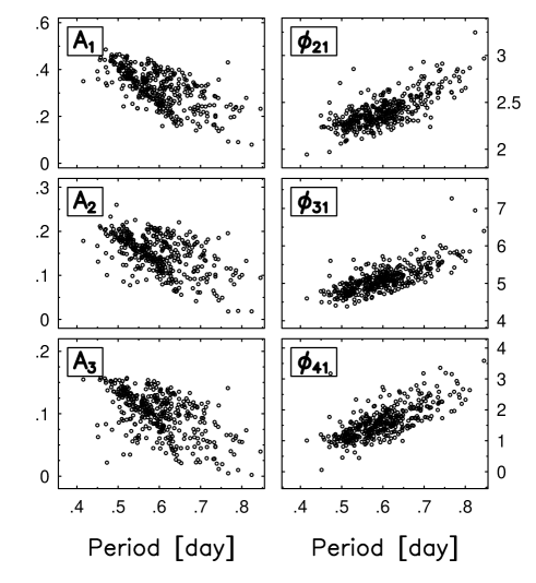
Figure 1: Fourier parameters of cluster RRab stars

2.1 The absolute magnitude $M_{V}$

Because we have a large number of stars observed in $V$ color, we are in the position to test the significance of the derived formulae on two independent data sets. In Table 3 we show the distribution of the clusters in the two sets. The clusters are sorted in the two groups by following the guideline of yielding about the same number of stars and including good quality large samples in both sets.

Table 3: Data sets for the $M_{V}$ fit

$A$	$B$	$C$
$N_{\phantom{c}}=191$	$N_{\phantom{c}}=192$	$N_{\phantom{c}}=383$
$N_{c}=15$	$N_{c}=5$	$N_{c}=20$
M2, M3, M4, M9,	M5, $\omega$ Cen,	A & B
M55, M68, M92, M107,	N5466, Sculptor,
Rup 106, N1851,	Reticulum
N6362, N6981, IC4499,
N1466, N1841

In searching for the best fitting formula, we successively leave out those stars which can be regarded as outliers. This could be a somewhat delicate procedure, especially in the case of small sample size or noisy data, such as the samples used in our former investigations. In this work we are more conservative than in our previous studies and confine ourselves to secure outliers which exceed the $\approx 3\sigma$ limit. The list of these stars is given in Table 4. We see that there are 17 variables which do not conform to the relation required by the rest of the sample. This means a $4\%$ chance that the derived formula yields incorrect results in a randomly chosen sample of RRab stars (assuming that the sample does not contain ‘obvious’ Blazhko variables or stars with blended components). The chance of error may be even smaller, because some of the discarded stars might be Blazhko variables which would have been omitted if we had longer photometry available. Some of the stars listed in Table 4 show reasonably clear signs of observational or other defects. For example, V20 in N1851 and V16 in M2 have excessive scatter in their light curves. Blending or unresolved close components might be suspected in V118 of $\omega$ Cen and in V01446 and V02575 of Sculptor. Additional, more detailed examination of these and other stars are needed to clarify the reasons for their outlier status.

Table 4: Outliers in the various regressions

Regression	Outliers
$M_{V}$ …..	M2: V4, 16, M5: V27, 59, M107: V10,
	$\omega$ Cen: V109, 118, 150, 154, N1851: V20,
	Sculptor: V01446, 02575, 06032, 06034,
	IC4499: V76, N1466: We14, N1841: V19
$W_{0}$ …..	M2: V16, M5: V59, 86, M92: V4,
	N1851: V20, IC4499: V167, Rup. 106: V10
$X_{0}$ …..	M5: V13, 27, 59, 83, N1851: V20,
	IC4499: V34

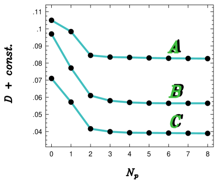
Figure 2: Standard deviation of the residuals of the $M_{V}$ fit as a function of the number of the regression parameters. Results displayed for data sets $A$ and $B$ are vertically shifted for better visibility ($const.=0.048$, $0.015$ and $0.0$ for sets $A$, $B$ and $C$, respectively

Fig. 2 shows the significance of the derived formulae. The standard deviations at $N_{p}=0$ are equal to the averages of the standard deviations of the observed magnitudes in each cluster. We see that the decrease of the unbiased estimates of the standard deviations for parameter numbers greater than 2, is very small. Therefore, the present data seem to suggest the existence of a relation which contains only 2 parameters. This is in conflict with our previous result, where we argued for the validity of a 3 parameter formula. Before we draw a conclusion, it is necessary to test if the smaller change of ${\cal D}$ in the case of the high parameter fits is statistically significant. Because of the complexity of the fitting procedure (e.g., the use of noisy Fourier parameters), it is not possible to apply standard methods of analysis of variances (e.g., Sachs 1982). Instead, direct numerical tests are performed. More specifically, in testing data set $C$, the procedure below is followed.

For each parameter number $N_{p}$, synthetic data are generated by using the formula obtained from the given data set. Then, Gaussian noise is added both to these data and to all Fourier parameters i.e., the test data have the following form:

$$v_{j}(i)=\tilde{d}_{j}+\xi_{j}(i)+\sum_{k=1}^{N_{p}}m_{k}[{\cal F}_{k}(i)+\eta_{k}(i)]\hskip 5.69054pt.$$ (4)

In these tests the role of the exact values of the relative distance moduli $\tilde{d}_{j}$ is not essential. Therefore, we take simply the average $V$ magnitudes in each cluster as very rough substitutes for the exact values. The noise components are chosen in such a way as to yield the observed standard deviation at the given $N_{p}$. Because the observed standard deviation is a result of the errors of the Fourier parameters and of the average magnitudes, $\sigma_{\xi}$ is slightly smaller than the observed standard deviation. Unfortunately, the accurate values of the errors of the Fourier parameters are not known. Although the formal statistical errors can be computed, because of the larger dispersion of the interrelations, there might be additional sources of errors (e.g., Blazhko effect, background contamination). From the updated relations of Kovács & Kanbur (1998) we think that the values of $\sigma(A_{i})=0.01$ and $\sigma(\varphi_{i1})=0.03$ are reasonable estimates for the overall total errors of the low-order Fourier parameters. These values are used at all $N_{p}$ in the following simulations. The adjusted standard deviations of $\xi_{i}$ are $0.057$, $0.041$, $0.039$, $0.038$ and $0.037$ for $N_{p}=1$, $2$, $3$, $4$ and $5$, respectively. We note that these standard deviations are up to $0.002$ smaller than the observed ones shown in Fig. 2.

For each realization of the data generated above, standard parameter searches are performed, similar to the observed data. By repeating the analysis for many realizations, information is obtained on the significance of the regression at parameter number $N_{p}$.

The following statistical parameters are calculated:

• $P_{i}$: probability of the identification of the parameter set used in the generation of the synthetic data.

• $\sigma_{par}^{max}$: maximum of the relative standard deviations of the regression coefficients ($\sigma_{par}^{max}=max\{\sigma(m_{k})/|m_{k}|\}$).

• $\Delta={\cal D}^{2}(N_{p})-{\cal D}^{2}(N_{p}+1)$ and its standard deviation $\sigma_{\Delta}$.

• $S=(\Delta_{obs}-\Delta_{test})/\sigma_{\Delta}$, the significance of the $N_{p}+1$ versus the $N_{p}$ parameter fits.

The results of the above test on data set $C$ are shown in Table 5.

Table 5: Statistical test of the significance of the various $M_{V}$ regressions on data set $C$ (see text for details)

$N_{p}$	$P_{i}(\%)$	$\sigma^{max}_{par}(\%)$	$\Delta_{obs}$	$\Delta_{test}$	$\sigma_{\Delta}$	$S$
1	$100$	$\phantom{2}7$	$1541$	$19$	$18$	$85$
2	$100$	$\phantom{2}6$	$\phantom{1}139$	$15$	$13$	$\phantom{8}9$
3	$\phantom{1}67$	$27$	$\phantom{15}47$	$11$	$\phantom{1}9$	$\phantom{8}4$
4	$\phantom{1}62$	$27$	$\phantom{154}8$	$10$	$\phantom{1}9$	$\phantom{8}0$
5	$\phantom{1}36$	$55$	$\phantom{154}8$	$\phantom{1}8$	$\phantom{1}8$	$\phantom{8}0$

Note: $\Delta_{obs}$, $\Delta_{test}$ and $\sigma_{\Delta}$ are in $10^{-6}$ mag²

We see that the two parameter regressions are undoubtedly very significant in all test quantities. Furthermore, a little closer examination of the three and four parameter regressions leads to the conclusion that these higher parameter formulae are also significant (although the four parameter one might be close to the detection limit). The present data render any further increase of the parameter number to be statistically insignificant. This result is basically in line with the conclusion of KJ96, although here we get $A_{3}$ and $\varphi_{51}$ for the higher parameters, whereas in KJ96 we obtained $\varphi_{31}$. This difference is attributed to the smaller data set used in KJ96 and to the interrelations between the Fourier parameters, already mentioned at the beginning of this section. We return to the compatibility of this work and that of KJ96 in Sect. 4.

In column 5 the $\Delta_{test}$ values are positive, although we would expect zero, since at any $N_{p}$ the higher parameter regressions fit only the noise, which should give zero $\Delta_{test}$ on the average, because this quantity is calculated from the unbiased estimates of the standard deviations (see Eq. (1)). The reason why we get small positive values is that in the $N_{p}+1$ parameter search, those parameter combinations are selected which yield the smallest dispersion from the ones which employ $N_{p}+1$ parameters from the first 10 Fourier components. Therefore, there is a better chance to get some decrease in the dispersion then if we had only one additional component to use in the $N_{p}+1$ parameter fit.

We note that if we did not use noise in the Fourier parameters, we would reach the same conclusion about the parameter number, although with an even higher significance.

Formulae obtained for $M_{V}$ with various parameter numbers from data sets $A$, $B$ and $C$ are given in Table 6.

Table 6: Formulae for $M_{V}$ obtained from various data sets

Set	$M_{V}+const=$	${\cal D}$
A	$-1.682\log P-0.736A_{1}$	0.0365
B	$-1.897\log P-0.855A_{1}$	0.0460
C	$-1.820\log P-0.805A_{1}$	0.0416
C	$-1.876\log P-1.158A_{1}+0.821A_{3}$	0.0399
C	$-1.963\log P-1.124A_{1}+0.830A_{3}$
	$\phantom{-1.963\log P-1.124A_{1}}+0.011\varphi_{51}$	0.0393

• • — phase $\varphi_{51}$ must be in the [3.5,5.5] interval

  • — outliers have been omitted according to Table 4

The $10\%$ difference between the coefficients of $\log P$ of the formulae derived on sets $A$ and $B$ can be accounted for by the errors in the coefficients (the $1\sigma$ relative errors of the regression coefficients are $\approx 4\%$ for both data sets). The two formulae yield also very similar $M_{V}$ values. A comparison made on a sample of $\approx 500$ stars compiled from Galactic field and cluster variables, gave $0.011$ mag for the standard deviation of the differences between the $M_{V}$ values computed from these formulae. Considering the total range of $M_{V}$ (which is $\approx 0.6$ mag for this large data set and $\approx 0.4$ mag for the clusters), this standard deviation corresponds to compatibility at the 2% level. For data set $C$ we see changes in the coefficients with the variation of the parameter number. This is primarily due to the interrelations among the Fourier parameters. As is expected, the differences between the various $M_{V}$ estimates obtained from the high- and low-parameter formulae are rather small. By using the above large data set, we get $\sigma=0.012$ and $0.008$, if we compare the two and three, and three and four parameter formulae, respectively. Since — as we have already seen — the three and possibly even the four parameter formulae are significant, this comparison gives some indication on the accuracy to be gained by the application of the high parameter formulae (however, this gain is partially counterbalanced by the statistical errors of $M_{V}$ — see Appendix A). This level of change in $M_{V}$ is not very important in simple applications (e.g., in distance modulus calculations), but could have interesting consequences when empirical evolutionary tracks are attempted to be calculated.

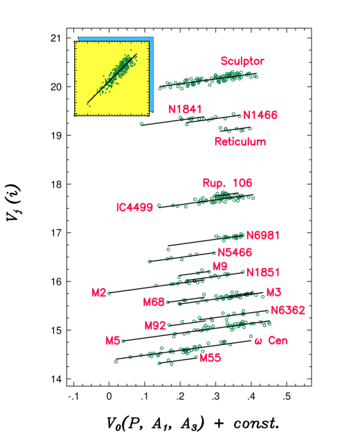
Figure 3: Observed $V$ magnitudes versus absolute magnitudes ($V_{0}$, calculated from Eq. (5)). Lines show fiducial values obtained from $V_{0}$ after shifts with optimum distance moduli. Inset displays the same quantities after adjustment of the $V$ magnitudes by the relative distance moduli

Fig. 3 displays the correlation between the observed and calculated magnitudes. (It is noted that M107 and M4 are not plotted. For M107 the reddened distance modulus is equal to that of M3. The cluster M4 is omitted, because plotting would result in a large crowding in the figure due to its high observed brightness.) The calculated magnitudes are obtained from the three parameter fit to the magnitude averaged values. This yields the following formula for data set $C$

$$V_{0}=-1.880\log P-0.971A_{1}+0.909A_{3}+const.\hskip 5.69054pt.$$ (5)

The slight difference between this and the corresponding formula in Table 6 is due to the different ways of averaging of the observed magnitudes. The above formula fits the data with $\sigma=0.040$ mag. The nice correlation with the variables of the individual clusters is very comforting. This shows that with a good chance, no important physical dependence in $V_{0}$ (or in $M_{V}$) are missed in the above derivation. The method could have been a failure if $M_{V}$ were a single function of [Fe/H] and, at the same time, the clusters were chemically homogeneous. This situation would lead to ‘truly horizontal branches’, which would mean the absorption of all physical parameters into the (incorrect) distance moduli and the lost of any correlation with the Fourier parameters. Both chemical inhomogeneities and complex parameter dependence of $M_{V}$ prevent this situation from happening. Since most of the clusters have reasonably small [Fe/H] dispersion, we can conclude that the empirical [Fe/H]—$M_{V}$ relation is rather loose, as has already been shown in KJ96.

2.2 The $PLC$ relation for $B$, $V$

We use the data sets given in Table 7 to find the optimum formula for the reddening-free quantity $W$. By following the same procedure as in the $M_{V}$ fit, outliers are omitted iteratively. The list of the 7 stars which were left out from the final samples is given in Table 4. On the basis of the small number of outliers we find similar ‘applicability ratio’ of the derived formulae as in the case of the $M_{V}$ fit. The variation of the fitting accuracy as a function of the parameter number is shown in Fig. 4. The single parameter nature of $W$ seems to be very strongly indicated. This result is at variance with the conclusion of KJ97, who argued for the significance of a 3 parameter relation. The reason of this contradiction is that KJ97 used considerably smaller sample with larger observational noise (e.g., photographic data for N3201 and M107). This resulted in a somewhat biased selection of the outliers, and a concomitant overestimation of the parameter number. Nevertheless, as we shall see in Sect. 4, the derived formulae give similar results.

Table 8 shows that data sets $a$ and $b$ yield almost the same single parameter formulae. In the last row we also display the two parameter formula which might be suspected as the highest parameter relation allowed by the present data set for $W_{0}$. Although the absolute change in $\cal D$ is similar to the one observed between the three and four parameter formulae for $M_{V}$, here the statistical significance is even lower, because of the more than a factor of two lower number of data. Indeed, repeating the same type of numerical test as in the case of $M_{V}$, we get a significance ratio of $S=1.7$. Furthermore, for the occurrence rate $P_{i}$ of the two parameter formula and for the largest parameter error $\sigma_{par}^{max}$ we obtain 55% and 39%, respectively. All these results leave only a rather slim chance for the statistical significance of the two parameter formula for $W_{0}$. In addition, if the predicted $W_{0}$ values are compared on the large data set mentioned above, they agree with $\sigma=0.014$ mag standard deviation. This, with the total ranges of $0.8$ and $0.7$ mag for $W_{0}$ on the field & cluster, and cluster variables, respectively, corresponds to compatibility at the 2% level. Therefore, in the following we consider only the single parameter formula as a statistically significant relation.

Table 7: Data sets for the $W_{0}$ fit

$a$	$b$	$c$
$N_{\phantom{c}}=87$	$N_{\phantom{c}}=92$	$N_{\phantom{c}}=179$
$N_{c}=10$	$N_{c}=5$	$N_{c}=15$
M4, M5, M55, M68,	M2, N1851, IC4499,	a & b
M92, Rup. 106, N6981,	N6362, N5466
Retic., N1466, N1841,

Table 8: Formulae for $W_{0}$ obtained from various data sets

Set	$W_{0}+const=$	${\cal D}$
a	$-2.477\log P$	0.0434
b	$-2.462\log P$	0.0380
c	$-2.467\log P$	0.0405
c	$-2.204\log P+0.182A_{1}$	0.0397

• • — outliers have been omitted according to Table 4

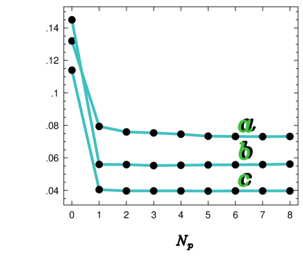
Figure 4: Standard deviation of the residuals of the $W$ fit as a function of the number of the regression parameters. Results displayed for data sets $a$ and $b$ are vertically shifted for better visibility ($const.=0.036$, $0.018$ and $0.0$ for sets $a$, $b$ and $c$, respectively

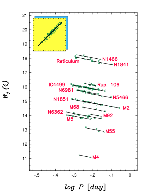
Figure 5: Observed reddening-free quantity $W=V-3.1(B-V)$ versus period. Lines show fiducial values obtained from $W_{0}$ (see the single parameter formula for data set $c$ in Table 8) after shifts with optimum distance moduli. Inset displays $W_{0}$ versus $W-d$, where $d$ is the relative distance modulus

The strong correlation of the period with $W$ for the individual cluster variables is shown in Fig. 5. As for the $M_{V}$ regression, we emphasize the importance of this correlation from the point of view of the separation of the dependence of $W$ on the period, from that of on the distance modulus.

The single parameter dependence of $W_{0}$ establishes a period-luminosity-color $(PLC)$ relation for RRab stars. The existence of this type of relation is very basic for Cepheids (e.g., Udalski et al. 1999). On the other hand, for RR Lyrae stars, to the best of our knowledge, this is the first time that the existence of this relation is exhibited and an accurate formula is given. Other works devoted to the study of the relations between the main physical and observed parameters of RR Lyrae stars have also revealed certain aspects of the $M_{V}$ and $W_{0}$ relations derived in this paper. For example, Nemec, Nemec & Lutz (1994) found $M_{V}$ – $\log P$ – [Fe/H] relations, whereas Castellani & De Santis (1994) claimed the existence of a $\log T_{\rm eff}$ – $\log P$ – $A_{B}$ (blue amplitude) relation. Sandage (1981) derived a $P$ – $L$ – $A$ relation by combining theoretical and empirical data. The results given in this paper are distinct from the above ones, because our formulae have been derived by using large data sets, which are based on the best currently available observations. In addition, our approach is completely empirical, without resorting to theoretical assumptions and few parameter (e.g., period, $B$ amplitude) searches. As a result, the formulae are more accurate. For example, the relative accuracy of the coefficient of $\log P$ in the expression for $W_{0}$ derived from data set $c$ is $2.4\%$ (for a complete error formula see Appendix A).

From the formula of Table 8 and Eq. (5), one can derive a relation for the intrinsic color index $(B-V)_{0}$. When the zero point is fitted with the one established for $(B-V)_{0}$ by KJ97, we get

$$(B-V)_{0}=0.189\log P-0.313A_{1}+0.293A_{3}+0.460\hskip 2.84526pt.$$ (6)

A more conservative expression is obtained if the two parameter counterpart of Eq. (5) in conjunction with the above single parameter formula for $W_{0}$ is applied

$$(B-V)_{0}=0.209\log P-0.187A_{1}+0.453\hskip 5.69054pt.$$ (7)

This second formula is given to aid those applications in which only limited information is available on the light curves and when the goal is to compute average quantities on large samples or when one needs to combine less accurate data with the above expressions (e.g., reddening estimations). In any case, Eqs. (6) and (7) yield very similar results. By repeating the same compatibility test as for $M_{V}$, we obtain $\sigma=0.004$ mag for the standard deviation of the differences of the $(B-V)_{0}$ values obtained from these two equations. With the total $(B-V)_{0}$ range of $0.11$ mag for the RRab stars, this result implies compatibility at the 4% level. A similar conclusion can be drawn if a comparison is made between the present formulae and the one given in KJ97 (see Sect. 4 for details).

2.3 The $PLC$ relation for $V$, $I$

In KJ97 we made an attempt to derive a formula also for the other reddening-free quantity $X$, which contains $V$ and $I$. However, due to the small amount of direct cluster data available then, we combined those data with the ones for field stars, through the application of the $W_{0}$ and $(B-V)_{0}$ formulae. This is certainly not an independent derivation of the formula for $X_{0}$. Here we are in the position to give a direct estimate on $X_{0}$, based solely on cluster variables.

Because the available data are still not too extensive, we cannot make tests on independent data sets as we did in the case of $W_{0}$. By proceeding exactly in the same way as in the case of the $W$ fit, we obtain the result shown in Fig. 6 (for the list of the outliers, see Table 4). It is clear that the single parameter dependence of $X_{0}$ is very strongly suggested. For the 109 variables we get

$$X_{0}=-2.513\log P+const.\hskip 5.69054pt.$$ (8)

This expression fits the data with $\sigma=0.037$ mag. The error of the coefficient of $\log P$ is only $3\%$ (see Appendix A for the complete error formula). To exhibit the tightness of the correlation of Eq. (8) with the observations, Fig. 7 displays the fit to the variables of the individual clusters.

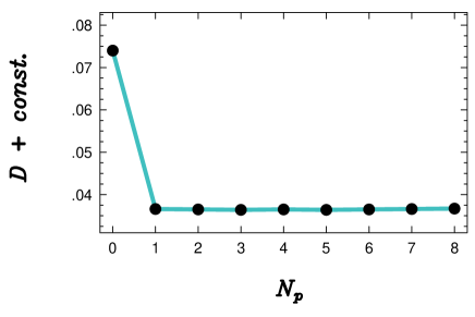
Figure 6: Standard deviation of the residuals of the $X$ fit as a function of the number of the regression parameters

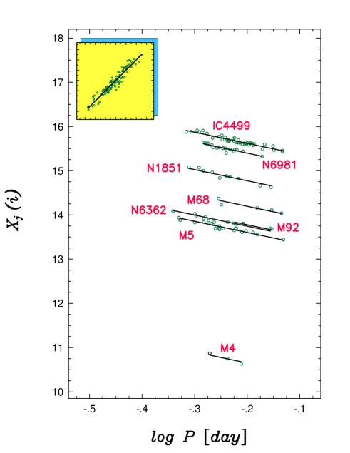
Figure 7: Observed reddening-free quantity $X=V-2.5(V-I)$ versus period. Lines show fiducial values obtained from $X_{0}$ (Eq. (8)) after shifts with optimum distance moduli. Inset displays $X_{0}$ versus $X-d$, where $d$ is the relative distance modulus

Due to the single parameter dependence of $X_{0}$, the present result is in conflict with the one given in KJ97. We recall the same facts as in the case of $W_{0}$ to explain this contradiction (see also next section for further discussion of the question related to the number of parameters in $X_{0}$ and $W_{0}$).

In the same way as in the case of $(B-V)_{0}$, the following expressions can be derived for the intrinsic color index

$$(V-I)_{0}=0.253\log P-0.388A_{1}+0.364A_{3}+0.648\hskip 2.84526pt,$$ (9)

or, by using the two parameter formula for $V_{0}$

$$(V-I)_{0}=0.278\log P-0.232A_{1}+0.640\hskip 5.69054pt.$$ (10)

Assuming standard extinction ratios (see Sect. 2), the zero points in these formulae are consistent with those of $(B\leavevmode\nobreak\ -\leavevmode\nobreak\ V)_{0}$ in the sense that they yield the same reddening with $\sigma_{\Delta E(B-V)}=0.023$ for the clusters with simultaneous $B$, $V$ and $I$ observations ($\Delta E(B-V)$ denotes the difference between the reddenings obtained from the $B-V$ and $V-I$ indices). It is suspected that at least part of this large scatter is due to zero point errors of the various color indices in the individual clusters. Color indices calculated from Eqs. (9) and (10) agree with $\sigma=0.005$ mag.

3 The problem of $T_{\rm eff}$ consistency

The derived expressions for the dereddened colors can be utilized in calculating effective temperatures. By using the stellar atmosphere models of Castelli, Gratton & Kurucz (1997), simple linear formulae can be obtained for $\log T_{\rm eff}$ as a function of the color index, gravity $\log g$ and metal abundance [M/H]. For further reference, here we repeat these formula from Kovács & Walker (1999)

$$\log T_{\rm eff} = 3.8840-0.3219(B-V)_{0}+0.0167\log g+$$ (11)

$$+ 0.0070{\rm[M/H]}\hskip 5.69054pt,$$

$$\log T_{\rm eff} = 3.9020-0.2451(V-I)_{0}+0.0099\log g+$$ (12)

$$- 0.0012{\rm[M/H]}\hskip 5.69054pt.$$

The range of validity of these formulae covers the parameter regime of cluster RRab stars, in particular, $-2.5<$[M/H]$<-0.5$. Therefore, the various temperature estimates are to be compared on the set of 383 cluster variables with $V$ observations (see Table 1). It is mentioned that while Eq. (12) fits the corresponding model values with $\sigma(\log T_{\rm eff})=0.001$, for Eq. (11) this accuracy is only $0.003$. Better fitting formulae with $(B-V)_{0}$ can be obtained by choosing narrower parameter ranges. Nevertheless, these formulae are very similar to Eq. (11), and therefore, it is not surprising that tests made with them have led to the same conclusions as the ones to be discussed below.

By using Eqs. (6) and (9), the [Fe/H] formula of JK96 and the expression given for $\log g$ by Kovács & Walker (1999), we can compute the temperature for the two color indices and compare the two estimates. The result is shown in Fig. 8. A similar correlation is obtained if Eqs. (7) and (10) are used for the color indices. The standard deviation of the $\log T_{\rm eff}$ differences is $0.0026$ mag. Considering the total range of $\approx 0.04$ mag, this size of dispersion does not seem to be small enough, although it is worth recalling the accuracy of the $T_{\rm eff}$ values obtained from the $B-V$ index (see above). More importantly, it is well known and is also clearly exhibited in Eq. (11) that $T_{\rm eff}(B-V)$ has a strong [M/H] dependence. Since this quantity is a function of $\varphi_{31}$, we would expect some dependence on this Fourier phase to be observable at least in one of the color indices. Although the effect is small, the absence of $\varphi_{31}$ is somewhat puzzling. We suspect that noise, limited [Fe/H] range of the globular clusters and delicately distributed $\varphi_{31}$ dependence between the two colors are responsible for this contradiction. In the following we show a derivation of the relation between the two color indices, which might support the above conjecture.

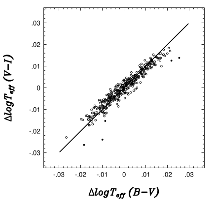
Figure 8: Relative effective temperatures calculated from color indices $B-V$ and $V-I$. Eqs. (6) and (9) are used on the full $V$ data set for cluster variables (see Table 1). Filled circles denote variables with [Fe/H]$>-0.5$. The $45^{\circ}$ line is shown for reference

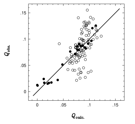
Figure 9: Observed vs. calculated reddening-free quantity $Q=V-I-1.24(B-V)$. Cluster variables are plotted by open circles, field variables by filled circles. The $45^{\circ}$ line is shown for reference

The idea is to avoid distance-dependent quantities, such as $X$, and utilize more accurate multicolor observations. It is easy to see that the quantity $Q=V-I-1.24(B-V)$ is reddening-free (assuming standard extinction ratios — see Sect. 2), independent of the distance, and enables us to use the more accurate data on field RRab stars. By employing the sample of 25 variables from KJ97, with the omission of the outlier SS Leo, the following formula is obtained

$$Q=0.477+0.397\log P-0.060\varphi_{31}\hskip 5.69054pt.$$ (13)

This expression fits the 24 variables with $\sigma=0.011$ mag. The single parameter regression contains the period and yields $\sigma=0.016$ mag. Because of the low number of data points, higher order regressions are not considered, but they all settle down at around $\sigma=0.0095$ mag. The relative errors of the regression coefficients in the above equation are 7% and 18%, for the coefficients of $\log P$ and $\varphi_{31}$, respectively.

Adding cluster variables to this sample increases the noise considerably. Fig. 9 shows the regression for this large sample. (The variables of M4 are omitted, because of their specific extinction ratios — see KJ97 and references therein.) In spite of the large scatter, this sample of 121 stars yields a very similar formula, basically with the same parameters: $Q=0.431+0.409\log P-0.051\varphi_{31}$. The significance of the two parameter formula is also very similar to the one obtained on the sample of field stars. The large scatter in this figure draws the attention to the importance of accurate photometry if more sophisticated problems, such as the one here, are studied. The majority of the outlying points in the upper left and middle right parts of the figure correspond to variables from IC4499 and N1851, respectively. Reddening could not be the cause of this scatter, because IC4499 has a relatively large reddening of $E_{B-V}=0.22$, whereas N1851 has a low one of $E_{B-V}=0.03$. The cause of the discrepancy apparent in these clusters is not known. Less accurate photometry with zero point errors, as well as peculiar extinction ratios are suspected to be the main possible agents in the systematic displacements of most of the variables of these clusters. For example, zero point errors of $\approx 0.02$ mag in the color indices might easily cause such a discrepancy.

Fig. 10 shows the improvement of the compatibility of the temperatures derived from the different colors, if Eq. (13) is used to calculate $V-I$. Although some of the metal rich stars have become ‘overcorrected’, there is a definite improvement, indicating that the predicted $\varphi_{31}$ dependence from the theoretical temperatures and the one obtained from the above, completely independent derivation agree fairly well. However, it is also noted that because $(V-I)_{0}$ is not calculated independently, the temperatures in this figure are highly correlated, which also decreases the scatter. We mention that metal rich stars are very sensitive to the contribution of $\varphi_{31}$ in the color relation $Q$. For example, switching to the relation for $Q$ obtained from the larger sample (see above), metal rich stars become even less discrepant.

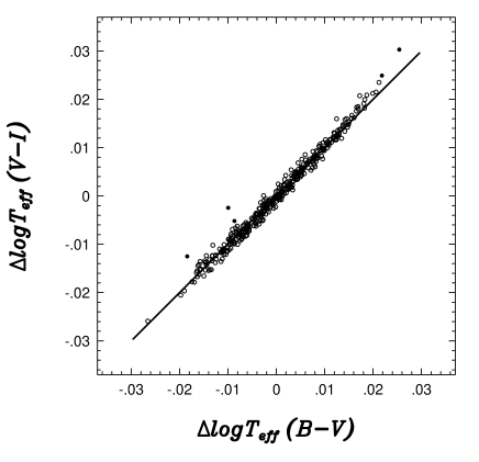
Figure 10: Relative effective temperatures calculated from color indices $B-V$ and $V-I$. Eqs. (6) and (13) are used to compute the $B-V$ and $V-I$ color indices, respectively. The full $V$ data set for cluster variables (see Table 1) is plotted. Variables with [Fe/H]$>-0.5$ are plotted by filled circles. The $45^{\circ}$ line is shown for reference

In closing this section we emphasize that the above test has been used to demonstrate only that there is a hope to derive consistent sets of equations for both color indices, but it is not claimed at this stage that we found the final formulae. The more definitive statement about this rather delicate issue may come only when additional, more accurate cluster data will become available.

4 Distance moduli, reddenings, comparison with KJ96 and KJ97

Average values and standard deviations of $E_{B-V}$ and those of the various distance moduli are summarized in Table 9. Abundances — computed by the formula of JK96 — are also listed for completeness. Except for the calculation of [Fe/H], data sets without the outliers, as given in Table 4 were used. For [Fe/H] we employed the full set $C$ of Table 3. The outliers (which were discrepant in respect of the average cluster [Fe/H] values) are listed in the note to Table 9. These variables have been omitted in the calculation of the averages and standard deviations. Reddening has always been calculated from the $B$ and $V$ colors and not from the less extensive (and probably also less accurate) $I$ data. Because of the still debated issue of the luminosity of the RR Lyrae stars, we show only relative distances, all normalized to zero for IC4499.

Table 9: Metallicities, reddenings and relative distance moduli

Cluster	$\langle$[Fe/H]$\rangle$	$\sigma($[Fe/H]$)$	$\langle E_{B-V}\rangle$	$\sigma(E_{B-V})$	$\langle\tilde{d}_{V}\rangle$	$\sigma(\tilde{d}_{V})$	$\langle d_{W}\rangle$	$\sigma(d_{W})$	$\langle d_{X}\rangle$	$\sigma(d_{X})$
M2	$-1.43$	0.15	0.011	0.008	$-1.61$	0.02	$-0.99$	0.04	—	—
M3	$-1.36$	0.16	—	—	$-2.04$	0.03	—	—	—	—
M4	$-1.03$	0.07	0.339	0.038	$-5.69$	0.02	$-5.15$	0.02	$-5.30$	0.04
M5	$-1.22$	0.13	0.065	0.020	$-2.64$	0.04	$-2.16$	0.05	$-2.02$	0.04
M9	$-1.75$	0.14	—	—	$-1.44$	0.04	—	—	—	—
M55	$-1.57$	0.23	0.092	0.029	$-3.21$	0.04	$-2.83$	0.08	—	—
M68	$-1.76$	0.09	0.034	0.007	$-1.98$	0.04	$-1.41$	0.05	$-1.42$	0.05
M92	$-1.98$	0.06	0.012	0.007	$-2.45$	0.06	$-1.81$	0.02	$-1.84$	0.03
M107	$-0.96$	0.17	—	—	$-2.01$	0.06	—	—	—	—
NGC1851	$-1.19$	0.09	0.034	0.015	$-1.57$	0.03	$-1.01$	0.05	$-0.85$	0.04
NGC5466	$-1.66$	0.09	$-0.013$	0.014	$-1.08$	0.02	$-0.37$	0.03	—	—
NGC6362	$-0.98$	0.15	0.073	0.008	$-2.42$	0.04	$-1.97$	0.04	$-1.88$	0.03
NGC6981	$-1.31$	0.14	0.052	0.010	$-0.81$	0.03	$-0.30$	0.03	$-0.22$	0.03
IC4499	$-1.46$	0.19	0.217	0.013	$0.00$	0.04	$0.00$	0.04	$0.00$	0.04
Rup. 106	$-1.57$	0.28	0.158	0.014	$0.08$	0.04	$0.27$	0.04	—	—
$\omega$ Cen	$-1.54$	0.09	—	—	$-2.99$	0.05	—	—	—	—
NGC 1466	$-1.56$	0.27	0.060	0.010	$1.66$	0.04	$2.17$	0.04	—	—
NGC 1841	$-1.71$	0.14	0.145	0.014	$1.74$	0.04	$1.94$	0.05	—	—
Reticulum	$-1.45$	0.12	0.024	0.012	$1.40$	0.04	$1.99$	0.04	—	—
Sculptor	$-1.51$	0.25	—	—	$2.48$	0.05	—	—	—	—

• • • $\tilde{d}_{V}$ denotes reddened distance moduli, calculated from color $V$

    • $R_{V}=4.1$ and $R_{I}=3.3$ are used in the calculation of the distance moduli for M4

    • $\sigma(E_{B-V})=\sigma[(B-V)_{obs}-(B-V)_{0}]$, i.e., $\sigma(E_{B-V})$ contains both observational noise and contribution from reddening inhomogeneities

    • Zero points of the distance moduli are set to yield zero distance moduli for IC4499

    • Outliers with respect to the average cluster abundances and dispersions (derived [Fe/H] values are shown in parentheses): M2: V708($-0.14$); M3: V50($-1.91$), V106($-0.76$); M5: V6($-1.71$), V38($-0.58$), V56($-0.66$), V963($0.60$); M107: V12($-0.06$); N1851: V8($-1.63$), V20($-0.66$); N6362: V361($-0.41$); N6981: V297($-0.86$); IC4499: V30($-0.32$), V61($-0.73$), V72($-0.78$); $\omega$ Cen: V77($-1.21$), V88($-1.16$), V114($-0.80$), V137($-2.06$), V146($-1.07$), V154($-1.15$); Rup. 106: V5($-0.58$)

As we have already noted in our former papers, and is also clearly seen in Table 9, in some clusters the derived metallicity values exhibit considerable scatter. It is worth noting that recent spectroscopic analysis of the horizontal branch stars in M13 by Behr et al. (1999) also revealed substantial inhomogeneities. It is seen that most of the clusters have metallicities around $-1.5$ and there are only a few with [Fe/H]_∼^>$-1.0$ or [Fe/H]_∼^<$-1.9$. This distribution of [Fe/H] signals some warning in respect of the unbiased coverage of the possible evolutionary stages by the present sample. Specifically, one should exercise some caution in extrapolating the results of this paper to more metal abundant variables, such as the ones observed in the Galactic field.

Reddening could also be inhomogeneous, with an observed overall standard deviation of $\approx 0.014$ mag. Because observational noise is also present in the data, the true dispersion of $E_{B-V}$ is smaller than this formal value. A more accurate upper limit on the overall reddening dispersion can be derived with the aid of some basic equations connecting various noise properties. Denoting the standard deviations of the residuals of the $V_{0}$, $W_{0}$ and $(B-V)_{0}$ regressions by $\sigma(V)$, $\sigma(W)$ and $\sigma(B-V)$ respectively, it is easy to see that the following relations hold for these quantities

$$\sigma^{2}(V) = \sigma^{2}_{V}+R^{2}_{V}\sigma^{2}_{E}\hskip 5.69054pt,$$ (14)

$$\sigma^{2}(W) = (1+R_{V})^{2}\sigma^{2}_{V}+R_{V}^{2}\sigma^{2}_{B}-$$ (15)

$$- 2R_{V}(1+R_{V})K^{\star}\hskip 5.69054pt,$$

$$\sigma^{2}(B-V) = \sigma^{2}_{V}+\sigma^{2}_{B}+\sigma^{2}_{E}-2K^{\star}\hskip 5.69054pt,$$ (16)

where $K^{\star}=K\sigma_{V}\sigma_{B}$, $K$ and the other quantities have the same meaning as in Eq. (3). Elimination of $\sigma_{V}$ and $\sigma_{B}$ from these equations results in the following expression for $\sigma_{E}$

$$\sigma^{2}_{E} = {(1+2R_{V})\sigma^{2}(V)+R^{2}_{V}\sigma^{2}(B-V)-\sigma^{2}(W)\over 2R^{2}_{V}(1+R_{V})}-$$ (17)

$$- {K^{\star}\over R_{V}(1+R_{V})}\hskip 5.69054pt.$$

Although the correlation coefficient $K$ is not known, it can be safely assumed that it is positive (e.g., random background contamination influences both colors in a similar way). From Tables 6 and 8 we get $\sigma(V)=0.040$ and $\sigma(W)=0.041$. A direct fit to the observed $(B-V)$ values yields $\sigma(B-V)=0.014$. These values and the $K^{\star}>0$ condition leads to the upper limit of $0.012$ mag for $\sigma_{E}$. This constraint yields also a lower limit for $\sigma_{V}$. From Eq. (14) we get $\sigma_{V}>0.018$ mag. (This latter quantity is very sensitive to the value of $\sigma_{E}$. The value quoted was obtained from the formal value of $\sigma_{E}=0.0115$.) These limits are average values, deviations from them might occur in the individual clusters.

In comparing the $d_{W}$ and $d_{X}$ distance moduli, we see that substantial differences might exist between them. Unfortunately, these true distance moduli derived from medium wavelength optical photometry are rather sensitive to zero point errors. Indeed, if the zero points are changed by $\Delta V$, $\Delta B$ and $\Delta I$, assuming standard extinction ratios, the difference between the derived distance moduli from $W$ and $X$ becomes $d_{W}-d_{X}=5.5\Delta V-3.1\Delta B-2.5\Delta I$. With the commonly admitted zero point errors of $0.01$ mag, it is very easy to accumulate a difference of $0.1$ mag between the two types of distance moduli.

As we have already noted at the beginning, the present data sets are much more extensive then the ones used in our previous studies. Therefore, it is a matter of interest to check the difference between the old and new formulae. For the following reasons, in this comparison we restrict ourselves only to $M_{V}$ and $(B-V)_{0}$. For the $V-I$ index the data are still limited and the result of the comparison depends on whether we rely solely on the fit obtained from cluster variables, or incorporate the data available on field stars (as it was done in KJ97). Therefore, it is not possible to make a consistent comparison. For $(V-K)_{0}$, there are only field data available with sufficient accuracy. In addition, because of their limited number, the result depends on the selection of the outliers. Therefore, we do not deal with this color either.

The comparison for $M_{V}$ and $(B-V)_{0}$ is made on the same large data set of 500 stars which was already employed for similar tests in Sect. 2. The results are displayed in Fig. 11. We can conclude that both quantities were reasonably well approximated already in KJ96 and KJ97.

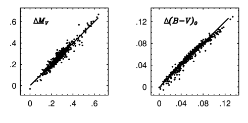
Figure 11: Comparison of the empirical relations derived in this paper and those given by KJ96 and KJ97. For the employed relations see the three parameter formula for data set $C$ in Table 6 and Eq. (6). Vertical axes: this paper; horizontal axes: KJ96 & KJ97. The zero points are arbitrary. The $45^{\circ}$ lines are plotted for reference

5 Discussion and conclusions

In an effort to utilize the steadily increasing number of light curves accumulated during the various photometric surveys and ccd works on individual clusters, we revisited the problem of absolute magnitude and intrinsic color calibrations in terms of the Fourier parameters of the light curves in $V$ color. The amount of data used in this paper is more than a factor of two larger than the one used in our similar studies conducted a few years ago. The increase of the data base is beneficial for the following reasons: (i) the larger data sets enable us to derive statistically more significant relations; (ii) the number of parameters entering in the finally adopted formulae does not depend on the omission of the outliers, whose treatment could be a delicate problem in the case of small sample size; (iii) with the larger number of variables, it is hoped that there is a better representation of the various evolutionary stages and also physical parameters, most importantly luminosity levels and abundances. It is this latter point which is perhaps the most crucial in the applicability of the derived formulae. In the present sample most of the data concentrate around [Fe/H]$\approx-1.5$ and only a few clusters occupy the extremes close to [Fe/H]$=-1.0$ and $-2.0$. Therefore, some degree of caution is necessary when extrapolating the present results to variables with different metallicities, and especially beyond the high metallicity end (e.g., metal rich Galactic field variables).

The effective temperatures calculated from the expressions for $B-V$ and $V-I$ agree with $\sigma(\Delta\log T_{\rm eff})=0.003$. The lack of higher level compatibility is due to the absence of phase dependence in our formulae which is required by the explicit [Fe/H] dependence in $T_{\rm eff}$, predicted by stellar atmosphere models and by our formulae derived earlier for [Fe/H]. The test presented in Sect. 3 suggests that the limited [Fe/H] coverage of the cluster data together with the still sufficiently high observational noise in the cluster data, are probably the main sources of the lack of better agreement between the various temperature estimates.

For the absolute magnitude $M_{V}$, a highly significant three parameter formula has been derived with period $P$ and Fourier amplitudes $A_{1}$ and $A_{3}$. There is also an indication for the presence of the Fourier phase $\varphi_{51}$, although with a much lower significance. In certain applications (e.g., in computing averages on large representative samples) there are very little differences between the high and low parameter formulae. In the case of less accurate data, one can use even the two parameter formula as it is given in Table 6.

For the reddening-free quantities $W=V-R_{V}(B-V)$ and $X=V-R_{I}(V-I)$ we obtained basically single parameter formulae. Although these $PLC$ relations are rather tight and well defined, it is worth remembering that this is not entirely consistent with the requirement posed by stellar atmosphere models (see above).

Although the accurate value of the observational noise is not known, from the standard deviations of the residuals of the various regressions we may have estimates both on the observational noise and also on the dispersion of the reddening. For the latter quantity an upper limit was obtained, with $\sigma_{E}<0.012$ mag. This value puts a lower limit on the average observational noise, giving $\sigma_{V}>0.018$ mag. From this result and the fit of the reddening- and distance-free quantity $Q=V-I-1.24(B-V)$ we can conclude that although the presently available ccd photometric data on cluster variables allow us to derive more accurate empirical relations than ever before, the average colors (mostly due to crowded field effects) may still be not accurate enough to address more sophisticated questions, such as the higher level compatibility of the temperature estimates obtained from various colors.

From the point of view of applicability, it is worth mentioning that the estimated probability that the present formulae give incorrect (i.e., $\approx 3\sigma$ discrepant) result is less than 5% (assuming that they are employed on RRab stars with stable light curves, which cover approximately the same [Fe/H] range as the ones in our sample). The formal statistical accuracy of the individual estimates are better than $\sigma(M_{V})\approx 0.01$ and $\sigma(W_{0})\approx\sigma(X_{0})\approx 0.005$. Therefore, these formulae are suitable (under the condition just mentioned) for the accurate calculation of relative absolute magnitudes, distance moduli and reddenings. When combined with stellar atmosphere models, the formulae are very useful in mapping the instability strip (Jurcsik 1998) and comparing with the predictions of pulsation models (Kolláth, Buchler & Feuchtinger 2000). Further improvement of the formulae requires more accurate cluster data together with a better sampling at the low and high metallicity limits. Considering the steady progress in cluster photometry, we think that these goals are reachable in the very near future.

Appendix A

In the following we give a summary of the statistical error formulae for $M_{V}$, $W_{0}$ and $X_{0}$. Starting with the two parameter expression for $M_{V}$ (see the 3rd row of Table 6), assuming that the period is error-free, the variance can be written in the following form

$$\sigma^{2}_{M_{V}}=0.805^{2}\sigma^{2}_{A_{1}}+\sigma^{2}\sum^{3}_{i,j=1}K_{ij}p_{i}p_{j}\hskip 5.69054pt,$$ (18)

where $\sigma=0.0416$, $p_{1}=1$, $p_{2}=\log P+0.22488$, $p_{3}=A_{1}-0.32161$, and the symmetric correlation matrix $K_{ij}$ is given in Table A.1. We see that the $K_{1i}$ elements are zero (lower than $10^{-5}$), because the corresponding sample averages have been subtracted from the parameters. In the same way as above, for the three parameter expression of $M_{V}$ (see the 4th row of Table 6), we get

$$\sigma^{2}_{M_{V}}=1.158^{2}\sigma^{2}_{A_{1}}+0.821^{2}\sigma^{2}_{A_{3}}+\sigma^{2}\sum^{4}_{i,j=1}K_{ij}p_{i}p_{j}\hskip 5.69054pt,$$ (19)

where $\sigma=0.0399$, $p_{1}$ — $p_{3}$ are the same as above, $p_{4}=A_{3}-0.09926$. Table A.2 displays the correlation matrix.

Table 10: Correlation coefficients $K_{ij}$ in the error formula Eq. (A.1)

i	j	$K_{ij}$	i	j	$K_{ij}$
1	1	$0.00273$	2	2	$1.63537$
1	2	$0.00000$	2	3	$0.74685$
1	3	$0.00000$	3	3	$0.78466$

Table 11: Correlation coefficients $K_{ij}$ in the error formula Eq. (A.2)

i	j	$K_{ij}$	i	j	$K_{ij}$
1	1	$0.00273$	2	3	$1.00646$
1	2	$0.00000$	2	4	$-0.61883$
1	3	$0.00000$	3	3	$2.99961$
1	4	$0.00000$	3	4	$-5.27980$
2	2	$1.66580$	4	4	$12.58549$

Because $W_{0}$ and $X_{0}$ depend only on the period, their error formulae are simpler

$$\sigma^{2}_{W_{0}} = 0.0405^{2}[0.00581+2.113(\log P+0.22395)^{2}]\hskip 1.42262pt,$$ (20)

$$\sigma^{2}_{X_{0}} = 0.0366^{2}[0.00917+4.311(\log P+0.23329)^{2}]\hskip 1.42262pt.$$ (21)

References

- (1) Behr B. B., Cohen J. G., McCarthy J. K. & Djorgovski, S. G., 1999, ApJ (Letters) 517, L135
- (2) Bono G., Caputo F. & Stellingwerf R. F., 1995, ApJS 99, 263
- (3) Cardielli J. A., Clayton G. C. & Mathis J. S., 1989, ApJ 345, 245
- (4) Castellani V. & De Santis R., 1994, ApJ 430, 624
- (5) Castelli F., Gratton R. G. & Kurucz R. L., 1997, A&A 318, 841
- (6) Clement C. M. & Shelton I., 1997, AJ 113, 1711
- (7) Clement C. M. & Shelton I., 1999, AJ 118, 453
- (8) Corwin T. M., Carney B. W. & Nifong B. G., 1999, AJ 118, 2875
- (9) Feast M. W., 1999, PASP 111, 775
- (10) Jurcsik J., 1998, A&A 333, 571
- (11) Jurcsik J. & Kovács G., 1996, A&A 312, 111 (JK96)
- (12) Kaluzny J., Krzemiński W. & Mazur B. 1995a, AJ 110, 2206
- (13) Kaluzny J., Kubiak M., Szymański M., Udalski A., Krzeminśki W. & Mateo, M. 1995b, A&AS 112, 407
- (14) Kaluzny J., Kubiak M., Szymański M., Udalski A., Krzemiński W. & Mateo M., 1997, A&AS 125, 343
- (15) Kaluzny J., Hilditch R. W., Clement C. M. & Rucinski S. M., 1998, MNRAS 296, 347
- (16) Kaluzny J., Olech A., Thompson I., Pych W., Krzemiński W. & Schwarzenberg-Czerny A., 2000, A&AS 143, 215
- (17) Kanbur S. M., Mariani H. & Iono D., 2000, preprint
- (18) Kolláth Z., Buchler J. R. & Feuchtinger M., 2000, ApJ 540, 468
- (19) Kovács G., 2000, A&A 363, L1
- (20) Kovács G. & Jurcsik, J., 1996, ApJ (Letters) 466, L17 (KJ96)
- (21) Kovács G. & Jurcsik J., 1997, A&A 322, 218 (KJ97)
- (22) Kovács G. & Kanbur S. M., 1998, M.N.R.A.S. 295, 834.
- (23) Kovács G. & Walker A.R., 1999, ApJ 512, 271
- (24) Lee J-W & Carney B. W., 1999, AJ 117, 2868
- (25) Liu T. & Janes K.A., 1990, ApJ, 354, 273
- (26) Nemec J. M., Linnell Nemec A. F. & Lutz T. E., 1994, AJ 108, 222
- (27) Olech A., Kaluzny J., Thompson I. B., Pych W., Krzemiński W. & Schwarzenberg-Czerny A., 1999, AJ 118, 442
- (28) Preston G. W., 1959, ApJ 130, 507
- (29) Sachs L., 1982, Applied Statistics, a Handbook of Techniques, Springer-Verlag New York Inc.
- (30) Sandage A., 1981, ApJ 248, 161
- (31) Simon N. R. & Teays T. J., 1982, ApJ 261, 586
- (32) Stanek K. Z., Kaluzny J., Wysocka A. & Thompson I., 2000, Acta Astr. 50, 191
- (33) Udalski A., Szymański M., Kubiak M., Pietrzyński G., Soszyński I., Woźniak P. & Żebruń K., 1999, Acta Astron. 49, 201
- (34) Walker A. R., 1990, AJ 100, 1532
- (35) Walker A. R., 1992a, AJ 103, 1166
- (36) Walker A. R., 1992b, AJ 104, 1395
- (37) Walker A. R., 1994, AJ 108, 555
- (38) Walker A. R., 1998, AJ 116, 220
- (39) Walker A. R. & Nemec J. M. 1996, AJ 112, 2026