High Sensitivity, High Spectral Resolution, Mid-infrared Spectroscopy

Abstract

We broadly discuss mid-infrared spectroscopy and detail our new high spectral resolution instrument, the Texas Echelon-cross-Echelle Spectrograph (TEXES).

University of Texas Astronomy Department, Austin, TX 78712

1. Introduction

In Bob Tull’s design and construction of high resolution, optical spectrographs at McDonald Observatory, he has had the advantage of being able to crawl around inside his spectrograph to see how the instrument is behaving. That advantage, along with careful design and great experience, has allowed him to make spectrographs like 2dcoude: R$\equiv{\lambda\over{\Delta\lambda}}$ up to 250,000 or R=60,000 and complete optical coverage in two settings (Tull et al. 1995). We have built a spectrograph that does not quite equal Bob’s work in terms of maximum spectral resolution or fractional wavelength coverage, but operates at 20 times longer wavelength with 60 times fewer pixels. It can rightfully be called the first true high spectral resolution grating spectrograph for the mid-infrared (MIR).

The MIR, here defined as 5 $\mu$m$<\lambda<$25 $\mu$m, is somewhat exotic. Section 2 gives some background about observing near 10 $\mu$m. Section 3 describes MIR spectral features, past results, and present and future instruments. In Section 4 we discuss methods of obtaining R=100,000 at 10 $\mu$m. Finally, in Section 5, we describe our instrument, TEXES, in more detail and present some preliminary results.

2. Observing in the MIR

Ground-based MIR astronomy is predominantly limited by the atmosphere and background radiation. The Earth’s atmosphere limits observations to spectral regions, windows, where terrestrial molecules do not absorb light from space. More importantly, molecules that absorb photons also emit photons, contributing to the background photon rate. In most cases, photon noise from the background emission is the limiting factor in the sensitivity of MIR instruments.

Figure 1 shows the MIR atmospheric transmission from Mauna Kea on a dry night.

Figure 1.: Transmission through the Earth’s atmosphere based on a model calculation. Some of the major molecular absorbers are identified in the text.

The dominant absorbers are H₂O (5.5-7.5 $\mu$m, 17-30 $\mu$m), CO₂ (13.5-16.5 $\mu$m), and O₃ (9.5-10 $\mu$m). Water is particularly devastating because the lines form low in Earth’s atmosphere and are substantially pressure-broadened. Observing from high, dry sites substantially improves the transmission (Figure 2)

Figure 2.: Models of the terrestrial transmission for elevations of 14,000 feet (solid line) and 7,000 feet (dotted line). The far wings of water lines are responsible for the reduction in the peak transmission at lower altitudes.

The background photon rate is given by

$$N_{\gamma}=2.36\times 10^{-11}{\epsilon B_{\nu}(T)\over h\nu}A\,\,\,{\rm[photons/s/Hz/arcsec^{2}]}$$

where $\epsilon$ is the sky+telescope+instrument emissivity, $B_{\nu}(T)$ is the Planck function, $A$ is the telescope area, $h\nu$ is the energy of the photon, and the numerical factor converts the solid angle to $arcsec^{2}$. A typical number for a 3 meter telescope with $\epsilon=0.1$ would be 5$\times 10^{9}$ photons s^-1 $\mu$m^-1 arcsec^-2 or a background of approximately -2.7 mag arcsec^-2. Note that a cooled, space telescope will have orders of magnitude improvement in sensitivity.

3. MIR Spectroscopy

MIR spectral features can be loosely divided into three categories: solid features, ionic lines, and molecular rotation-vibration transitions. Each of these classes probes a different environment and is best observed with different spectral resolution. Solid features include dust grains, ices, and polycyclic aromatic hydrocarbons (PAHs). The broad nature of these features suggest observations at low spectral resolution, R$\sim$100 to 1000. Ionic and atomic spectral lines, for example from HII regions, external galaxies, or shock excited regions, require higher resolving power: R$\sim$1000 to 10,000. Molecular transitions are often associated with cold interstellar gas or stellar photospheres. Observing molecular lines requires high spectral resolution: R$\sim$10,000 to 100,000.

Most molecular transitions in the MIR are rotation-vibration bands. Therefore, many lines, each arising from a different rotational energy level of the same molecule, are closely spaced in frequency. In addition, isotopic transitions and transitions involving higher vibrational states may also overlap in frequency. With sufficient spectral coverage one can simultaneously observe transitions with a range of sensitivity to temperature and density, providing a consistent data set with multiple constraints.

Table 1 lists commonly observed molecules in the MIR. Molecules without an electric dipole, H₂, CH₄, and C₂H₂, are unobservable with radio telescopes.

Table 1.: Important MIR molecules

Molecule	Comments
H2	pure rotational lines throughout MIR
H2O	pure rotation and ro-vibrational lines throughout MIR
CH4	band at 7.7 $\mu$m
C2H2	band at 13.7 $\mu$m
HCN	band at 14.0 $\mu$m
C2H6	bands at 12.2
SiO	band at 8.1 $\mu$m
NH3	bands at 10 $\mu$m

Table 2 provides a non-exhaustive list of some past, present, and future MIR spectrographs along with their resolving power. Clearly, very few instruments are designed to concentrate on MIR molecular spectroscopy. Unfortunately, infrared space telescopes, although extremely sensitive, are not equipped with high resolution spectrographs primarily because of weight and size limitations.

Table 2.: Some Past, Present and Future MIR Spectrographs

Instrument	Resolving Power	Telescope
FTS	50,000	KPNO (past)
Irshell	10,000	IRTF and ESO (past)
ISO SWS	2,000 (10,000)	ISO satellite (past)
Keck LWS	1,000	Keck (present)
Celeste	10,000	KPNO and IRTF (present)
HIPWAC	1,000,000	IRTF (present)
TEXES	100,000	IRTF (present)
COMICS	1-5,000	Suburu (present)
Michelle	1-30,000	UKIRT and Gemini (future)
VISIR	1-30,000	VLT (future)
SIRTF IRS	600	SIRTF satellite (future)

MIR spectroscopy definitely advanced in importance with the success of the Infrared Space Observatory (ISO). ISO’s Short Wavelength Spectrometer (SWS; de Graauw et al. 1996), provided many beautiful data sets throughout the MIR with a resolving power $\sim$2000. Figures 3 and 4 present examples of SWS data. Figure 3 shows solid features and some ionic lines from evolved stars (Molster et al. 1996).

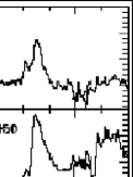
Figure 3.: Taken from Molster et al. (1996) showing the MIR spectra of several evolved stars. The broad features are PAHs. The sharp lines in the bottom panel are ionic emission lines.

Figure 4 shows Jupiter in the MIR along with a model spectrum and identification of molecular features (Encrenaz et al. 1996).

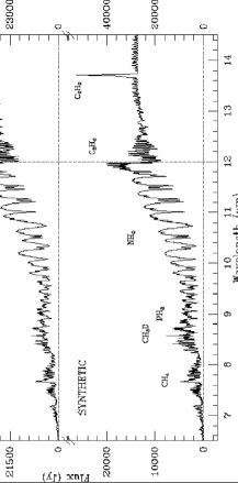
Figure 4.: SWS spectrum of Jupiter plus model identifying some molecular bands. (Encrenaz et al. 1996).

Both figures show the tremendous signal-to-noise and wavelength coverage achieved by the SWS. However, it is important to note that with the SWS spectral resolution, narrow features such as the C₂H₂ Q-branch at 729 cm^-1 are totally blended together.

Figure 5 is a figure taken from Evans et al. (1991) showing the observations of the C₂H₂ Q-branch in absorption toward IRc2 in Orion.

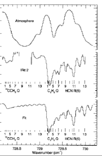
Figure 5.: Molecular absorption toward IRc2 at the C₂H₂ Q-branch along with observation of the atmosphere for comparison. Note the number of lines observed with a single setting.

These observations, taken from the ground with Irshell (Lacy et al. 1989), demonstrate the information available with higher resolution and the difficulty of observing through the Earth’s atmosphere (note the top trace showing an observation of the atmospheric absorption).

4. High Spectral Resolution

There are three major benefits to using high spectral resolution: First, resolving the Earth’s atmospheric lines makes observing between the lines practical. Furthermore, correcting for the atmospheric lines becomes easier. Second, when the line width matches the resolution of an instrument, the instrument’s sensitivity to that line is at a maximum. Finally, if the line is fully resolved, line profile information becomes available for modeling and analysis.

Several types of instrument can achieve R=100,000 in the MIR, each with advantages. We will now discuss three methods to illustrate our decision in favor of a grating spectrograph. We will not include coherent systems, such as heterodyne spectrometers, which easily reach the resolution requirement, but have limited sensitivity, spatial coverage, and spectral coverage (e.g. Betz 1980).

Fourier transform spectrometers (FTS), such as the one used at KPNO (Hall et al. 1979), operate by sampling the Fourier transform of the spectrum over a range of phase delays. For a more detailed discussion of an FTS, see Hinkle (this volume). In the basic design, a Michelson interferometer, a beamsplitter divides the light between two separate arms, the reference and the scanning arm, and recombines before reaching the detector. To achieve R=100,000 at 10 $\mu$m, the scanning mirror must travel at least 0.5 m. The detector records the intensity as a function of the phase delay and the resulting spectrum is recovered in software. If used with an array detector, an FTS will simultaneously sample the spectrum of all points in the field-of-view (Maillard 1995). Because the FTS samples the entire bandpass at all times, the noise also comes from the entire bandpass and fluctuations in the sky background will affect the entire spectrum. An FTS is most efficient when seeking extended wavelength coverage over an extended object.

A Fabry-Perot (FP) is a scanning monochromator which measures spectral elements sequentially. With an array detector, it can also simultaneously record spectra of an extended object, albeit with spectral shifts across the field. To achieve R=100,000 requires multiple, cryogenic FP etalons. Assuming a high plate finesse of 50, the spacing must be 1 cm and the free spectral range will be 0.5 cm^-1, requiring at least two additional elements, such as a cryogenic FP and a narrow-band filter, to isolate the orders. As with the FTS, an FP is subject to noise from sky fluctuations. An FP is most efficient if observing a single line over an extended object.

A diffraction grating disperses light in a single dimension. With a detector array, a grating spectrograph will sample a continuous spectrum along with one spatial dimension defined by the entrance slit. To achieve R=100,000 at 10 $\mu$m requires a grating $\geq$0.5 m long, as will be discussed below. A grating is most efficient when observing a point source over an extended spectral range.

5. TEXES

Because our science involves molecular rotation-vibration lines, mostly in point sources, we chose to design and build a grating spectrograph, the Texas Echelon-Cross-Echelle Spectrograph or TEXES. TEXES operates from 5 to 25 $\mu$m with multiple spectroscopic modes: R$\approx$100,000 in a cross-dispersed format; R$\approx$15,000 in single order; and R$\approx$3,000 in single order. It is available to the community on a collaborative basis. Recent observing runs at the McDonald 2.7 m telescope and NASA’s 3 m Infrared Telescope Facility (IRTF) have demonstrated the capabilities of the instrument. TEXES also serves as a test-bed for construction of our SOFIA instrument, EXES.

The heart of TEXES is an echelon grating, a steeply blazed, coarsely ruled, diffraction grating (Michelson 1898). For a reflection grating, the grating equation is

$$m\,\lambda=2\,d\,(sin\,\alpha+sin\,\beta)$$

where $m$ is the grating order, $\lambda$ is the wavelength of interest, $d$ is the groove spacing, and $\alpha$ and $\beta$ are the angles of incidence and diffraction, respectively. The theoretical resolving power in the diffraction limited case with $\alpha\approx\beta\equiv\theta$ is

$$R={2\,L\,sin\,\theta\over\lambda}$$

where $L$ is the length of the grating. For high resolution within a confined volume, both the angle of incidence and the length of the grating must be large.

Our echelon grating is a single piece of diamond-machined aluminum. It is 36 inches long with a 3.4 inch square cross-section. The angle of incidence is 84.3^∘. The groove spacing is 0.3 inch or, in more familiar terms, 0.133 lines/mm. The grating was manufactured by Hyperfine, Inc of Boulder, Colorado (Bach, Bach, & Bach 2000). For images of the slightly longer EXES grating, see

$$http://nene.as.utexas.edu/exes/epo/figures/scifigs.html.$$

The echelon design is very appropriate for a MIR instrument. Since the groove spacing is so coarse, we operate in 1500^th order at 10 $\mu$m with a limited free spectral range, 0.66214 cm^-1. However, our MIR detector array, with only 256 $\times$ 256 pixels, is small enough that orders overfill the array longward of 11 $\mu$m. In theory, the diffraction limited resolving power of our instrument is R=180,000. Because working at the diffraction limit is difficult to achieve and inefficient due to light loss at the entrance slit, we typically operate at R$\approx$75,000.

We have conducted some laboratory tests to investigate the performance of the echelon. Using a room temperature gas cell, we create an emission line spectrum. Figure 6 shows gas cell spectra of CH₄ and C₂H₂ at 7.7 $\mu$m and 13.7 $\mu$m.

Figure 6.: Laboratory gas cell spectra of CH₄ and C₂H₂. Each spectrum contains several orders that have been pieced together in the 1D format. Tick marks indicate the line frequencies. At the CH₄ setting, we have continuous wavelength coverage. while at the C₂H₂ setting, the orders are larger than the detector, causing the gaps in the spectrum.

The C₂H₂ spectra includes the region shown in Figure 5 observed with Irshell by Evans et al. (1991). With TEXES, it is easy to separate the individual Q-branch lines. From these spectra, we find deviations from Gaussian line profiles at 7.7 $\mu$m and Gaussian profiles at 13.7 $\mu$m (Figure 7).

Figure 7.: The results of Gaussian fits to relatively isolated lines of CH₄ and C₂H₂. At the shorter wavelength, there is a wing to the spectral lines while the shape is very Gaussian at longer wavelengths.

Typical FWHM for each wavelength demonstrates R=75,000 in both cases.

TEXES’s initial observing run was on the McDonald Observatory 2.7 m telescope in February, 2000. We had 8 nights for a combination of engineering and science projects. Figure 8 shows a high resolution, cross-dispersed spectrum of Jupiter with numerous C₂H₆ lines in emission and the same data summed along the slit and reorganized in a 1D format.

Figure 8.: A 2D echellogram showing C₂H₆ emission from Jupiter’s stratosphere observed with TEXES at McDonald Observatory. The integration time was a few minutes on source with equal time on sky. In the greyscale image, black represents the most intense emission, grey comes mostly from Jupiter’s continuum, and the unilluminated portions of the detector are white. The 1D plot shows the sum along the slit for each order with three orders per panel. In both cases, frequency increases down and to the left (wavelength increases up and to the right). The arrows indicate the relationship between the two presentations. At this wavelength, 12 $\mu$m, orders are larger than the detector and we do not get complete wavelength coverage, as seen by the regions where intensity goes to zero.

We have subsequently had about 12 clear nights on NASA’s IRTF. With a larger, infrared-optimized telescope at about twice the altitude, we have had a significant improvement in our signal-to-noise of roughly a factor of 10. Projects that were awarded time include: searching for H₂ pure rotational lines in Uranus, planetary nebulae, and young stellar objects; examining C₂H₂ and HCN absorption toward massive star formation regions, looking at Jupiter and Saturn in a variety of molecules, and investigating stellar Mg I emission and H₂O absorption for a range of spectral types. Detailed results of these projects are awaiting complete data reduction and will be published elsewhere, but one preliminary observational result illustrates TEXES’s performance.

Two Mg I lines near 12 $\mu$m (811.578 and 818.058 cm^-1) were found in the Sun to be Zeeman sensitive (Brault & Noyes 1983). These photospheric emission lines have been modeled by Carlsson, Rutten, & Shchukina (1992) and are still used for solar magnetic field studies (Moran et al. 2000). Because the Zeeman splitting increases with wavelength relative to Doppler broadening, these MIR lines hold great potential for measurement of stellar magnetic fields.

Jennings et al. (1986) observed two stars, $\alpha$ Ori and $\alpha$ Tau, with the KPNO 4 m telescope and FTS searching for the 811.578 cm^-1 line. The resolving power selected was 50,000 with a wavelength coverage of 2 cm^-1. Several hours of integration produced a firm detection in $\alpha$ Ori and a probable detection in $\alpha$ Tau, both in absorption. Later it was recognized that the absorption in $\alpha$ Ori was from H₂O (Jennings & Sada 1998).

In Figure 9 we show a spectrum of $\alpha$ Tau obtained at the IRTF with TEXES. The spectral resolution is 75,000 (all lines resolved) with a coverage of almost 6 cm^-1. This is a single nod pair with total integration time of 4 seconds.

Figure 9.: TEXES spectrum of $\alpha$ Tau taken at the IRTF. The data (heavy line) are the result of differencing a single image pair and using our pipeline data reduction program. For reference, we show a sunspot spectrum (lower line; offset by -0.35 in the figure) and a solar penumbra plus terrestrial atmosphere spectrum (upper line; offset by +0.75) taken from the KPNO Sunspot Atlas (Wallace, Livingston, & Bernath 1994). In the penumbra spectrum, the Mg I line at 818.06 cm^-1 is completely split by the solar magnetic field and appears as two strong components equally separated from a weaker one. The $\alpha$ Tau data have been corrected for velocity offsets. The size of the shift is seen near 814.5 cm^-1 where the increased noise in the data comes from the terrestrial H₂O line seen in the upper trace.

The Mg I line (818.06 cm^-1) is clearly seen in emission with numerous absorption features coincident with OH and H₂O features identified in the sunspot spectrum. Unlike the 811 cm^-1 line, this line does not suffer from blending with H₂O features. From these data, if we assume a flux density for $\alpha$ Tau of 440 Jy (FD=416.7 Jy at 12.5 $\mu$m; Hammersley et al. 1998) our NEFD per spectral resolution element (1$\sigma$:1 second) is $\approx$10 Jy.

We have more time on the IRTF in June and will continue to make TEXES available for collaborative projects. Undoubtedly, some important projects will require a larger aperture. The foreoptics in TEXES make it adaptable to other telescopes and it is our hope to someday be on a 8-10 m class telescope where our sensitivity will improve by an order of magnitude.

Acknowledgments.

Design, construction and observing with TEXES has been made possible with the support of NSF grants AST-9120546 and AST-9618723, USRA grant USRA 8500-98-008 and the Texas Advanced Research Project grant 003658-0473-1999.

References

Bach, K. G., Bach, B. W., & Bach, B. W. 2000, Proc. SPIE, 4014, 118

Betz, A. 1980, NASA.  Langley Res. Center Heterodyne Systems and Technol., Pt. 1 p 11-22 (SEE N80-29652 20-36), 11

Brault, J. & Noyes, R. 1983, ApJ, 269, L61

Carlsson, M., Rutten, R. J., & Shchukina, N. G. 1992, A&A, 253, 567

de Graauw, T. et al. 1996, A&A, 315, L49

Encrenaz, T. et al. 1996, A&A, 315, L397

Evans, N. J. II, Lacy, J. H., & Carr, J. S. 1991, ApJ, 264, 485

Hall, D. N. B., Ridgway, S., Bell, E. A., & Yarborough, J. M. 1979, Proc. SPIE, 172, 121

Hammersley, P. L., Jourdain de Muizon, M., Kessler, M. F., Bouchet, P., Joseph, R. D., Habing, H. J., Salama, A., & Metcalfe, L. 1998, A&AS, 128, 207

Hinkle, K. H. 2001, ASP Conf. Ser. ???, 000

Jennings, D. E., Deming, D., Wiedemann, G. R., & Keady, J. J. 1986, ApJ, 310, L39

Jennings, D. E. & Sada, P. V. 1998, Science, 279, 844

Lacy, J. H., Achtermann, J. M., Bruce, D. E., Lester, D. F., Arens, J. F., Peck, M. C., & Gaalema, S. D. 1989, PASP, 101, 1166

Maillard, J. P. 1995, ASP Conf. Ser. 71: IAU Colloq. 149: Tridimensional Optical Spectroscopic Methods in Astrophysics, 316

Michelson, A. A. 1898, ApJ, 8, 37

Molster, F. J. et al. 1996, A&A, 315, L373

Tull, R. G., MacQueen, P. J., Sneden, C., & Lambert, D. L. 1995, PASP, 107, 251

Wallace, L., Livingston, W., & Bernath, P. 1994, NSO Technical Report, Tucson: National Solar Observatory, National Optical Astronomy Observatory, —c1994,