Exploring Topology of the Universe
in the
Cosmic Microwave Background

Abstract

We study the effect of global topology of the spatial geometry on the cosmic microwave background (CMB) for closed flat and closed hyperbolic models in which the spatial hypersurface is multiply connected. If the CMB temperature fluctuations were entirely produced at the last scattering, then the large-angle fluctuations would be much suppressed in comparison with the simply connected counterparts which is at variance with the observational data. However, as we shall show in this thesis, for low matter density models the observational constraints are less stringent since a large amount of large-angle fluctuations could be produced at late times. On the other hand, a slight suppression in large-angle temperature correlations in such models explains rather naturally the observed anomalously low quadrupole which is incompatible with the prediction of the “standard” Friedmann-Robertson-Walker-Lema$\hat{\textrm{i}}$tre models. Interestingly, moreover, the development in the astronomical observation technology has made it possible to directly explore the imprint of the non-trivial topology by looking for identical objects so called “ghosts” in wide separated directions. For the CMB temperature fluctuations identical patterns would appear on a pair of circles in the sky. Another interesting feature is the non-Gaussianity in the temperature fluctuations. Inhomogeneous and anisotropic Gaussian fluctuations for a particular choice of position and orientation are regarded as non-Gaussian fluctuations for a homogeneous and isotropic ensemble. If adiabatic non-Gaussian fluctuations with vanishing skewness but non-vanishing kurtosis are found only on large angular scales in the CMB then it will be a strong sign of the non-trivial topology. Even if we failed to detect the identical patterns or objects, the imprint of the “finiteness” could be still observable by measuring such statistical property.

Chapter 1 Introduction

And so I’ll follow on, and whereso’er thou set the extreme coasts, I’ll query, ”what becomes thereafter of thy spear?” ’Twill come to pass that nowhere can a world’s-end be, and that the chance for further flight prolongs forever the flight itself.

-De Rerum Natura(Lucretius, 98?-55? BC)

1.1 Finite or infinite?

To ancient people the sky had been appeared as an immense dome with stars placed just inside or on it. The daily movements of the stars were attributed to the rotation of the dome called the celestial sphere around the Earth. Aristotle concluded that the size of the celestial sphere must be finite since the movement of an object of infinite size is not allowed by his philosophy. He denied the existence of any forms of matter, space and time beyond the boundary. On the other hand, Epicurus has thought that the universe has no beginning in time and the space is unlimited in size. If the universe were limited in size, he said, one could go to the end, throw a spear and where the spear was located would be the new ’limit’ of the universe.
In the 16th century Copernicus proposed a new cosmology where the Sun is placed at the center of the universe instead of the Earth. Historically, the heliocentric cosmology had already been proposed by Aristarchus in the third B.C but soon the idea was rejected under the strong influence of Aristotle’s philosophy. The failure to detect the parallax at those days must have provided a ground for the old geocentric (Earth-centered) cosmology. Copernicus’ new idea remained obscure for about 100 years after his death. However, in the 17th century, the works of Kepler, Galileo, and Newton built upon the heliocentric cosmology have completely swept away the old geocentric cosmology. The parallax effect owing to the movement of the Earth has been finally confirmed in the 19th century. Thus the argument of Aristotle about the finiteness of the universe lost completely its ground. It seems that most of people in modern era are comfortable with the concept of an infinite space which extends forever as far as we could see.
However, one should be aware that the no-boundary condition does not require that the space is unlimited in size. Let us consider the surface of the Earth. If the surface were flat, one might worry about the “end”of it. Actually there is no end since the surface of the Earth is closed. In the 19th century, Riemann proposed a new cosmological model whose spatial geometry is described by a 3-sphere, a closed 3-space without boundary. If we were lived in such a space, an arrow which had been shot in the air would be able to move back and hit the archer. This could have surprised Epicurus who did not know the non-Euclidean geometry.
In the standard Friedmann-Robertson-Walker-Lema$\hat{\textrm{i}}$tre (FRWL) models, the spatial geometry is described by homogeneous and isotropic spaces, namely, a 3-sphere $S^{3}$, an Euclidean space $E^{3}$ and a hyperbolic space $H^{3}$ which have positive, zero and negative constant curvature, respectively. The former one is spatially closed (finite) but the latter twos are spatially open (infinite). The standard models have succeeded in explaining the following important observational facts:the expansion of the universe, content of light elements, and the cosmic microwave background (CMB). However, we are still not sure whether the spatial hypersurface is closed (finite) or not (infinite). It seems that measuring the curvature of the spatial geometry is sufficient to answer the question.
In fact, the above three spaces might not be the unique candidate for the cosmological model that describes our universe. We can consider a various kinds of closed multiply connected spaces with non-trivial global topology other than $S^{3}$ . For instance, a flat 3-torus $T^{3}$ which is locally isometric to $E^{3}$ can be obtained by identifying the opposite faces of a cube. Identifying antipodal points in $S^{3}$ yields a projective space $\textbf{R}P^{3}$. Furthermore, a plenty of examples of closed hyperbolic (CH) spaces have been known. It would be inappropriate to represent hyperbolic (=constantly negatively curved) spaces as “open” spaces, which have been widely used in the literature of astrophysics. The local dynamics of a closed multiply connected space is equivalent to that of the simply connected counterpart since Einstein’s equations can only specify the local structure of spacetime and matter. Therefore these multiply connected models do not confront with the above-mentioned three observational facts. One can also consider non-compact finite-volume spaces which extends unlimitedly in particular directions. However, in what follows we shall only consider spatially “closed” (compact) models just for simplicity. Regardless of each topology, the effect of the non-trivial topology appears only on scales of the order of the length of the closed curves that are not continuously contractable to a point.

1.2 Imprint of topology

Suppose that the spatial hypersurface is multiply connected on scales of the order of the horizon or less. In this case, the universe is called the “small universe” [Ellis86] for which we would be able to observe surprising periodical patterns in far distant place as if we were looking into a kaleidoscope. Apparently it would look like the space extending to infinitely remote points, but the observed images represent a series of “snapshots” of one astronomical object at simultaneous or different epochs as the photons go around the space. Note that for a $S^{3}$ model without the cosmological constant, we would not be able to see such images since the universe would be collapsed by the time the photons go around the space.
Surprisingly, the recent advance in the observation technology has made it possible to determine the spatial global topology of the universe. The observation methods are divided broadly into two categories which are complementary: the detection of the periodical structure in the astronomical objects and the detection of the peculiar property in the statistics of density or CMB temperature fluctuations. The former method can directly prove the presence of the non-trivial topology but it needs precise measurements of relevant physical quantities. On the other hand, the latter methods do not require high-precision measurements while the direct proof might be difficult since it relies on a certain assumption of the initial conditions.
In multiply connected spaces, a number of geodesic segments that connect arbitrary two points exist. We call the nearest image a “real” one for which the geodesic segment that connects the light source and the observer is the shortest, and others are called “ghosts”. If the comoving radius of the last scattering surface were much larger than the injectivity radius (i.e. half of the shortest length of a loop which cannot be continuously contracted to a point) in the space theoretically we would be able to find such ghost images. In general, the lengths of these geodesic segments are different. The longer segments correspond to older images. Therefore, the life time of the light source must be sufficently long and stable for recognizing the images as “ghosts”. To date, a number of authors have tried to search for “ghosts” using cluster catalogs (see [LL95] and references therein) but have failed to obtain any positive signals.
The appearance of the “ghosts” is relevant to the periodical structure in the distribution of observed objects since each geodesic segment corresponds to a copy of one single domain called the fundamental domain which tessellates the developed space (the apparent space) called the universal covering space. One way for detecting the periodical structure is to look for the spike in the distribution of the physical distance between two arbitrary objects[LLL96, LUL00]. Note that the method is applicable to only flat and some spherical geometry. Using a 3-dimensional catalog of galaxy clusters by Bury a constraint $L\!>\!600h^{-1}$Mpc for closed flat 3-torus models in which the fundamental domain is a cube with side L without cosmological constant has been obtained [LLL96]. If the geodesics that connect the light source and the observer have equivalent lengths, then we can see perfectly identical objects without time delay in wide separated directions in the sky. For instance, one way is to look for any identical sets of neighboring QSOs[Roukema]. If the relative position and the orientation of such QSOs were equivalent to those of another set of QSOs that had been observed in a different direction then it would be a sign that we were looking at one object(neighboring QSOs) from different directions. In general such a special configuration in which one observes an identical object at a simultaneous time appears on a pair of circles. Suppose that the observer sits at the center of a sphere. If the sphere is large enough then it wraps around the space and intersects with itself on a circle. Then one would easily notice that the two geodesic segments that connect the center with a point on the circle have the same length. All we have to do is to search for a pair of identical circles in the sky. One might use QSOs or another high-z objects such as $\gamma$-ray bursts for detecting the perfectly identical “ghosts” but ideal one is to use the CMB temperature fluctuations[CSS98a]. The so-called “circle in the sky” method is a powerful tool for detecting the non-trivial topology of the spatial geometry if the space is so small that the last scattering surface can wraps around the space.
Another signature of the non-trivial topology appears in the statistical property of the CMB temperature fluctuations. The break of the global homogeneity and isotropy in the spatial geometry naturally leads to a non-Gaussian feature in the fluctuations regardless of the type of the primordial perturbation (adiabatic or isocurvature). For a particular choice of orientation and position of the observer, the fluctuations form an inhomogeneous and anisotropic Gaussian random field. Marginalizing over the orientation and the position, then the ensemble of fluctuations can be regarded as a homogeneous and isotropic non-Gaussian random field. The non-Gaussian signals might appear in the topological quantities (total length and genus) of isotemperature contours in the sky map although the detection of the signal using the COBE data[Smoot92] is unlikely owing to the significant instrumental noises. However, the observed non-Gaussian signals in the bispectrum [Ferreira] might be the positive sign of the non-trivial topology if they are not related with any systematic errors.
Using the COBE data, a lower bound $L\!\geq\!4800~{}h^{-1}$Mpc for compact flat 3-torus toroidal models (for which the fundamental domain is a cube with equal sides $L$) without the cosmological constant (assuming that the initial perturbation is adiabatic and scale-invariant $(n\!=\!1)$ ) has been obtained[Sokolov93, Staro93, Stevens93, Oliveira95a]. The suppression of the fluctuations on scales beyond the size of the fundamental domain leads to a decrease in the large-angle power spectra $C_{l}$ which is at variance with the observed temperature correlations.
In contrast, for low matter density models, the constraint could be considerably milder than the locally isotropic and homogeneous flat (Einstein-de-Sitter) models since a bulk of large-angle CMB fluctuations can be produced at late epoch due to the so-called (late) integrated Sachs-Wolfe (ISW) effect [HSS, CSS98b] which is the gravitational blueshift effect of the free streaming photons by the decay of the gravitational potential. Because the angular sizes of the fluctuations produced at late time are large, the suppression of the fluctuations on scale larger than the topological identification scale may not lead to a significant suppression of the large-angle power if the ISW effect is dominant.
Thus the investigation of the CMB anisotropy in low matter density models is quite important. If there is no cosmological constant, then the geometry must be hyperbolic. the observational aspects of a limited number of closed(compact) hyperbolic (CH) models have been studied by Gott[Gott80] and Fagundes [Fagundes85, Fagundes89, Fagundes93] but the property of the CMB in these models has not been investigated until recently although they have a number of interesting features. For instance, we expect that the initial perturbations are smoothed out since the geodesic flows are strongly chaotic [LMP82, GK92, ET94]. This may provide a solution to the pre-inflationary initial value problem[CSS96]. Another interesting property is the existence of the lower bound for the volume. It is known that the volume of CH manifolds must be larger than 0.16668 times cube of the curvature radius although no concrete examples of manifolds with such small volumes are known [GMT96]. If the deep fundamental theory predicts higher probability of the creation of the universe with smaller volume then we may answer the question why we see the periodical structure at present.
Unfortunately, the simulation of the CMB anisotropy in CH models is not an easy task. Unlike closed flat spaces, the detailed property of the eigenmodes of the Laplacian has not yet been unveiled. One of the object of this thesis is to establish a concrete method for analyzing the eigenmodes of CH 3- spaces necessary for simulating the CMB anisotropy which enable us to extract a generic property of the eigenmodes. For this purpose, we consider two numerical methods which had originally been developed for the analysis of semiclassical behavior in classically chaotic systems.
In chapter 2, we briefly review the necessary ingredients of mathematics of the three types of closed locally homogeneous and isotropic spaces. In chapter 3 we describe two numerical methods, namely, the direct boundary element method (DBEM) and the periodic orbit sum method (POSM) for calculating eigenmodes of the Laplacian of CH manifolds. Then we apply the methods to a number of known examples of CH manifolds with small volume and study the statistical property of eigenmodes. We also characterize the geometric property of manifolds in terms of the eigenvalue spectrum. Chapter 4 is devoted to the study of CMB anisotropy in closed low mater density models with flat and hyperbolic geometry. First we estimate the degree of suppression in the large-angle power. Next, we carry out the Bayesian analysis using the COBE-DMR 4-year data and obtain observational constraints on the models. In chapter 5, we discuss methods for detecting non-trivial topology in the CMB. First we describe the direct method for searching identical fluctuation patterns then we explore the expected non-Gaussian signatures. In the last chapter, we summarize our results and discuss future prospects.

Chapter 2 3-dimensional Topology

…I think it is fair to say that until recently there was little reason to expect any analogous theory for manifolds of dimension 3 (or more)-except perhaps for the fact that so many 3-manifolds are beautiful.

(W.P. Thurston)

The classification of 2-dimensional closed surfaces had already been completed in the 19th century. A closed surface is homeomorphic to either a sphere or a 2-torus with or without handles if orientable. A 2-torus without handles and that with handles can be endowed with flat geometry and hyperbolic geometry, respectively. In other words, 2-dimensional closed (orientable) surfaces can be classified into three types of geometry of homogeneous and isotropic spaces, namely a 2-sphere $S^{2}$, a Euclidean plane $E^{2}$ and a hyperbolic plane $H^{2}$.
Similarly, it has been conjectured that the topology of closed 3-manifolds (complete and without any singularities) can be classified into eight types of geometry of homogeneous spaces[Thurston82]. Suppose a closed 3-manifold $M$. First we repeatedly cut $M$ along 2-spheres embedded in $M$ and glue 3-balls to the resulting boundary components. Next we cut the pieces along tori embedded nontrivially in $M$. The above-procedure is called a canonical decomposition. Thurston conjectured that every closed complete 3-manifold $M$ has a canonical decomposition into pieces which can be endowed with a complete, locally homogeneous Riemannian metric. Let us define a geometry to be a pair $(X,G)$ where $X$ is a 3-manifold and $G$ acts transitively on $X$ such that the stabilizer of any point $x\in X$ is a compact subgroup of $G$. A geometry is called maximal if $G$ is not contained in a larger group $G^{\prime}$ for a given $X$. By considering $G$-invariant metrics on $X$, one can recover the ordinary viewpoint of differential geometry (the spaces are homogeneous Riemannian manifolds). $(X,G)$ and $(X^{\prime},G^{\prime})$ are equivalent if there is a diffeomorphism $\phi:X\rightarrow X^{\prime}$ with an isomorphism from $G$ to $G^{\prime}$ $\tilde{\phi}:g\longmapsto\phi\circ g\circ\phi^{-1}$. Then we have the following theorem proved by Thurston
Any maximal simply connected geometry which admits a compact quotient is equivalent to one of the following eight geometries $(X,\textrm{Isom}X)$ where $X$ is either $E^{3},H^{3},S^{3},\\ S^{2}\times\textbf{R},H^{2}\times\textbf{R},\widetilde{SL}(2,\textbf{R}),\textrm{Nil},or\textrm{Sol}$ (see [Scott83] for full details). Thus in addition to three geometries of constantly curved spaces $E^{3}$, $S^{3}$, $H^{3}$ (flat, spherical, hyperbolic), there exist five other geometries of homogeneous spaces.
Although it is not known whether the canonical decomposition of a closed 3-manifold $M$ into pieces of locally homogeneous spaces always exist, we do know how to construct every closed 3-manifold. Suppose a link $L$ to be a 1-dimensional compact submanifold. By removing a regular neighborhood of $L$ and gluing it back by some new identification determined by a diffeomorphism of the torus for each component of $L$, one can obtain a new manifold $N$. The procedure is called the Dehn surgery. It has been proved that every closed 3-manifold can be obtained by a Dehn surgery along some link in a 3-sphere $S^{3}$ whose complement is hyperbolic. Suppose $L\subset M$ is a link whose complement $M-L$ can be endowed with hyperbolic geometry. Then except for a finite number of choices, all the remaining Dehn surgeries yield closed hyperbolic manifolds[Thurston82]. This fact suggests that most closed 3-manifolds are hyperbolic in some sense.
In this chapter we describe 3-types of geometry of constant curvature $E^{3},S^{3}$ and $H^{3}$ which are most relevant to the cosmology.

2.1 Flat geometry

First we consider the flat geometry $(\tilde{M},G)=(E^{3},ISO(3)=\textbf{R}^{3}\times SO(3))$. The actions of the isometry group on $E^{3}$ consist of an identity, a translation, a glide reflection, i.e. a reflection in a plane through the origin followed by translation parallel to the plane and a helicoidal motion, i.e. a translation accompanied by a rotation, and their combination, which generate 18 distinct types of locally Euclidean spaces[Wolf67]. Eight types of these spaces are open and other ten types are closed. The closed orientable ones are the following six types $T^{3},T^{3}/\textbf{Z}_{2},T^{3}/\textbf{Z}_{4},T^{3}/\textbf{Z}_{2}\times\textbf{Z}_{2},T^{3}/\textbf{Z}_{3}$ and $T^{3}/\textbf{Z}_{6}$ where $T^{3}$ denotes a 3-torus and $\textbf{Z}_{m}$ is a cyclic group of order $m$. The fundamental domains of the first four spaces can be a cube or a parallelepipe. Identifying the opposite faces by three translations one obtains a 3-torus $T^{3}$. Similarly, identifying opposite faces by translations but one pair being rotated by $\pi$ or $\pi/2$ yields $T^{3}/\textbf{Z}_{2}$ and $T^{3}/\textbf{Z}_{4}$, respectively. Identifying the opposite faces by translations with a $\pi$ rotation, then we obtain $T^{3}/\textbf{Z}_{2}\times\textbf{Z}_{2}$. The fundamental domain of the last two can be a hexagonal prism. Identifying the opposite faces by translations but the hexagonal ones being rotated by $2\pi/3$ or $\pi/3$ yield $T^{3}/\textbf{Z}_{3}$ and $T^{3}/\textbf{Z}_{6}$, respectively. It should be noted that there is no upper or lower bound for the volume of the closed manifolds since there is no particular scale in flat geometry.
$T^{3}$ is globally homogeneous but the others are not globally homogeneous. If a Riemannian manifold $M$ is globally and locally homogeneous then every element $\gamma$ of the discrete isometry group $\Gamma\subset G$ is equivalent to a Clifford translation of $\tilde{M}$, i.e. a transformation $\gamma:x\rightarrow\gamma(x)$ such that the distance between $x$ and its image $\gamma(x)$ is the same for all $x\in\tilde{M}$. Thus the simplest model $T^{3}$ is belonging to a rather special class of multiply connected spaces.

2.2 Spherical geometry

Next we describe the topology of the spherical geometry $(S^{3},SO(4))$. The most direct way to define $S^{3}$ is as the unit sphere $\{x_{1}^{2}+x_{2}^{2}+x_{3}^{2}+x_{4}^{2}=1\}$ in $\textbf{R}^{4}$ but here we consider the unit sphere $|z_{1}|^{2}+|z_{2}|^{2}=1$ in $\textbf{C}^{2}$. Then $S^{3}/Z_{m},(m>1)$ is called the lens space $L_{m}$ which is defined as an orbit space of the 3-sphere $S^{3}$ under the action of $Z_{m}$, given by [DFN90],

$$(z_{1},z_{2})\longmapsto(z_{1}e^{2\pi i/m},z_{2}e^{2\pi i/m}).$$ (2.1)

In the case of $m\!=\!2$ the space is called the real projective space denoted as $\textbf{R}P^{3}$. Each piece of a cell decomposition of of $L_{m}$ consists of points $(z_{1},z_{2})\in S^{3}$ such that $z_{2}=\rho e^{i\phi},\rho>0$ and

$$\frac{2\pi}{m}<\phi<\frac{2\pi(q+1)}{m},$$ (2.2)

where $q=0,1,\dots,m-1$ specifies the cell. In stereographic projection, each cell looks like a convex lens.
Identifying $\textbf{R}^{4}$ as the space of quaternions Q we can obtain another representation of $S^{3}/\Gamma$. The basis of Q is denoted as $\{1,i,j,k\}$ which satisfy

$$i^{2}=j^{2}=k^{2}=-1$$ (2.3)

and

$$ij=k=-ji,~{}~{}jk=i=-kj,~{}~{}ki=j=-ik.$$ (2.4)

The subspace spanned by the identity $1$ is identified with R, and its elements are called real;the subspace $\textrm{R}i+\textrm{R}j+\textrm{R}k$ is called the space of pure quaternions. The conjugate of a quaternion $q=a+bi+cj+dk$ is given by $\bar{q}=a-bi-cj-dk$ and its square root is the absolute value of $q$ denoted by $|q|$. The set

$$\textbf{Q}^{\prime}=\{q\in\textbf{Q}:|q|=1\}$$ (2.5)

forms a multiplicative group, called the group of unit quaternions which can be identified as $S^{3}$. The elements of $\textbf{Q}^{\prime}$ are called the unit quaternions. It is known that the right or left multiplication by a unit quaternion gives a self-action of $S^{3}$ by orientation-preserving isometries while conjugation gives a self-action which takes any two-sphere onto itself (which fixes 1)[Thurston97]. Conjugation can be described as follows. Let us consider $q,q^{\prime}\in\textbf{Q}^{\prime}$. Then the action by conjugation is given by $\rho(q)(q^{\prime})=qq^{\prime}q^{-1}=\rho(-q)(q^{\prime})$ which fixes $1$. In other words, it leaves a 2-sphere invariant. Thus $\rho(q)$ can be regarded as an element of $SO(3)$ but $\rho:S^{3}\longmapsto SO(3)$ is a two to one ($\rho(q)=\rho(-q)$) map (homomorphism). Therefore, $S^{3}$ can be regarded as the universal covering of $SO(3)$, i.e. $S^{3}/\{\pm 1\}$ is isomorphic to $SO(3)$.
Thus the discrete isometry group of $SO(4)$ (without fixed points)is described by the discrete subgroups of the rotations $SO(3)$ which have fixed points, namely the cyclic group $Z_{m}$(order=$m$), the dihedral group $D_{m}$(order=$2m$) (i.e. the symmetry group of a regular $m$-gon lying in a 2-plane), three polyhedral groups, i.e., the symmetry groups $T$(order=12) of a regular tetrahedron, $O$(order=24) of a regular octahedron and $I$(order=60) of a regular icosahedron in $\textbf{R}^{3}$. The binary dihedral and binary polyhedral groups are defined by

$$D^{*}_{m}\equiv\rho^{-1}(D_{m}),~{}~{}T^{*}\equiv\rho^{-1}(T),~{}~{}O^{*}\equiv\rho^{-1}(O),~{}~{}I^{*}\equiv\rho^{-1}(I).$$ (2.6)

Globally homogeneous spherical spaces are classified as follows: (i) $S^{3}$, (ii) $RP^{3}$, (iii) $S^{3}/Z_{m},(m>2)$, (iv) $S^{3}/D^{*}_{m},(m>2)$, (v) $S^{3}/T^{*}$,(vi) $S^{3}/O^{*}$, (vii) $S^{3}/I^{*}$ [Wolf67]. Note that all the groups are Clifford groups. On the other hand, globally inhomogeneous spaces are obtained by the quotient of $S^{3}$ by a group of the following: (i) $Z_{m}\times H(m>2)$ where $H$ is either $D^{*}_{n},T^{*},O^{*}$ or $I^{*}$ and $m$ is relatively prime to the order of $H$, (ii) a subgroup of index (i.e. a number of left(right) cosets with respect to the subgroup) 3 in $Z_{3m}\times T^{*}$, where $m$ is odd (iii) a subgroup of index 3 in $Z_{2n}\times D^{*}_{2m}$, where $n$ is even and $m$ and $n$ are relatively prime. Note that any isometry of $S^{3}$ that has no fixed point is orientation-preserving. Therefore, even if we consider the maximal group $O(3)$ instead of $SO(3)$ the result does not change[Thurston97].
The volume of $M=S^{3}/\Gamma$ is simply given by

$$\textrm{vol}(M)=2\pi^{2}R^{3}/|\Gamma|$$ (2.7)

where $R$ is the curvature radius and $|\Gamma|$ is the order of $\Gamma$. Thus, the largest manifold is $S^{3}$ itself. On the other hand, there is no lower bound for the volume since one can consider a group with arbitrary large number of elements (for instance, consider $S^{3}/Z_{m}$ with arbitrary large $m$).

2.3 Hyperbolic geometry

Finally, we consider the hyperbolic geometry $(H^{3},PSL(2,\textbf{C}))$. The discrete subgroup $\Gamma$ of $PSL(2,\textbf{C})$ which is the orientation-preserving isometry group of the simply-connected hyperbolic 3-space $H^{3}$ is called the Kleinian group. Any CH 3-spaces (either manifold or orbifold) can be described as compact quotients $M=H^{3}/\Gamma$. If we represent $H^{3}$ as an upper half space ($x_{1},x_{2},x_{3}$), the metric is written as

$$ds^{2}=\frac{R^{2}(dx_{1}^{2}+dx_{2}^{2}+dx_{3}^{2})}{x_{3}^{2}},$$ (2.8)

where $R$ is the curvature radius. In what follows, $R$ is set to unity without loss of generality. If we represent a point $p$ on the upper-half space, as a quaternion whose fourth component equals zero, then the actions of $PSL(2,{\textbf{C}})$ on $H^{3}\cup{\textbf{C}}\cup\{\infty\}$ take the form

$$\gamma:p\rightarrow p^{\prime}=\frac{ap+b}{cp+d},~{}~{}~{}~{}~{}ad-bc=1,~{}~{}~{}p\equiv z+x_{3}{{\mathbf{j}}},~{}~{}~{}z=x_{1}+x_{2}{{\mathbf{i}}},$$ (2.9)

where a, b, c and d are complex numbers and $1$, ${\mathbf{i}}$ and ${\mathbf{j}}$ are represented by matrices,

$$1=\left(\begin{array}[]{@{\,}cc@{\,}}1&0\\ 0&1\end{array}\right),~{}~{}~{}{\mathbf{i}}=\left(\begin{array}[]{@{\,}cc@{\,}}i&0\\ 0&-i\end{array}\right),~{}~{}~{}{\mathbf{j}}=\left(\begin{array}[]{@{\,}cc@{\,}}0&1\\ -1&0\end{array}\right).$$ (2.10)

The action $\gamma$ is explicitly written as

$$\gamma:H^{3}\cup{\textbf{C}}\cup\{\infty\} \rightarrow H^{3}\cup{\textbf{C}}\cup\{\infty\},$$

$$\gamma:(z(x_{1},x_{2}),x_{3})~{}~{} \rightarrow \Biggl{(}\frac{(az+b)(\overline{cz+d})+a\bar{c}x_{3}^{2}}{|cz+d|^{2}+|c|^{2}x_{3}^{2}},\frac{x_{3}}{|cz+d|^{2}+|c|^{2}x_{3}^{2}}\Biggr{)},$$ (2.11)

where a bar denotes a complex conjugate. Elements of $\Gamma$ for orientable CH manifolds are $SL(2,{\textbf{C}})$ conjugate to

$$\pm\left(\begin{array}[]{@{\,}cc@{\,}}\exp({l/2+i\phi/2})&0\\ 0&\exp({-l/2-i\phi/2})\end{array}\right)$$ (2.12)

which are called loxodromic if $\phi\neq 0$ and hyperbolic if $\phi=0$. An orientable CH manifold is obtained as a compact quotient of $H^{3}$ by a discrete subgroup which consist of loxodromic or hyperbolic elements.
Topological construction of CH manifolds starts with a cusped manifold with finite volume $M_{c}$ obtained by gluing ideal tetrahedra. $M_{c}$ is topologically equivalent to the complement of a knot $K$ or link $L$(which consists of knots) in 3-sphere $S^{3}$ or some other closed 3-spaces. A surgery in which one removes the tubular neighborhood $N$ of $K$ whose boundary is homeomorphic to a torus, and replace $N$ by a solid torus so that a meridian in the solid torus goes to $(p,q)$ curve on $N$ is called $(p,q)$ Dehn surgery. Except for a finite number of cases, Dehn surgeries on $K$ always yield CH 3-manifolds which implies that most compact 3-manifolds are hyperbolic[Thurston82]. However, we are not still sure in what cases a Dehn surgery yields a hyperbolic manifold for any kinds of cusped manifolds. Furthermore there are a variety of ways to construct isometric CH manifolds by performing various Dehn surgeries on various cusped hyperbolic manifolds. Thus the classification of CH manifolds has not yet been completed.
However, with the help of the computer, we now know a number of samples of CH manifolds (and orbifolds). For instance a computer program “SnapPea” by Weeks[SnapPea] can numerically perform Dehn surgeries on cusped manifolds which have made it possible to construct a large number of samples of CH 3-manifolds. SnapPea can also analyze various property of CH manifolds such as volume, fundamental group, homology, symmetry group, length spectra and so on.
In order to describe CH 3-manifolds, the volume plays a crucial role since only a finite number of CH 3-manifolds with the same volume exist[Thurston82]. The key facts are: the volumes of CH 3-manifolds obtained by Dehn surgeries on a cusped manifold $M_{c}$ are always less than the volume of $M_{c}$; CH 3-manifolds converge to $M_{c}$ in the limit $|p|,|q|\rightarrow\infty$.

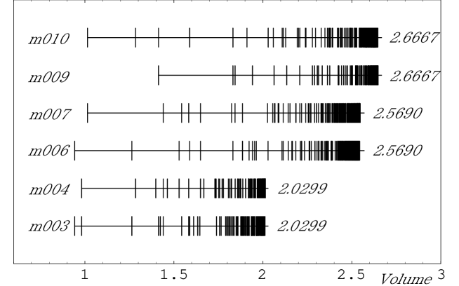
Figure 2.1: Volume Spectra of CH manifolds

A prefix “m” in the labeling number represents a cusped manifold obtained by gluing five or fewer ideal tetrahedra. The numbers in the right side denote the volumes of the corresponding cusped manifold. The volumes have been computed by using the SnapPea kernel.

As shown in figure 2.1, the volume spectra are discrete but there are many accumulation points which correspond to the volumes of various cusped manifolds. The smallest cusped manifolds in the known manifolds have volume $2.0299$ which are labeled as “m003” and “m004”in SnapPea. m003 and m004 are topologically equivalent to the complement of a certain knot in the lens space $L_{5,1}$ and the complement of a “figure eight knot” (figure 2.2), respectively[Matveev].

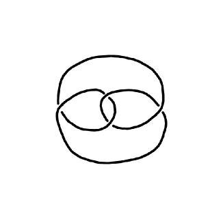
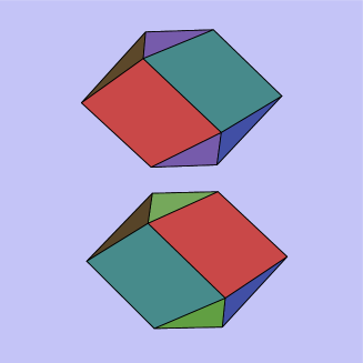
Figure 2.2: Cusped Hyperbolic Manifold

The figure in the left side represents a “figure eight knot” and the figure in the right shows the Dirichlet domain of a cusped manifold m004 viewed from two opposite directions in the Klein(projective) coordinates where geodesics and planes are mapped into their Euclidean counterparts. The two vertices on the left and right edges of the polyhedron which are identified by an element of the discrete isometry group correspond to a cusped point. Colors on the faces correspond to the identification maps. One obtains the Dirichlet domain of m003 by interchanging colors on quadrilateral faces in the lower(or upper) right figure.

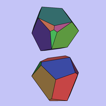
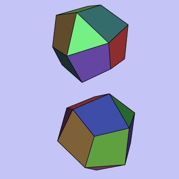
Figure 2.3: Smallest CH Manifolds

Dirichlet domains of the Weeks manifold (left) and the Thurston manifold(right) viewed from opposite directions in the Klein(projective) coordinates. Colors on the faces correspond to the identification maps. The manifolds can be obtained by performing (3,-1) and (-2,3) Dehn surgeries on m003, respectively.

(3,-1) and (-2, 3) Dehn surgeries on m003 yield the smallest and the second smallest known manifolds, which are called the Weeks manifold (volume=0.9427) and the Thurston manifold (volume=0.9814), respectively. It should be noted that the volume of CH manifolds must be larger than 0.16668… times cube of the curvature radius although no concrete examples of manifolds with such small volumes are known[GMT96]. As $|p|$ and $|q|$ becomes large, the volumes converge to that of $M_{c}$. Similarly, one can do Dehn surgeries on m004 or other cusped manifolds to obtain a different series of CH manifolds.

Chapter 3 Mode Functions

Science grows slowly and gently; reaching the truth by a variety of errors. One must prepare the introduction of a new idea through long and diligent labour; then, at a given moment, it emerges as if compelled by a divine necessity …

(Karl Gustav Jacob Jacobi, 1804-1851)

In locally isotropic and homogeneous background spaces each type (scalar, vector and tensor) of first-order perturbations can be decomposed into a decoupled set of equations. In order to solve the decomposed linearly perturbed Einstein equations, it is useful to expand the perturbations in terms of eigenmodes ($\!=\!$ eigenfunctions that are square-integrable) of the Laplace-Beltrami operator which satisfies the Helmholtz equation with certain boundary conditions

$$(\nabla^{2}+k^{2})u_{k}(x)=0,$$ (3.1)

since each eigenmode evolves independently. Then one can easily see that the time evolution of the perturbations in multiply-connected locally isotropic and homogeneous spaces coincide with those in the locally and globally homogeneous and isotropic FRWL spaces whereas the global structure of the background space is determined by these eigenmodes. In the simplest closed flat toroidal spaces obtained by gluing the opposite faces of a cube by three translations, the mode functions are given by plane waves with discrete wave numbers. In general, the mode functions in locally isotropic and homogeneous spaces can be written as a linear combination of eigenfunctions on the universal covering space.
The property of eigenmodes of CH spaces have not been unveiled until recently although a number of theorems concerning with lower bounds and upper bounds of eigenvalues in terms of diffeomorphism-invariant quantitities have been known in mathematical literature. However, despite the lack of knowledge about the property, eigenmodes of CH spaces have been numerically investigated by a number of authors in the field of number theory and harmonic analysis and of quantum chaology which are connected each other at a deep level. For the last 15 years, various numerical techniques have been applied to the eigenvalue problems for solving the Helmholtz equation (3.1) with periodic boundary conditions (manifold case), Neumann and Dirichlet boundary conditions (orbifold case). Eigenvalues of CH 2-spaces has been numerically obtained by many authors[Balazs, AS1, AS2, BSS, AS4, Hejhal]. Eigenvalues of cusped arithmetic and cusped non-arithmetic 3-manifolds with finite volume have been obtained by Grunewald and Huntebrinker using a finite element method[Grunewald]. Aurich and Marklof have computed eigenvalues of a non-arithmetic 3-orbifold using the direct boundary element method(DBEM)[AM]. The author has succeeded in computing low-lying eigenmodes of the Thurston manifold, the second smallest one using the DBEM[Inoue1], and later the Weeks manifold, the smallest one in the known CH manifolds using the same method[Inoue3]. Cornish and Spergel have also succeeded in calculating eigenmodes of these manifolds and 10 other CH manifolds based on the Trefftz method[CS99].
In quantum mechanics, an eigenmode can be interpreted as a wave function of a free particle at a stationary state with energy $E\!=\!k^{2}$. The statistical property of the energy eigenvalues $E$ and the eigenmodes $u_{E}$ of the classically chaotic systems has been investigated for exploring the imprints of classical chaos in the corresponding quantum system (e.g. see[Boh] and other articles therein). Because any classical dynamical systems of a free particle in CH spaces (known as the Hadamard-Gutzwiller models) are strongly chaotic (or more precisely they are K-systems with ergodicity, mixing and Bernoulli properties [Balazs]), it is natural to expect a high degree of complexity for each eigenstate. In fact, in many classically chaotic systems, it has been found that the short-range correlations observed in the energy states agree with the universal prediction of random matrix theory (RMT) for three universality classes:the Gaussian orthogonal ensemble(GOE), the Gaussian unitary ensemble(GUE) and the Gaussian symplectic ensemble (GSE)[Meh, Boh]. For the Hadamard-Gutzwiller models the statistical property of the eigenvalues and eigenmodes is described by GOE (which consist of real symmetric $N\!\times\!N$ matrices $H$ which obey the Gaussian distribution $\propto\exp{(-\textrm{Tr}H^{2}/(4a^{2}))}$ (where $a$ is a constant) as the systems possess a time-reversal symmetry. RMT also predicts that the squared expansion coefficients of an eigenstate with respect to a generic basis are distributed as Gaussian random numbers [Brody] which had been numerically confirmed for some classically chaotic systems ([AS4, Haake]). Although these results are for highly excited modes in the semiclassical region, low-lying modes may also retain the random property. For the analysis of CMB temperature fluctuations, the statistical property of the expansion coefficients of low-lying eigenmodes is of crucial importance since it is relevant to the ensemble averaged temperature correlations on the present horizon scales.
For classically chaotic systems, the semiclassical correspondence is given by the Gutzwiller trace formula[Gutzwiller] which relates a set of periodic orbits in the phase space to a set of energy eigenstates. Note that the correspondence is no longer one-to-one as in classically integrable systems. Interestingly, for CH spaces, the Gutzwiller trace formula gives an exact relation which had been known as the Selberg trace formula in mathematical literature[Selberg]. The trace formula gives an alternative method to compute the eigenvalues and eigenmodes in terms of periodic orbits. The poles of energy Green’s function are generated as a result of interference of waves each one of which corresponds to a periodic orbit. Roughly speaking, periodic orbits with shorter length contribute to the deviation from the asymptotic eigenvalue distribution on larger energy scales. In fact, a set of zero-length orbits produce Weyl’s asymptotic formula. Because periodic orbits can be obtained algebraically, the periodic orbit sum method enables one to compute low-lying eigenvalues for a large sample of manifolds or orbifolds systematically if each fundamental group is known beforehand. The method has been used to obtain eigenvalues of the Laplace-Beltrami operator on CH 2-spaces and a non-arithmetic 3-orbifold[AS1, AS3, AM]. However, it has not been applied to any CH 3-manifolds so far.
In section 1, we first formulate the DBEM for computing eigenmodes of the Laplace-Beltrami operator of CH 3-manifolds. In section 2, we study the statistical property of low-lying eigenmodes on the Weeks and the Thurston maniolds, which are the smallest examples in the known CH 3-manifolds. In section 3, we describe the method for computing the length spectra and derive an explicit form for computing the spectral staircase in terms of length spectrum which is applied for CH manifolds with volume less than 3. In section 4, we analyze the relation between the low- lying eigenvalues and several diffeomorphism-invariant geometric quantities, namely, volume, diameter and length of the shortest periodic geodesics. In the last section, the deviation of low-lying eigenvalue spectrum from the asymptotic distribution is measured by $\zeta-$ function and the spectral distance.

3.1 Boundary element method

3.1.1 Formulation

The boundary element methods (BEM) use a free Green’s function as the weighted function, and the Helmholtz equation is rewritten as an integral equation defined on the boundary using Green’s theorem. Discretization of the boundary integral equation yields a system of linear equations. Since one needs the discretization on only the boundary, BEM reduces the dimensionality of the problem by one, which leads to economy in the numerical task. To locate an eigenvalue, the DBEM requires one to compute many determinants of the corresponding boundary matrices which are dependent on the wavenumber $k$.
First, let us consider the Helmholtz equation with certain boundary conditions,

$$(\nabla^{2}+k^{2})u({\mathbf{x}})=0,$$ (3.2)

which is defined on a bounded M-dimensional connected and simply-connected domain $\Omega$ which is a subspace of a M-dimensional Riemannian manifold ${\cal M}$ and the boundary $\partial\Omega$ is piecewise smooth. $\nabla^{2}\equiv\nabla^{i}\nabla_{i},~{}(i=1,2,\cdot\cdot\cdot,M)$, and $\nabla_{i}$ is the covariant derivative operator defined on $\cal M$. A function $u$ in Sobolev space $H^{2}(\Omega)$ is the solution of the Helmholtz equation if and only if

$${\cal R}[u({\mathbf{x}}),v({\mathbf{x}})]\equiv\Bigl{\langle}(\nabla^{2}+k^{2})\ u({\mathbf{x}}),v({\mathbf{x}})\Bigr{\rangle}=0,$$ (3.3)

where $v$ is an arbitrary function in Sobolev space $H^{1}(\Omega)$ called weighted function and $\langle\,\rangle$ is defined as

$$\langle a,b\rangle\equiv\int_{\Omega}ab\sqrt{g}\,dV.$$ (3.4)

Next, we put $u({\mathbf{x}})$ into the form

$$u=\sum_{j=1}^{M}u_{j}\phi_{j},$$ (3.5)

where $\phi_{j}$’s are linearly independent square-integrable functions. Numerical methods such as the finite element methods try to minimize the residue function $\cal R$ for a fixed weighted function $v({\mathbf{x}})$ by changing the coefficients $u_{j}$. In these methods, one must resort to the variational principle to find the $u_{j}$’s which minimize ${\cal R}$.
Now, we formulate the DBEM which is a version of BEMs. Here we search $u({\mathbf{x}})$’s for the space $C^{1}(\bar{\Omega})\cap C^{2}(\Omega)\cap L^{2}(\Omega)$. First, we slightly modify Eq.(3.3) using the Green’s theorem

$$\int_{\Omega}(\nabla^{2}u)v\sqrt{g}dV-\int_{\Omega}(\nabla^{2}v)u\sqrt{g}dV=\int_{\partial\Omega}(\nabla_{i}u)v\sqrt{g}dS^{i}-\int_{\partial\Omega}(\nabla_{i}v)u\sqrt{g}dS^{i},$$ (3.6)

where $g\equiv\mathrm{det}\{g_{ij}\}$ and $dV\equiv dx_{1}\ldots dx_{M}$; the surface element $dS^{i}$ is given by

$$dS_{i} \equiv \frac{1}{M!}\epsilon_{ij_{1}\cdot\cdot\cdot j_{M}}dS^{j_{1}\cdot\cdot\cdot j_{M}},$$

$$dS^{j_{1}\ldots j_{M}} \equiv \left|\begin{array}[]{@{\,}cccc@{\,}}dx^{(1)j_{1}}&dx^{(2)j_{1}}&\ldots&dx^{(M)j_{1}}\\ dx^{(1)j_{2}}&dx^{(2)j_{2}}&\ldots&dx^{(M)j_{2}}\\ \vdots&\vdots&\ddots&\vdots\\ dx^{(1)j_{M}}&dx^{(2)j_{M}}&\ldots&dx^{(M)j_{M}}\end{array}\right|,$$ (3.11)

where $\epsilon_{j_{1}\cdot\cdot\cdot j_{M+1}}$ denotes the M$\!+1$-dimensional Levi-Civita tensor. Then Eq.(3.3) becomes

$$\int_{\Omega}(\nabla^{2}v+k^{2}v)u\sqrt{g}\,dV+\int_{\partial\Omega}(\nabla_{i}u)v\sqrt{g}\,dS^{i}-\int_{\partial\Omega}(\nabla_{i}v)u\sqrt{g}\,dS^{i}=0.$$ (3.12)

As the weighted function $v$, we choose the fundamental solution $G_{E}({\mathbf{x}},{\mathbf{y}})$ which satisfies

$$(\nabla^{2}+E)G_{E}({\mathbf{x}},{\mathbf{y}})=\delta_{D}({\mathbf{x}}-{\mathbf{y}}),$$ (3.13)

where $E\equiv k^{2}$, and $\delta_{D}({\mathbf{x}}-{\mathbf{y}})$ is Dirac’s delta function. $G_{E}({\mathbf{x}},{\mathbf{y}})$ is also known as the free Green’s function whose boundary condition is given by

$$\lim_{d({\mathbf{x}},{\mathbf{y}})\rightarrow\infty}G_{E}({\mathbf{x}},{\mathbf{y}})=0,$$ (3.14)

where $d({\mathbf{x}},{\mathbf{y}})$ is the geodesic distance between ${\mathbf{x}}$ and ${\mathbf{y}}$. Let ${\mathbf{y}}$ be an internal point of $\Omega$. Then we obtain from Eq.(3.12) and Eq.(3.13),

$$u({\mathbf{y}})+\int_{\partial\Omega}G_{E}({\mathbf{x}},{\mathbf{y}})\nabla_{i}u\,\sqrt{g}\,dS^{i}-\int_{\partial\Omega}(\nabla_{i}G_{E}({\mathbf{x}},{\mathbf{y}}))u\,\sqrt{g}\,dS^{i}=0.$$ (3.15)

Thus the values of eigenfunctions at internal points can be computed using only the boundary integral. If ${\mathbf{y}}\in\partial\Omega$, we have to evaluate the limit of the boundary integral terms as $G_{E}({\mathbf{x}},{\mathbf{y}})$ becomes divergent at ${\mathbf{x}}={\mathbf{y}}$ (see appendix A). The boundary integral equation is finally written as

$$\frac{1}{2}u({\mathbf{y}})+\int_{\partial\Omega}G_{E}({\mathbf{x}},{\mathbf{y}})\nabla_{i}u\,\sqrt{g}\,dS^{i}-\int_{\partial\Omega}(\nabla_{i}G_{E}({\mathbf{x}},{\mathbf{y}}))u\,\sqrt{g}\,dS^{i}=0,$$ (3.16)

or in another form,

$$\frac{1}{2}u({\mathbf{y}})+\int_{\partial\Omega}G_{E}({\mathbf{x}},{\mathbf{y}})\frac{\partial u}{\partial x^{i}}n^{i}\,\sqrt{g}\,dS-\int_{\partial\Omega}\frac{\partial G_{E}({\mathbf{x}},{\mathbf{y}})}{\partial x^{i}}n^{i}\,u\,\sqrt{g}\,dS=0,$$ (3.17)

where $n^{i}\equiv dS^{i}/dS$ and $dS\equiv\sqrt{dS^{i}\,dS_{i}}$. Note that we assumed that the boundary surface at ${\mathbf{y}}$ is sufficiently smooth. If the boundary is not smooth, one must calculate the internal solid angle at ${\mathbf{y}}$ (see appendix A). Another approach is to rewrite Eq.(3.15) in a regularized form [Tan]. We see from Eq.(3.16) or Eq.(3.17) that the approximated solutions can be obtained without resorting to the variational principle. Since it is virtually impossible to solve Eq.(3.17) analytically, we discretize it using boundary elements. Let the number of the elements be N. We approximate $u$ by some low-order polynomials (shape function) on each element as $u=c_{1}+c_{2}\,\eta+c_{3}\,\xi$ where $\eta$ and $\xi$ denote the coordinates on the corresponding standard element .

Then we have the following equation:

$$[H]\{u\}=[G]\{q\},~{}~{}~{}~{}q\equiv\frac{\partial u}{\partial n},$$ (3.18)

where {u} and {q} are $N$-dimensional vectors which consist of the boundary values of an eigenfunction and its normal derivatives, respectively. [H] and [G] are $N\times N$-dimensional coefficient matrices which are obtained from integration of the fundamental solution $G_{E}({\mathbf{x}},{\mathbf{y}})$ and its normal derivatives multiplied by $u_{i}$ and $q_{i}$, respectively. Note that the elements in [H] and [G] include $k$ implicitly. Because Eq.(3.18) includes both $u$ and $q$, the boundary element method can naturally incorporate the periodic boundary conditions:

$$u({\mathbf{x}})=u(g_{i}({\mathbf{x}})),~{}~{}~{}q({\mathbf{x}})=-q(g_{i}({\mathbf{x}})),~{}~{}\textrm{on}~{}~{}\partial\Omega,$$ (3.19)

where $g_{i}$’s are the face-to-face identification maps defined on the boundary. The boundary conditions constrain the number of unknown constants to $N$. Application of the boundary condition (3.19) to Eq.(3.18) and permutation of the columns of the components yields

$$[A]\{x\}=0,$$ (3.20)

where $N\times N$-dimensional matrix $A$ is constructed from $G_{ij}$ and $H_{ij}$ and $N$-dimensional vector $x$ is constructed from $u_{i}$’s and $q_{i}$’s. For the presence of the non-trivial solution, the following relation must hold,

$$\mathrm{det}[A]=0.$$ (3.21)

Thus, the eigenvalues of the Laplace-Beltrami operator acting on the space $C^{1}(\bar{\Omega})\cap C^{2}(\Omega)\cap L^{2}(\Omega)$ are obtained by searching for $k$’s which satisfy Eq.(3.21).

3.1.2 Computation of low-lying eigenmodes

In this section, we apply the DBEM for computing the low-lying eigenmodes of CH 3-manifolds. The Helmholtz equation in the Poincar$\acute{\textrm{e}}$ coordinates is written as

$$\frac{1}{4}\biggl{(}1-|{\mathbf{x}}|^{2}\biggr{)}^{2}\Biggl{[}\Delta_{E}+\frac{2}{1-|{\mathbf{x}}|^{2}}~{}~{}{\mathbf{x}}\cdot\nabla_{E}\Biggr{]}u+k^{2}u=0,$$ (3.22)

where $\Delta_{E}$ and $\nabla_{E}$ are the Laplacian and the gradient on the corresponding three-dimensional Euclidean space, respectively. Note that we have set the curvature radius $R=1$ without loss of generality. By using the DBEM, the Helmholtz equation (3.22) is converted to an integral representation on the boundary. Here Eq.(3.17) can be written in terms of Euclidean quantities as

$$\frac{1}{2}u({\mathbf{y}})+\int_{\partial\Omega}G_{k}({\mathbf{x}},{\mathbf{y}})\frac{\partial u}{\partial x^{i}}\,n_{E}^{i}\,dS-\int_{\partial\Omega}\frac{\partial G_{k}({\mathbf{x}},{\mathbf{y}})}{\partial x^{i}}\,u\,n_{E}^{i}\,dS=0,$$ (3.23)

where $dS=2(1-|{\mathbf{x}}|^{2})^{-1}\,dS_{E}$. The fundamental solution is given as [Els, Tom]

$$G_{k}\,({\mathbf{x}},{\mathbf{y}})=-\frac{1}{4\pi}\,\,\frac{\Bigl{(}\sigma+\sqrt{\sigma^{2}-1}\Bigr{)}^{-s}}{\sqrt{\sigma^{2}-1}},~{}~{}~{}-\frac{\pi}{2}<\mathrm{arg}\,\,s\leq\frac{\pi}{2},$$ (3.24)

where $s=\sqrt{1-k^{2}}$ and  $\sigma=\cosh d({\mathbf{x}},{\mathbf{y}})$. Then Eq.(3.23) is discretized on the boundary elements $\Gamma_{J}$ as

$$\frac{1}{2}u({\mathbf{x}}_{I})+\sum_{J=1}^{N}\Biggl{[}\int_{\Gamma_{J}}G_{k}({\mathbf{x}}_{I},{\mathbf{y}}_{J})\frac{\partial u({\mathbf{y}}_{J})}{\partial n}\,dS-\int_{\Gamma_{J}}\frac{\partial G_{k}({\mathbf{x}}_{I},{\mathbf{y}}_{J})}{\partial n}u({\mathbf{y}}_{J})\,dS\Biggr{]}=0,$$ (3.25)

where $N$ denotes the number of the boundary elements. An example of $N\!=\!1168$ elements on the boundary of the fundamental domain in the Poincar$\acute{\textrm{e}}$ coordinates is shown in figure 3.1. These elements are firstly generated in Klein coordinates in which the mesh-generation is convenient.

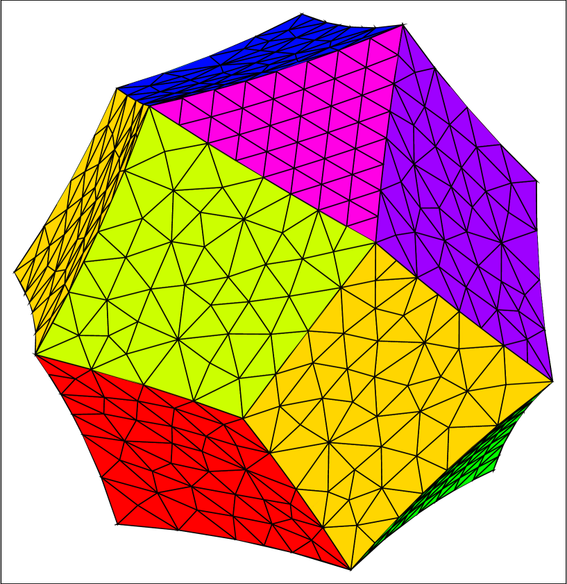
Figure 3.1: 1168 Boundary Elements

The maximum length of the edge $\Delta l$ in these elements is 0.14. The condition that the corresponding de Broglie wavelength $2\pi/k$ is longer than the four times of the interval of the boundary elements yields a rough estimate of the validity condition of the calculation as $k\!<\!11$. On each $\Gamma_{J}$, u and q $\equiv\partial u/\partial n$ are approximated by low order polynomials. For simplicity, we use constant elements:

$$u({\mathbf{x}}_{J})=u^{J}=Const.\,,~{}~{}~{}~{}q({\mathbf{x}}_{J})=q^{J}=Const.\,,~{}~{}~{}\mathrm{on}~{}~{}\Gamma_{J}.$$ (3.26)

Substituting Eq.(3.26) into Eq.(3.25), we obtain

$$\sum_{J=1}^{N}H_{IJ}u^{J} = \sum_{J=1}^{N}G_{IJ}q^{J},$$

$$H_{IJ} = \left\{\begin{array}[]{@{\,}ll}\tilde{H}_{IJ}&\mbox{$I\neq J$}\\ \tilde{H}_{IJ}-\frac{1}{2}&\mbox{$I=J$},\end{array}\right.$$

where

$$\tilde{H}_{IJ}\equiv\int_{\Gamma_{J}}\frac{\partial G_{k}}{\partial n}({\mathbf{x}}_{I},{\mathbf{y}}_{J})\,dS({\mathbf{y}}_{J}),~{}~{}G_{IJ}\equiv\int_{\Gamma_{J}}G_{k}({\mathbf{x}}_{I},{\mathbf{y}}_{J})\,dS({\mathbf{y}}_{J}).$$ (3.29)

The singular integration must be carried out for I-I components as the fundamental solution diverges at (${\mathbf{x}}_{I}={\mathbf{y}}_{I}$). This is not an intractable problem. Several numerical techniques have already been proposed by some authors [Tel, Hay]. We have applied Hayami’s method to the evaluation of the singular integrals [Hay]. Introducing coordinates similar to spherical coordinates centered at ${\mathbf{x}}_{I}$, the singularity is canceled out by the Jacobian which makes the integral regular.
Let $g_{i}\,{(i\!=\!1,2,\ldots,8)}$ be the generators of the discrete group $\Gamma$ which identify a boundary face $F_{i}$ with another boundary face $g_{i}(F_{i})$:

$$g_{i}({\mathbf{x}}_{i})={\mathbf{x}}_{i},~{}~{}~{}~{}~{}~{}~{}~{}~{}~{}~{}{\mathbf{x}}_{i}\in F_{i}.$$ (3.30)

The boundary of the fundamental domain can be divided into two regions $\partial\Omega_{A}$ and $\partial\Omega_{B}$ and each of them consists of $N/2$ boundary elements,

$$\partial\Omega_{A}={\cup F_{i}},~{}~{}~{}~{}~{}~{}~{}~{}\partial\Omega_{B}={\cup g_{i}(F_{i})},~{}~{}i=1,2,\ldots,8.$$ (3.31)

The periodic boundary conditions

$$u(g_{i}({\mathbf{x}}_{i}))=u({\mathbf{x}}_{i}),~{}~{}~{}~{}q(g_{i}({\mathbf{x}}_{i}))=-q({\mathbf{x}}_{i}),~{}~{}~{}~{}~{}~{}i=1,2,\ldots,8$$ (3.32)

reduce the number of the independent variables to N, i.e. for all ${\mathbf{x}}_{B}\in\partial\Omega_{B}$, there exist $g_{i}\in\Gamma$ and ${\mathbf{x}}_{A}\in\partial\Omega_{A}$ such that

$$u({\mathbf{x}}_{B})=u(g_{i}({\mathbf{x}}_{A}))=u({\mathbf{x}}_{A}),~{}~{}~{}~{}q({\mathbf{x}}_{B})=-q(g_{i}({\mathbf{x}}_{A}))=-q({\mathbf{x}}_{A}).$$ (3.33)

Substituting the above relation into Eq.(3.29), we obtain

$$\left[\begin{array}[]{@{\,}cc@{\,}}H_{AA}+H_{AB}&-G_{AA}+G_{AB}\\ H_{BA}+H_{BB}&-G_{BA}+G_{BB}\end{array}\right]\left\{\begin{array}[]{@{\,}c@{\,}}u_{A}\\ q_{A}\end{array}\right\}=0,$$ (3.34)

where $u_{A}=(u^{1},u^{2},\ldots u^{N/2})$ and $q_{A}=(q^{1},q^{2},\ldots q^{N/2})$ and matrices $H=\{H_{IJ}\}$ and $G=\{G_{IJ}\}$ are written as

$$H=\left[\begin{array}[]{@{\,}cc@{\,}}H_{AA}&H_{AB}\\ H_{BA}&H_{BB}\end{array}\right],~{}~{}~{}G=\left[\begin{array}[]{@{\,}cc@{\,}}G_{AA}&G_{AB}\\ G_{BA}&G_{BB}\end{array}\right].$$ (3.35)

Eq. (3.34) takes the form

$$[A(k)]\{x\}=0,$$ (3.36)

where $N\times N$-dimensional matrix $A$ is constructed from $G$ and $H$ and $N$-dimensional vector $x$ is constructed from $u_{A}$ and $q_{A}$. For the presence of the non-trivial solution, the following relation must hold,

$$\mathrm{det}[A(k)]=0.$$ (3.37)

Thus the eigenvalues of the Laplace-Beltrami operator in a CH space are obtained by searching for $k$’s which satisfy Eq.(3.37). In practice, Eq.(3.37) cannot be exactly satisfied as the test function which has a locally polynomial behavior is slightly deviated from the exact eigenfunction. Instead, one must search for the local minima of det[A(k)]. This process needs long computation time as $A(k)$ depends on k implicitly. Our numerical result ($k\!<\!13$) is shown in table 3.1.

Weeks				Thurston
$k$	$m(k)$	$k$	$m(k)$	$k$	$m(k)$	$k$	$m(k)$
5.268	1	11.283	1	5.404	1	10.686	2
5.737	2	11.515	1	5.783	1	10.737	1
6.563	1	11.726	4	6.807	2	10.830	1
7.717	1	12.031	2	6.880	1	11.103	2
8.162	1	12.222	2	7.118	1	11.402	1
8.207	2	12.648	1	7.686	2	11.710	1
8.335	2	12.789	1	8.294	1	11.728	1
9.187	1			8.591	1	11.824	1
9.514	1			8.726	1	12.012	2
9.687	1			9.246	1	12.230	1
9.881	2			9.262	1	12.500	1
10.335	2			9.754	1	12.654	1
10.452	2			9.904	1	12.795	1
10.804	1			9.984	1	12.806	1
10.857	1			10.358	1	12.897	2

Table 3.1: Eigenvalue k and Multiplicity $m(k)$

The first ”excited state” that corresponds to $k\!=\!k_{1}$ is important for the understanding of CMB anisotropy. Our numerical result $k_{1}\!=\!5.41$ is consistent with the value $5.04$ obtained from Weyl’s asymptotic formula

$$N[\nu]=\frac{V\!o\,l({\cal M})\nu^{3}}{6\pi^{2}},~{}~{}\nu\equiv\sqrt{k^{2}-1},~{}~{}~{}~{}\nu\!>\!>\!1,$$ (3.38)

assuming that no degeneracy occurs. One can interpret the first excited state as the mode that has the maximum de Broglie wavelength $2\pi/k_{1}$. Because of the periodic boundary conditions, the de Broglie wavelength can be approximated by the ”average diameter” of the fundamental domain defined as a sum of the inradius $r_{-}$ and the outradius $r_{+}$, which yields $k_{1}=4.9$ just $10\!\%$ less than the numerical value. From these estimates, supercurvature modes in small CH spaces ($Vol({\cal M})\sim 1$) are unlikely to be observed.
To compute the value of eigenfunctions inside the fundamental domain, one needs to solve Eq.(3.36). The singular decomposition method is the most suitable numerical method for solving any linear equation with a singular matrix $A$, which can be decomposed as

$$A=U^{\dagger}DV,$$ (3.39)

where $U$ and $V$ are unitary matrices and D is a diagonal matrix. If $D_{ii}$ in $D$ is almost zero then the complex conjugate of the i-th row in V is an approximated solution of Eq.(3.36). The number of the ”almost zero” diagonal elements in D is equal to the multiplicity number.

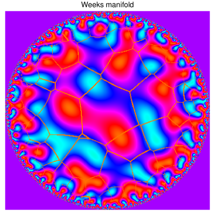
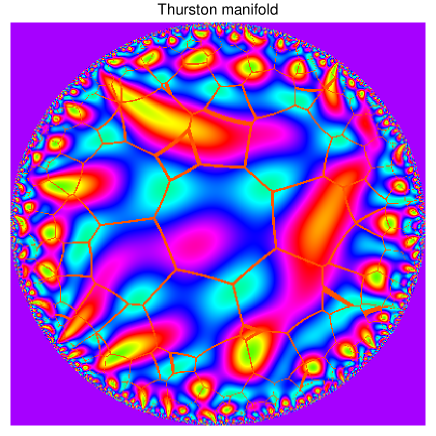
Figure 3.2: Lowest Eigenmodes

The lowest eigenmodes of the Weeks manifold $(k\!=\!5.268)$ and the Thurston manifold $(k\!=\!5.404)$ on a slice $z\!=\!0$ in the Poincar$\acute{\textrm{e}}$ coordinates. The boundaries of the copied Dirichlet domains (solid curves) are plotted in full curve.

Substituting the values of the eigenfunctions and their normal derivatives on the boundary into Eq.(3.15), the values of the eigenfunctions inside the fundamental domain can be computed. Adjusting the normalization factors, one would obtain real-valued eigenfunctions. Note that non-degenerated eigenfunctions must be always real-valued.
The numerical accuracy of the obtained eigenvalues is roughly estimated as follows. First, let us write the obtained numerical solution in terms of the exact solution as $k=k_{0}+\delta k$ and $u_{k}({\mathbf{x}})=u_{k_{0}}({\mathbf{x}})+\delta u_{k}({\mathbf{x}})$, where $k_{0}$ and $u_{k_{0}}({\mathbf{x}})$ are the exact eigenvalue and eigenfunction, respectively. The singular decomposition method enables us to find the best approximated solution which satisfies

$$[A]\{x\}=\epsilon,~{}~{}~{}|\epsilon|<<1,$$ (3.40)

where $\epsilon$ is a N-dimensional vector and $|~{}|$ denotes the Euclidean norm. It is expected that the better approximation gives the smaller $|\epsilon|$. Then Eq. (3.40) can be written as,

$$\int_{\Omega}G_{k_{0}+\delta k}({\mathbf{x}},{\mathbf{y}}_{J})(\Delta+(k_{0}+\delta k)^{2})(u_{k_{0}}({\mathbf{x}})+\delta u_{k}({\mathbf{x}}))\,\sqrt{g}\,dV_{\mathbf{x}}=\epsilon({\mathbf{y}}_{J}).$$ (3.41)

Ignoring the terms in second order, Eq.(3.41) is reduced to

$$\int_{\Omega}G_{k}({\mathbf{x}},{\mathbf{y}}_{J})((\Delta+k_{0}^{2})\delta u_{k}({\mathbf{x}})+2k\delta ku_{k}({\mathbf{x}}))\,\sqrt{g}\,dV_{\mathbf{x}}=\epsilon({\mathbf{y}}_{J}).$$ (3.42)

Since it is not unlikely that $(\Delta+k_{0}^{2})\delta u_{k}({\mathbf{x}})$ is anticorrelated to $2k\delta ku_{k}({\mathbf{x}})$, we obtain the following relation by averaging over ${\mathbf{y}}_{J}$,

$$2k|\delta k|\Biggl{<}\biggl{|}\int_{\Omega}G_{k}({\mathbf{x}},{\mathbf{y}}_{J})u_{k}({\mathbf{x}})\,\sqrt{g}\,dV_{\mathbf{x}}\biggr{|}\Biggr{>}\sim\,\,<|\epsilon|>,$$ (3.43)

where $<>$ denotes the averaging over ${\mathbf{y}}_{J}$ Thus one can estimate the expected deviation of the calculated eigenvalue $|\delta k|$ from $u_{k}({\mathbf{x}})$ and $\epsilon({\mathbf{y}}_{J})$. We numerically find that $|\delta k|=0.005$ for $k=5.41$ and $|\delta k|=0.01$ for $k=9.91$(Thurston manifolds). The other deviation values lie in between $0.005$ and $0.01$.
By computing the second derivatives, one can also estimate the accuracy of the computed eigenfunctions. The accuracy parameter $err$ is defined as

$$err(k,{\mathbf{x}})\equiv(\Delta+k^{2})u_{k}({\mathbf{x}}),$$ (3.44)

Figure 3.3: Error Estimation

Errors ($err$) in terms of hyperbolic distance $d$ to the boundary from 291 points in the fundamental domain of the Thurston manifold.

where $u_{k}({\mathbf{x}})$ is normalized (${\cal O}(u_{k}({\mathbf{x}}))\sim 1$). We see from figure 3.3 that the accuracy becomes worse as the evaluation point approaches the boundary. However, for points with hyperbolic distance $d>0.1$ between the evaluating point and the nearest boundary, the errors are very small indeed: $err=10^{-4\sim-5}$. This result is considered to be natural because the characteristic scale $L$ of the boundary elements is $\sim 0.07$ for our 1168 elements. If $d<L$, the integrands in Eq.(3.15) become appreciable on the neighborhood of the nearest boundary point because the free Green’s function approximately diverges on the point. In this case, the effect of the deviation from the exact eigenfunction is significant. If $d>>L$, the integrand on all the boundary points contributes almost equally to the integration so that the local deviations are cancelled out.
As we shall see in the next section, expansion coefficients are calculated using the values of eigenfunctions on a sphere. Since the number of evaluating points which are very close to the boundary is negligible on the sphere, expansion coefficients can be computed with relatively high accuracy.

3.1.3 Statistical property of eigenmodes

In pseudospherical coordinates ($R,\chi,\theta,\phi$), the eigenmodes are written in terms of complex expansion coefficients $\xi_{\nu lm}$ and eigenmodes on the universal covering space,

$$u_{\nu}=\sum_{lm}\xi_{\nu lm}\,X_{\nu l}(\chi)Y_{lm}(\theta,\phi),$$ (3.45)

where $\nu=\sqrt{k^{2}-1}$ and $Y_{lm}$ is a (complex) spherical harmonic. The radial eigenfunction $X_{\nu l}$ is written in terms of the associated Legendre function $P$, and the $\Gamma$ function as

$$X_{\nu l}=\frac{\Gamma(l+1+\nu i)}{\Gamma(\nu i)}\sqrt{\frac{1}{\sinh\chi}}P^{-l-1/2}_{\nu i-1/2}(\cosh\chi),~{}~{}~{}~{}\nu^{2}=k^{2}-1.$$ (3.46)

Then the real expansion coefficients $a_{\nu lm}$ are given by

$$a_{\nu 00} = -\textrm{Im}(\xi_{\nu 00}),~{}~{}~{}~{}a_{\nu l0}=\sqrt{c_{\nu l}}\textrm{Re}(\xi_{\nu l0}),$$

$$a_{\nu lm} = \sqrt{2}\textrm{Re}(\xi_{\nu lm}),~{}~{}m>0,$$

$$a_{\nu lm} = -\sqrt{2}\textrm{Im}(\xi_{\nu l-m}),~{}~{}m<0,$$ (3.47)

where

$$c_{\nu l} = \frac{2}{(1+\textrm{Re}(F(\nu,l)))},$$

$$F(\nu,l) = \frac{\Gamma(l+\nu i+1)}{\Gamma(\nu i)}\frac{\Gamma(-\nu i)}{\Gamma(l-\nu i+1)}.$$ (3.48)

$a_{\nu lm}$ ’s can be promptly obtained after the normalization and orthogonalization of these eigenmodes. The orthogonalization is achieved at the level of $10^{-3}$ to $10^{-4}$ (for the inner product of the normalized eigenmodes) which implies that each eigenmode is computed with relatively high accuracy.

Figure 3.4: Random Nature of Expansion Coefficients

Expansion coefficients $a_{\nu lm}$ are plotted in ascending order as $l(l+1)+m+1,0\leq l\leq 20$ for eigenmodes $k\!=\!5.268$(left) and $k\!=\!12.789$(right) on the Weeks manifold at a point which is randomly chosen.

In figure 3.4 one can see that the distribution of $a_{\nu lm}$’s, which are ordered as $l(l+1)+m+1$ are qualitatively random. In order to estimate the randomness quantitatively, we consider a cumulative distribution of

$$b_{\nu lm}=\frac{|a_{\nu lm}-\bar{a}_{\nu}|^{2}}{\sigma_{\nu}^{2}}$$ (3.49)

where $\bar{a}_{\nu}$ is the mean of $a_{\nu lm}$’s and $\sigma_{\nu}^{2}$ is the variance. If $a_{\nu lm}$’s are Gaussian then $b_{\nu lm}$ ’s obey a $\chi^{2}$ distribution $P(x)=(1/2)^{1/2}\Gamma(1/2)x^{-1/2}e^{-x/2}$ with 1 degree of freedom. To test the goodness of fit between the the theoretical cumulative distribution $I(x)$ and the empirical cumulative distribution function $I_{N}(x)$, we use the Kolmogorov-Smirnov statistic $D_{N}$ which is defined as the least upper bound of all pointwise differences $|I_{N}(x)-I(x)|$ [Hog],

$$D_{N}\equiv\sup_{x}|I_{N}(x)-I(x)|,$$ (3.50)

where $I_{N}(x)$ is defined as

$$I_{N}(x) = \left\{\begin{array}[]{@{\,}ll}0,&x<y_{1},\\ j/N,{}{}&y_{j}\leq x<y_{j+1},~{}~{}~{}~{}j=1,2,\ldots,N\!-\!1,\\ 1,&y_{N}\leq x,\end{array}\right.$$ (3.54)

and $y_{1}<y_{2}<\ldots<y_{N}$ are the computed values of a random sample which consists of $N$ elements. For random variables $D_{N}$ for any $z>0$, it can be shown that the probability of $D_{N}\!<\!d$ is given by [Bir]

$$\lim_{N\rightarrow\infty}~{}P(D_{N}<d=zN^{-1/2})=L(z),$$ (3.55)

where

$$L(z)=1-2\sum_{j=1}^{\infty}(-1)^{j-1}e^{-2j^{2}z^{2}}.$$ (3.56)

From the observed maximum difference $D_{N}\!=\!d$, we obtain the significance level $\alpha_{D}\!=\!1-P$, which is equal to the probability of $D_{N}\!>\!d$. If $\alpha_{D}$ is found to be large enough, the hypothesis $I_{N}(x)\!\neq\!I(x)$ is not verified. The significance levels $\alpha_{D}$ for $0\!\leq\!l\!\leq\!20$ and for eigenmodes $k\!<\!13$ on the Thurston manifold are shown in table 3.2.

Thurston
k	$\alpha_{D}$	k	$\alpha_{D}$
5.404	0.98	10.686b	$7.9\times 10^{-4}$
5.783	0.68	10.737	0.96
6.807a	0.52	10.830	0.67
6.807b	$7.1\times 10^{-4}$	11.103a	0.041
6.880	1.00	11.103b	$8.8\times 10^{-15}$
7.118	0.79	11.402	0.98
7.686a	0.26	11.710	0.92
7.686b	$2.3\times 10^{-8}$	11.728	0.93
8.294	0.45	11.824	0.31
8.591	0.91	12.012a	0.52
8.726	1.00	12.012b	0.73
9.246	0.28	12.230	0.032
9.262	0.85	12.500	0.27
9.754	0.39	12.654	0.88
9.904	0.99	12.795	0.76
9.984	0.20	12.806	0.42
10.358	0.40	12.897a	0.87
10.686a	0.76	12.897b	$6.9\times 10^{-4}$

Table 3.2: Kolmogorov-Smirnov Test I

Eigenvalues $k$ and the corresponding significance levels $\alpha_{D}$ for the test of the hypothesis $I_{N}(x)\neq I(x)$ for the Thurston manifold are listed. The injectivity radius is maximal at the base point.

The agreement with the RMT prediction is fairly good for most of eigenmodes which is consistent with the previous computation in [Inoue1]. However, for five degenerated modes, the non-Gaussian signatures are prominent (in [Inoue1], two modes in ($k\!<\!10$) have been missed). Where does this non-Gaussianity come from?
First of all, we must pay attention to the fact that the expansion coefficients $a_{\nu lm}$ depend on the observing point. In mathematical literature, the point is called the base point. For a given base point, it is possible to construct a particular class of fundamental domain called the Dirichlet (fundamental) domain which is a convex polyhedron. A Dirichlet domain $\Omega(x)$ centered at a base point $x$ is defined as

$$\Omega(x)=\bigcap_{g}H(g,x)~{}~{}~{},H(g,x)=\{z|d(z,x)<d(g(z),x)\},$$ (3.57)

where $g$ is an element of a Kleinian group $\Gamma$(a discrete isometry group of $PSL(2,{\mathbb{C}})$) and $d(z,x)$ is the proper distance between $z$ and $x$.
The shape of the Dirichlet domain depends on the base point but the volume is invariant. Although the base point can be chosen arbitrarily, it is a standard to choose a point $Q$ where the injectivity radius is locally maximal. More intuitively, $Q$ is a center where one can put a largest connected ball on the manifold. If one chooses other point as the base point, the nearest copy of the base point can be much nearer. The reason to choose $Q$ as a base point is that one can expect the corresponding Dirichlet domain to have many symmetries at $Q$ [Weeks2].

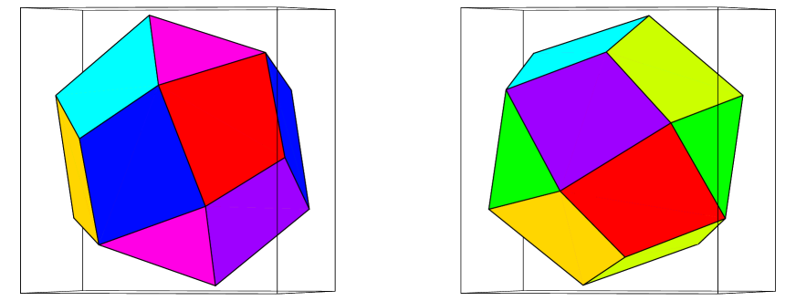
Figure 3.5: $Z^{2}$ Symmetry

A Dirichlet domain of the Thurston manifold in the Klein coordinates viewed from opposite directions at $Q$ where the injectivity radius is locally maximal. The Dirichlet domain has a $Z2$ symmetry(invariant by $\pi$-rotation)at $Q$.

As shown in figure 3.5 the Dirichlet domain at $Q$ has a $Z2$ symmetry (invariant by $\pi$-rotation) if all the congruent faces are identified. Generally, congruent faces are distinguished but it is found that these five modes have exactly the same values of eigenmodes on these congruent faces. Then one can no longer consider $a_{\nu lm}$’s as ”independent” random numbers. Choosing the invariant axis by the $\pi$-rotation as the $z$-axis, $a_{\nu lm}$’s are zero for odd $m$’s, leading to a non-Gaussian behavior. It should be noted that the observed $Z2$ symmetry is not the subgroup of the isometry group (or symmetry group in mathematical literature) $D2$ (dihedral group with order $2$) of the Thurston manifold since the congruent faces must be actually distinguished in the manifold.
Thus the observed non-Gaussianity is caused by a particular choice of the base point. However, in general, the chance that we actually observe any symmetries (elements of the isometry group of the manifold or the finite sheeted cover of the manifold) is expected to be very low. Because a fixed point by an element of the isometric group is either a part of 1-dimensional line (for instance, an axis of a rotation) or an isolated point (for instance, a center of an antipodal map).
In order to confirm that the chance is actually low, the KS statistics $\alpha_{D}$ of $a_{\nu lm}$’s are computed at 300 base points which are randomly chosen.

Weeks				Thurston
k	$<\alpha_{D}>$	k	$<\alpha_{D}>$	k	$<\alpha_{D}>$	k	$<\alpha_{D}>$
5.268	0.58	10.452b	0.62	5.404	0.63	10.686b	0.62
5.737a	0.61	10.804	0.63	5.783	0.61	10.737	0.62
5.737b	0.61	10.857	0.62	6.807a	0.62	10.830	0.63
6.563	0.62	11.283	0.57	6.807b	0.62	11.103a	0.59
7.717	0.59	11.515	0.61	6.880	0.63	11.103b	0.60
8.162	0.61	11.726a	0.63	7.118	0.61	11.402	0.61
8.207a	0.65	11.726b	0.59	7.686a	0.61	11.710	0.62
8.207b	0.61	11.726c	0.61	7.686b	0.63	11.728	0.64
8.335a	0.59	11.726d	0.61	8.294	0.60	11.824	0.62
8,335b	0.62	12.031a	0.60	8.591	0.60	12.012a	0.63
9.187	0.59	12.031b	0.60	8.726	0.60	12.012b	0.61
9.514	0.56	12.222a	0.61	9.246	0.60	12.230	0.60
9.687	0.61	12.222b	0.62	9.262	0.63	12.500	0.63
9.881a	0.61	12.648	0.59	9.754	0.62	12.654	0.62
9,881b	0.62	12.789	0.59	9.904	0.60	12.795	0.62
10.335a	0.63			9.984	0.60	12.806	0.62
10.335b	0.60			10.358	0.62	12.897a	0.62
10.452a	0.63			10.686a	0.60	12.897b	0.56

Table 3.3: Kolmogorov-Smirnov Test II

Eigenvalues $k$ and corresponding averaged significance levels $<\alpha_{D}>$ based on 300 realizations of the base points for the test of the hypothesis $I_{N}(x)\neq I(x)$ for the Weeks and the Thurston manifolds.

As shown in table (3.3), the averaged significance levels $<\!\alpha_{D}\!>$ are remarkably consistent with the Gaussian prediction. $1\sigma$ of $\alpha_{D}$ are found to be 0.26 to 0.30.
Next, we apply the run test for testing the randomness of $a_{\nu lm}$’s where each set of $a_{\nu lm}$ ’s are ordered as $l(l+1)+m+1$ (see [Hog]). Suppose that we have $n$ observations of the random variable $U$ which falls above the median and n observations of the random variable $L$ which falls below the median. The combination of those variables into $2n$ observations placed in ascending order of magnitude yields

UUU LL UU LLL U L UU LL,

Each underlined group which consists of successive values of $U$ or $L$ is called run. The total number of run is called the run number. The run test is useful because the run number always obeys the Gaussian statistics in the limit $n\!\rightarrow\!\infty$ regardless of the type of the distribution function of the random variables.

Weeks				Thurston
k	$<\alpha_{r}>$	k	$<\alpha_{r}>$	k	$<\alpha_{r}>$	k	$<\alpha_{r}>$
5.268	0.51	10.452b	0.52	5.404	0.48	10.686b	0.51
5.737a	0.48	10.804	0.52	5.783	0.45	10.737	0.49
5.737b	0.45	10.857	0.53	6.807a	0.53	10.830	0.53
6.563	0.54	11.283	0.49	6.807b	0.50	11.103a	0.52
7.717	0.50	11.515	0.51	6.880	0.47	11.103b	0.53
8.162	0.54	11.726a	0.51	7.118	0.50	11.402	0.51
8.207a	0.52	11.726b	0.48	7.686a	0.49	11.710	0.51
8.207b	0.49	11.726c	0.49	7.686b	0.52	11.728	0.49
8.335a	0.53	11.726d	0.48	8.294	0.50	11.824	0.54
8,335b	0.50	12.031a	0.54	8.591	0.50	12.012a	0.51
9.187	0.53	12.031b	0.51	8.726	0.51	12.012b	0.49
9.514	0.55	12.222a	0.54	9.246	0.43	12.230	0.51
9.687	0.53	12.222b	0.50	9.262	0.50	12.500	0.48
9.881a	0.51	12.648	0.54	9.754	0.54	12.654	0.48
9,881b	0.51	12.789	0.48	9.904	0.52	12.795	0.50
10.335a	0.54			9.984	0.49	12.806	0.51
10.335b	0.51			10.358	0.53	12.897a	0.57
10.452a	0.53			10.686a	0.51	12.897b	0.55

Table 3.4: Run Test

Eigenvalues $k$ and corresponding averaged significance levels $<\!\alpha_{r}\!>$ for the test of the hypothesis that the $a_{\nu lm}$’s are not random numbers for the Weeks and Thurston manifolds. $\alpha_{r}$’s at 300 points which are randomly chosen are used for the computation.

As shown in table 3.4, averaged significance levels $<\!\alpha_{r}\!>$ are very high (1$\sigma$ is 0.25 to 0.31). Thus each set of $a_{\nu lm}$’s ordered as $l(l+1)+m+1$ can be interpreted as a set of Gaussian pseudo-random numbers except for limited choices of the base point where one can observe symmetries of eigenmodes.
Up to now, we have considered $l$ and $m$ as the index numbers of $a_{\nu lm}$ at a fixed base point. However, for a fixed $(l,m)$, the statistical property of a set of $a_{\nu lm}$’s at a number of different base points is also important since the temperature fluctuations must be averaged all over the places for spatially inhomogeneous models. From figure 3.6, one can see the behavior of m-averaged significance levels

$$\alpha_{D}(\nu,l)\equiv\sum_{m=-l}^{l}\frac{\alpha_{D}(a_{\nu lm})}{2l+1}$$ (3.58)

which are calculated based on 300 realizations of the base points. It should be noted that each $a_{\nu lm}$ at a particular base point is now considered to be ”one realization” whereas a choice of $l$ and $m$ is considered to be ”one realization” in the previous analysis. The good agreement with the RMT prediction for components $l\!>\!1$ has been found. For components $l\!=\!1$, the disagreement occurs for only several modes. However, the non-Gaussian behavior is distinct in $l\!=\!0$ components. What is the reason of the non-Gaussian behavior for $l\!=\!0$?

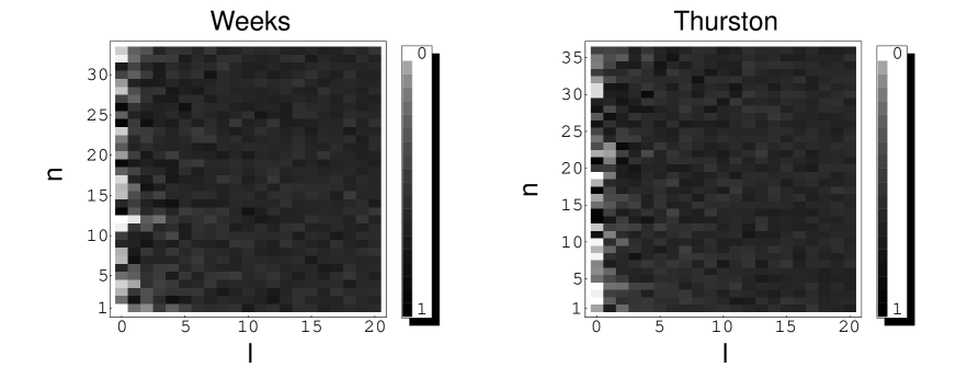
Figure 3.6: Kolomogorov-Smirnov Test III

Plots of $m$-averaged significance levels $\alpha_{D}(\nu,l)$ based on 300 realizations for the Weeks and the Thurston manifolds ($0\!\leq\!l\!\leq\!20$ and $k<13$). $n$ denotes the index number which corresponds to an eigenmode $u_{k}$ where the number of eigenmodes less than $k$ is equal to $n$ ($k(n\!=\!1)$ is the lowest non-zero eigenvalue). The accompanying palettes show the correspondence between the level of the grey and the value.

Let us estimate the values of the expansion coefficients for $l\!=\!0$. In general, the complex expansion coefficients $\xi_{\nu lm}$ can be written as,

$$\xi_{\nu lm}(\chi_{0})=\frac{1}{X_{\nu l}(\chi_{0})}\int u_{\nu}(\chi_{0},\theta,\phi)\,Y^{*}_{lm}(\theta,\phi)d\Omega.$$ (3.59)

For $l\!=\!0$, the equation becomes

$$\xi_{\nu 00}(\chi_{0})=-\frac{i}{2\sqrt{2}}\frac{\sinh{\chi_{0}}}{\sin{\nu\chi_{0}}}\int u_{\nu}(\chi_{0},\theta,\phi)\,d\Omega.$$ (3.60)

Taking the limit $\chi_{0}\rightarrow 0$, one obtains,

$$\xi_{\nu 00}=-\frac{2\pi u_{\nu}(0)i}{\nu}.$$ (3.61)

Thus $a_{\nu 00}$ can be written in terms of the value of the eigenmode at the base point. As shown in figure 3.2 the lowest eigenmodes have only one ”wave” on scale of the topological identification scale $L$ (which will be defined later on) inside a single Dirichlet domain which implies that the random behavior within the domain may be not present. Therefore, for low-lying eigenmodes, one would generally expect non-Gaussianity in a set of $a_{\nu 00}$ ’s. However, for high-lying eigenmodes, this may not be the case since these modes have a number of ”waves” on scale of $L$ and they may change their values locally in an almost random fashion.
The above argument cannot be applicable to $a_{\nu lm}$ ’s for $l\!\neq\!0$ where ${X_{\nu l}}$ approaches zero in the limit $\chi_{0}\!\rightarrow\!0$ while the integral term

$$\int u_{\nu}(\chi_{0},\theta,\phi)\,Y^{*}_{lm}(\theta,\phi)d\Omega$$ (3.62)

also goes to zero because of the symmetric property of the spherical harmonics. Therefore $a_{\nu lm}$ ’s cannot be written in terms of the local value of the eigenmode for $l\!\neq\!0$. For these modes, it is better to consider the opposite limit $\chi_{0}\rightarrow\infty$. It is numerically found that a sphere with a very large radius $\chi_{0}$ intersects each copy of the Dirichlet domain almost randomly (the pulled back surface into a single Dirichlet domain chaotically fills up the domain). Then the values of the eigenmodes on the sphere with a very large radius vary in an almost random fashion. For large $\chi_{0}$, we have

$$X_{\nu l}(\chi_{0})\!\propto\!e^{-2\chi_{0}+\phi(\nu,l)i},$$ (3.63)

where $\phi(\nu,l)$ describes the phase factor. Therefore, the order of the integrand in Eq. (3.59) is approximately $e^{-2\chi_{0}}$ since Eq. (3.59) does not depend on the choice of $\chi_{0}$. As the spherical harmonics do not have correlation with the eigenmode $u_{\nu}(\chi_{0},\theta,\phi)$, the integrand varies almost randomly for different choices of $(l,m)$ or base points. Thus, we conjecture that Gaussianity of $a_{\nu lm}$’s have their origins in the chaotic property of the sphere with large radius in CH spaces. The property may be related to the classical chaos in geodesic flows .
Let us now consider the average and variance of the expansion coefficients. As the eigenmodes have oscillatory features, it is natural to expect that the averages are equal to zero. In fact, the averages of $<\!a_{\nu lm}\!>$ ’s over $0\!\leq\!l\!\leq\!20$ and $-l\!\leq\!m\!\leq\!-l$ and 300 realizations of base points for each $\nu$-mode are numerically found to be $0.006\pm 0.04-0.02$(1$\sigma$) for the Weeks manifold, and $0.003\pm 0.04-0.02$(1$\sigma$) for the Thurston manifold. Let us next consider the $\nu$-dependence ($k$-dependence) of the variances $Var(a_{\nu lm})$. In order to crudely estimate the $\nu$-dependence, we need the angular size $\delta\theta$ of the characteristic length of the eigenmode $u_{\nu}$ at $\chi_{0}$[Inoue1]

$$\delta\theta^{2}\approx\frac{16\pi^{2}~{}V\!o\,l(M)}{k^{2}(\sinh(2(\chi_{o}+r_{ave}))-\sinh(2(\chi_{o}-r_{ave}))-4r_{ave})},$$ (3.64)

where $V\!o\,l(M)$ denotes the volume of a manifold $M$ and $r_{ave}$ is the averaged radius of the Dirichlet domain. There is an arbitrariness in the definition of $r_{ave}$. Here we define $r_{ave}$ as the radius of a sphere with volume equivalent to the volume of the manifold,

$$V\!o\,l(M)=\pi(\sinh(2r_{ave})-2r_{ave}),$$ (3.65)

which does not depend on the choice of a base point. Here we define the topological identification length $L$ as $L\!=\!2r_{ave}$. For the Weeks and the Thurston manifolds, $L\!=\!1.19$ and $L\!=\!1.20$ respectively. From Eq. (3.64), for large $\chi_{0}$, one can approximate $u_{\nu}(\chi_{o})\sim u_{\nu}^{\prime}(\chi^{\prime}_{o})$ by choosing an appropriate radius $\chi^{\prime}_{o}$ that satisfies $\nu^{-2}\exp(-2\chi_{o})=\nu^{\prime-2}\exp(-2\chi^{\prime}_{o})$. Averaging Eq. (3.59) over $l$’s and $m$’s or the base points, for large $\chi_{0}$, one obtains,

$$\bigl{<}|\xi_{\nu^{\prime}lm}|^{2}\bigr{>}\sim\frac{\exp(-2\chi_{o})}{\exp(-2\chi^{\prime}_{o})}\bigl{<}|\xi_{\nu lm}|^{2}\bigr{>},$$ (3.66)

which gives $\bigl{<}|\xi_{\nu lm}|^{2}\bigr{>}\sim\nu^{-2}$. Thus, the variance of $a_{\nu lm}$’s is proportional to $\nu^{-2}$. The numerical results for the two CH manifolds shown in figure 3.7 clearly support the $\nu^{-2}$ dependence of the variance.

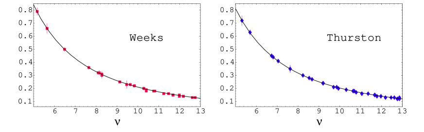
Figure 3.7: Variance of Expansion Coefficients

Averaged squared $a_{\nu}$’s ($k\!<\!13$) based on 300 realizations of the base points for the Weeks and the Thurston manifold with $\pm 1\sigma$ run-to-run variations. $a_{\nu}$ is defined to be $Var(a_{\nu lm})$ averaged over $0\!\leq\!l\!\leq\!20$ and $-l\!\leq\!m\!\leq\!l$. The best-fit curves for the Weeks and the Thurston manifolds are $21.0\nu^{-2}$ and $20.3\nu^{-2}$, respectively.

As we have seen, the property of eigenmodes on general CH manifolds is summarized in the following conjecture:

Conjecture: Except for the base points which are too close to any fixed points by symmetries, for a fixed $\nu$, a set of the expansion coefficients $a_{\nu lm}$ over $(l,m)$’s can be regarded as Gaussian pseudo-random numbers. For a fixed $(\nu lm)~{}(l>0)$, the expansion coefficients at different base points that are randomly chosen can be also regarded as Gaussian pseudo-random numbers. In either case, the variance is proportional to $\nu^{-2}$ and the average is zero.

3.2 Periodic orbit sum method

3.2.1 Length spectra

Computation of periodic orbits (geodesics) is of crucial importance for the semiclassical quantization of classically chaotic systems. However, in general, solving a large number of periodic orbits often becomes an intractable problem since the number of periodic orbits grows exponentially with an increase in length. For CH manifolds periodic orbits can be calculated algebraically since each periodic orbit corresponds to a conjugacy class of hyperbolic or loxodromic elements of the discrete isometry group $\Gamma$. The conjugacy classes can be directly computed from generators which define the Dirichlet domain of the CH manifold
Let $g_{i},(i=1,...,N)$ be the generators and ${\cal{I}}$ be the identity. In general these generators are not independent. They obey a set of relations

$$\prod g_{i_{1}}g_{i_{2}}\ldots g_{i_{n}}={\cal{I}},$$ (3.67)

which describe the fundamental group of $M$. Since all the elements of $\Gamma$ can be represented by certain products of generators, an element $g\in\Gamma$ can be written

$$g=g_{i_{1}}g_{i_{2}}\ldots g_{i_{m}},$$ (3.68)

which may be called a “word” . Using relations, each word can be shorten to a word with minimum length. Furthermore, all cyclic permutations of a product of generators belonging to the same conjugacy class can be eliminated. Thus conjugacy classes of $\Gamma$ can be computed by generating words with lowest possible length to some threshold length which are reduced by using either relations (3.67) among the generators or cyclic permutations of the product.
In practice, we introduce a cutoff length $l_{cut}$ depending on the CPU power because the number of periodic orbits grows exponentially in $l$ which is a direct consequence of the exponential proliferation of tiles (copies of the fundamental domain) in tessellation. Although it is natural to expect a long length for a conjugacy class described in a word with many letters, there is no guarantee that all the periodic orbits with length less than $l_{cut}$ are actually computed or not for a certain threshold of length of the word.
Suppose that each word as a transformation that acts on the Dirichlet fundamental domain $D$. For example, $D$ is transformed to $D^{\prime}\!=\!gD$ by an element $g$. We can consider $gD^{\prime}$s as tessellating tiles in the universal covering space. If the geodesic distance $d$ between the center (basepoint) of $D$ and that of $gD$ is large, we can expect a long periodic orbit that corresponds to the conjugacy class of $g$. Tessellating tiles to sufficiently long distance $d>l_{cut}$ makes it possible to compute the complex primitive length spectra {$L_{j}=l_{j}\exp(i\phi_{j}),|l_{j}<l_{cut}$} where $l_{j}$ is the real length of the periodic orbit of a conjugacy class with one winding number and $\phi_{j}$ is the phase of the corresponding transformation. We also compute multiplicity number $m(l_{j})$ which counts the number of orbits having the same $l_{j}$ and $\phi_{j}$.
In general, the lower limit of the distance $d$ for computing a complete set of length spectrum for a fixed $l_{cut}$ is not known but the following fact has been proved by Hodgson and Weeks[HW]. In order to compute a length spectra of a CH 3-manifold (or 3-orbifold) with length less than $l$, it suffices to compute elements $\{g\}$ satisfying

$$d(x,gx)<2\cosh^{-1}(\cosh R\cosh l/2),$$ (3.69)

where $x$ is a basepoint and $R$ is the spine radius. Note that there is a unique geodesic which lies on an invariant axis for each hyperbolic or loxodromic element. SnapPea can compute length spectra of CH spaces either by the “rigorous method” based on the inequality (3.69) or the “quick and dirty” method by setting the tessellating radius $d$ by hand. The former method has been used for manifolds with small volume ($<1.42$), but the latter method ($d=l_{cut}+0.5$) has been also used for some manifolds with large volume ($>1.42$) since the tessellating radius given by the former method is sometimes so large that the computation time becomes too long. The detailed algorithm is summarized in appendix B.
The asymptotic behavior of the classical staircase $N(l)$ which counts the number of primitive periodic orbits with length equal to or less than $l$ for CH 3-spaces can be written in terms of $l$ and the topological entropy $\tau$ [Margulis]

$$N(l)\sim\textrm{Ei}(\tau l)\sim\frac{\exp({\tau l})}{\tau l},~{}~{}l\rightarrow\infty.$$ (3.70)

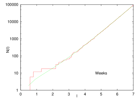
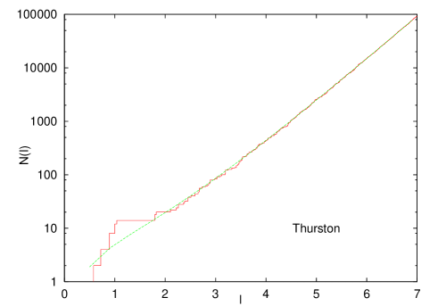
Figure 3.8: Classical Staircases

The classical staircases $N(l)$ for the Weeks manifold and the Thurston manifold are well consistent with the asymptotic distribution (3.70) for large $l$.

The topological entropy for $D$-dimensional CH spaces is given by $\tau=D-1$. A larger topological entropy implies that the efficiency in computation of periodic orbit is much less for higher dimensional cases[AM].
In figure 3.8, the computed classical staircases ($l_{cut}=7.0$) are compared with the asymptotic formula for the smallest (Weeks) manifold and the second smallest (Thurston) manifold. For both cases, an asymptotic behavior is already observed at $l\sim 3.5$.
Although the asymptotic behavior of the classical staircase $N(l)$ does not depend on the topology of the manifold, the multiplicity number $m(l)$ does. In fact, it was Aurich and Steiner who firstly noticed that the locally averaged multiplicity number

$$<\!m(l)\!>=\frac{1}{N}\sum_{l-\Delta l/2<l_{i}<l+\Delta l/2}g(l_{i}),~{}~{}~{}(N\!=\!\textrm{total number of terms})$$ (3.71)

grows exponentially $<\!m(l)\!>\sim e^{l/2}/l$ as $l\!\rightarrow\!\infty$ for arithmetic 2-spaces (manifolds and orbifolds)[BSS, AS0, ASS]. since the length $l$ of the periodic orbits are determined by algebraic integers in the form $2\cosh(l/2)=\textit{algebraic integer}$. The failure of application of the random matrix theory to some CH spaces may be attributed to the arithmetic property. For non-arithmetic spaces, one expects that the multiplicities are determined by the symmetries (elements of the isometry group) of the space. However, in the case of a non-arithmetic 3-orbifold, it has been found that $<\!m(l)\!>$ grows exponentially in the form $e^{bl}/(cl)$ where $b$ and $c$ are fitting parameters[AM]. This fact might implies that the symmetries of long periodic orbits are much larger than that of the space even in the case of non-arithmetic systems.
For 3-manifolds, one can expect that the property of $<\!m(l)\!>$ for 3-orbifold also holds. The locally averaged multiplicities $(\Delta l=0.2)$ for the smallest twelve examples which include seven arithmetic and five non-arithmetic 3-manifolds [CGHN] have been numerically computed using SnapPea.

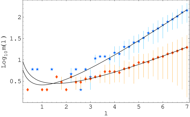
Figure 3.9: Locally Averaged Multiplicities

Plots of locally averaged multiplicities ($\Delta l=0.2$) with one-sigma errors and the fitting curves for the Weeks manifold m003(-3,1) which is arithmetic (star) and a non-arithmetic manifold m004(1,2) (diamond). The fitting curves ($a\exp(l)/l$ for the former and $\exp(bl)/(cl)$ for the latter) are obtained by the least square method using data $3.0<l<7.0$.

manifold	volume	A/N	G	$a$	$b$	$c$
m003(-3,1)	0.9427	A	D6	0.9514	-	-
m003(-2,3)	0.9814	A	D2	0.5667	-	-
m007(3,1)	1.0149	A	D2$\dagger$	0.7108	-	-
m003(-4,3)	1.2637	A	D4	0.8364	-	-
m004(6,1)	1.2845	A	D2	0.6066	-	-
m004(1,2)	1.3985	N	D2	-	0.6360	0.6180
m009(4,1)	1.4141	A	D2	0.5362	-	-
m003(-3,4)	1.4141	A	D2	0.5655	-	-
m003(-4,1)	1.4236	N	D2	-	0.5933	0.5912
m003(3,2)	1.4407	N	D2	-	0.6018	0.5532
m004(7,1)	1.4638	N	D2	-	0.5693	0.4829
m004(5,2)	1.5295	N	D2	-	0.5780	0.5590

Table 3.5: Coefficients of Fitting Curves for Averaged Multiplicities

Coefficients of the fitting curves which describe the average behavior of locally averaged multiplicities $<\!m(l)\!>$ for arithmetic (A) and non-arithmetic (N) 3-manifolds. G denotes the isometry group (symmetry group). Fitting parameters $a,b$ and $c$ are obtained by the least square method using data $3.0<l<7.0$. $\dagger$ For m007(3,1), the isometry group may be larger than D2.

From figure 3.9, one can see that the difference in the behavior of $<\!m(l)\!>$ between the non-arithmetic manifold and the arithmetic one is manifest. As observed in 3-orbifolds, averaged multiplicities behave as

$$<\!m(l)\!> = a\frac{\exp{l}}{l},~{}~{}~{}~{}~{}~{}\textrm{(arithmetic)},$$ (3.72)

$$= \frac{\exp{bl}}{cl},~{}~{}~{}~{}~{}\textrm{(non-arithmetic)},$$ (3.73)

where $a$ depends on the discrete isometry group while $b$ and $c$ are fitting parameters. From table I, one observes that arithmetic manifolds having a larger symmetry group have a larger value of $a$. The growth rates for non-arithmetic manifolds ($b\sim 0.56$) are always less than that for arithmetic manifolds ($b=1$) but nevertheless exponential.

3.2.2 Trace formula

Gutzwiller’s periodic orbit theory provides a semiclassical quantization rule for classically chaotic systems. The theory is expressed in form of a semiclassical approximation ($\hbar\rightarrow 0$) of the trace of the energy Green’s operator (resolvent operator) $\hat{G_{E}}\!=\!(\Delta+E)^{-1}$ in terms of the length of periodic orbits (geodesics) $\{L_{i}\}$ which is known as the Gutzwiller trace formula[Gutzwiller]. For the dynamical system of a free massive particle on a CH space known as the Hadamard-Gutzwiller model, the periodic orbits give the exact eigenvalues, and the relation is no longer semi-classical approximation. In mathematical literature, the trace formula is known as the Selberg trace formula [Selberg]. In what follows we consider only orientable CH 3-manifolds(denoted as CH manifolds) (for general cases including orbifolds, see [AM]). The Selberg trace formula for a CH manifold $M\!=\!H^{3}/\Gamma$ ($\Gamma$ is a discrete isometry group containing only hyperbolic or loxodromic elements) can be written as

$$Tr(\hat{G}_{E}-\hat{G}_{E^{\prime}}) = -\frac{v(M)}{4\pi i}(p-p^{\prime})$$ (3.74)

$$-\sum_{\{g_{\tau}\}}\frac{l(g_{\tau_{0}})}{4(\cosh l(g_{\tau})-\cos\phi(g_{\tau}))}\Biggl{(}\frac{\exp(-ipl(g_{\tau}))}{ip}-\frac{\exp(-ip^{\prime}l(g_{\tau}))}{ip^{\prime}}\Biggr{)},$$

where $p^{2}\!=\!E-1$, $v(M)$ denotes the volume of $M$, $l(g_{\tau})$ is the (real) length of the periodic orbit of transformation $g_{\tau}\in\Gamma$. $g_{\tau_{0}}$ is a transformation that gives the shortest length of the periodic orbit $l(g_{\tau_{0}})$ which commutes with $g_{\tau}$. $\phi(g_{\tau})$ is the phase of the transformation $g_{\tau}$. The sum in (3.74) extends over $\Gamma$ conjugacy classes

$$\{g_{\tau}\}:=\{g^{\prime}_{\tau}|g_{\tau}^{\prime}=hg_{\tau}h^{-1},h\in\Gamma\}$$ (3.75)

of hyperbolic ($\phi\!=\!0$) or loxodromic elements ($\phi\!\neq\!0$). However the periodic orbit sum in (3.74) which is known as Maaß-Selberg series converges at only complex energy such that $\textrm{Im}~{}p\!<\!-1$ and $\textrm{Im}~{}p^{\prime}\!<\!-1$. In order to obtain real eigenvalues, one needs to multiply the trace by some suitable analytic “smoothing” function $h(q)$ that satisfies:
(i):$h(q)=h(-q)$;
(ii):$h(q)={\cal{O}}(|q|^{-3-\delta})$ for $\delta>0$ as $|q|\rightarrow\infty$;
(iii):$h(q)$ is analytic in the strip ${|\textrm{Im}~{}q|<1+\epsilon}$ for $\epsilon>0$.
Multiplying (3.74) by $q~{}h(q)/(\pi~{}i)$ and integrating it over $q$ from $-\infty$ to $\infty$, one obtains the general Selberg trace formula,

$$\sum_{n=0}^{\infty}h(p_{n})= - \frac{v(M)}{2\pi}\tilde{h}^{\prime\prime}(0)$$ (3.76)

$$+ \sum_{\{g_{\tau}\}}\frac{l(g_{\tau_{0}})}{2(\cosh~{}l(g_{\tau})-\cos~{}\phi(g_{\tau}))}~{}\tilde{h}(l(g_{\tau})),$$

where

$$\tilde{h}(l)=\frac{1}{2\pi}\int_{\infty}^{\infty}dq~{}h(q)~{}\exp(-iql),$$ (3.77)

and $\tilde{h}^{\prime\prime}(0)$ is the second derivative of $\tilde{h}$ and $p_{n}$ denotes a wavenumber of the corresponding eigenmode. The sum in (3.76) is absolutely convergent for any real eigenvalues $E_{n}=p_{n}^{2}+1$. One can obtain various functions of eigenvalues such as heat kernels and energy level densities from periodic orbits by choosing an appropriate “smoothing” function $h(q)$.
In order to obtain eigenvalues, a simple approach is to compute the spectral staircase

$$N(E)=\sum_{n=0}^{\infty}\theta(E-E_{n}),$$ (3.78)

where $E_{0}\!=\!0,E_{1},E_{2},\cdots$ are the eigenvalues of the Laplacian and $\theta$ is the Heaviside function[AS1]. To explore supercurvature modes $u_{E}$, $0\leq E<1$, we choose the “smoothing” function of $N(E)$ as

$$h_{p\!,\epsilon}(p^{\prime}) = \frac{1}{2}\Biggl{(}1-\textrm{Erf}\biggl{(}\frac{E^{\prime}-E}{\epsilon^{2}}\biggr{)}\Biggr{)},$$ (3.79)

$$= \frac{1}{2}\biggl{(}1-\textrm{Erf}\biggl{(}\frac{p^{\prime 2}-p^{2}}{\epsilon^{2}}\biggr{)}\biggr{)},$$

which is real for $E>0$. Note that $h_{p}(p^{\prime})$ satisfies all the conditions (i) to (iii). By taking the limit $\epsilon\rightarrow 0$, one obtains the spectral staircase

$$N(E)=\lim_{\epsilon\rightarrow 0}\sum_{n=0}^{\infty}h_{p\!,\epsilon}(p_{n}).$$ (3.80)

Let us first estimate the behavior of the trace in (3.76). From a straightforward calculation, the zero-length contribution can be written as

$$\tilde{h}^{\prime\prime}_{p\!,\epsilon}(0)= - \frac{\epsilon^{3}}{6~{}\pi^{\frac{3}{2}}}\exp(-p^{4}/\epsilon^{4})$$ (3.81)

$$\times \biggl{(}\frac{\sqrt{2}\pi}{4}(\Gamma(3/4))^{-1}F(5/4,~{}1/2,~{}p^{4}/\epsilon^{4})+\frac{3~{}p^{2}}{2~{}\epsilon^{2}}\Gamma(3/4)F(7/4,~{}3/2,~{}p^{4}/\epsilon^{4})\biggr{)},$$

where $\Gamma(x)$ is the Gamma function and $F(a,b,z)$ is the confluent hypergeometric function. For $x\!=\!p^{4}/\epsilon^{4}\!\rightarrow\!\infty$, it is asymptotically expanded as

$$F(a,b,x) = \frac{\Gamma(b)}{\Gamma(b-a)}e^{i\pi a}x^{-a}\Biggl{\{}\sum_{n=0}^{R-1}\frac{(a)_{n}(1+a-b)_{n}}{n!}(-x)^{-n}+{\cal{O}}(x^{-R})\Biggr{\}}$$ (3.82)

$$+ \frac{\Gamma(b)}{\Gamma(a)}e^{x}x^{a-b}\Biggl{\{}\sum_{n=0}^{S-1}\frac{(b-a)_{n}(1-a)_{n}}{n!}(x)^{-n}+{\cal{O}}(x^{-S})\Biggr{\}},$$

where $(a)_{m}\equiv\Gamma(a+m)/\Gamma(a)$. From (3.81) and (3.82), in the lowest order, we have the average part,

$$\hat{N}(p)=\lim_{\epsilon\rightarrow 0}-\frac{v(M)}{2\pi}\tilde{h}^{\prime\prime}_{p\!,\epsilon}(0)=\frac{v(M)}{6\pi^{2}}|p^{2}|^{\frac{3}{2}},$$ (3.83)

that gives the dominant term in the Weyl asymptotic formula for $p\!>>\!1$.
Next, we estimate the oscillating term in (3.76)

$$\tilde{h}_{p,\epsilon}(l)=\alpha\int_{-\infty}^{\infty}dq~{}\textrm{exp}(-iql)~{}q~{}\textrm{exp}\Bigl{(}-\frac{(q^{2}-p^{2})^{2}}{\epsilon^{4}}\Bigr{)},~{}~{}~{}~{}\alpha\equiv\frac{i}{l\epsilon^{2}\pi^{3/2}}.$$ (3.84)

In the long orbit-length limit $l\!>\!>\!1$ with $p\!>\!0$, the integrand in Eq.(3.84) oscillates so rapidly that the dominant contribution comes from $q\!\sim\!p,$ or $-p$ where $(q^{2}-p^{2})^{2}/\epsilon^{4}$ can be approximately given as $-4(q-p)^{2}p^{2}/\epsilon^{4}$. Then (3.84) can be written as

$$\tilde{h}_{p,\epsilon}(l)\sim\frac{1}{\pi l}\sin(pl)\textrm{exp}\biggl{(}\frac{-\epsilon^{4}l^{2}}{16p^{2}}\biggr{)}.$$ (3.85)

Thus each periodic orbit corresponds to a wave with wavelength $2\pi/l$ and an amplitude which is exponentially suppressed with an increase in $l$ or a decrease in $p$. For a finite subset of length spectra $l_{j}<l_{cut}$, the appropriate choice for the smoothing scale is given by $\epsilon\!=\!\alpha p^{1/2}$ for $p^{2}\!>\!0$ where $\alpha$ depends on $\l_{cut}$ since for a reasonable value of the proportional factor $\alpha$ all the contributions from periodic orbits with large length $l>l_{cut}$ can be negligible. For $p^{2}\!<\!0$, an optimal choice can be obtained from a numerical computation of Eq.(3.84) directly. Comparing the obtained smoothed spectral staircase with the one based on the computed “true” eigenvalues using the direct boundary element method (DBEM), it is numerically found that for $l_{cut}\!=\!7.0$, an appropriate smoothing scale is given by

$$\epsilon(k)=\cases{0.116k^{2}+0.184~{}k+1.2~{}~{}(k<1)\cr 0.832k^{1/2}+0.668~{}~{}(k\geq 1)\cr},$$ (3.86)

where $E=k^{2}=p^{2}+1$. The eigenvalues can be computed by searching $E$ at which $N(E)-0.5$ becomes positive integer. It should be emphasized that the precision of computation depends on the value of $l_{cut}\!$ which determines the resolution scale in the eigenvalue spectra.
In order to get eigenvalues from the smoothed spectral staircase, one must take into account the effect of the multiplicity number (degeneracy number) for each eigenvalue since the spectral staircase is smoothed on larger scales for degenerate modes. Therefore, the numerical accuracy becomes worse if the eigenmode has a large multiplicity number. Fortunately, the order of the symmetry group is not so large for a small manifold (volume$<3$). For instance, of the twelve smallest examples, nine manifolds have a symmetry group with order 4. If one assumes that the multiplicity number is either 1 or 2 then the deviation $\Delta k$ from a precise value is approximately given by

$$\frac{1}{2}\Biggl{(}1-\textrm{Erf}\biggl{(}\frac{k^{2}-(k+\Delta k)^{2}}{\epsilon^{2}}\biggr{)}\Biggr{)}=\frac{1\pm 0.5}{2}.$$ (3.87)

For instance, if one uses a length spectrum $l<7.0$ then (3.87) gives $\Delta k\!=\!0.30,0.33$ for $k\!=\!5.0,3.0$, respectively. If one permits the multiplicity number as much as $6$, then the expected precision becomes $\Delta k\!=\!0.49,0.54$ for $k\!=\!5.0,3.0$, respectively.

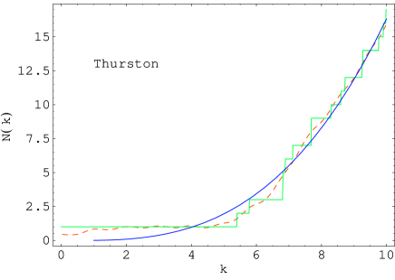
Figure 3.10: Spectral Staircases

The spectral staircases $N(k)$ for the Weeks manifold and the Thurston manifold obtained by the DBEM are compared with the average parts $\hat{N}(k)$ (solid curves), namely, Weyl’s asymptotic formula (3.83) and smoothed spectral staircase (dotted curves) obtained by the periodic orbit sum method(POSM) using all periodic orbits $l<7.0$.

manifold	volume	$k_{1}$(DBEM)	$k_{1}$(POSM)	m($k_{1}$)	$\Delta k_{1}/k_{1}$
m003(-3,1)	0.9427	5.27	5.10	1	0.03
m003(-2,3)	0.9814	5.40	5.34	1	0.01
m007(3,1)	1.0149	5.29	5.37	1	0.02
m003(-4,3)	1.2637	4.58	4.31	2	0.06
m004(6,1)	1.2845	4.53	4.35	1	0.04
m004(1,2)	1.3985	4.03	3.93	1	0.02
m009(4,1)	1.4141	5.26	4.84	2	0.08

Table 3.6: First Eigenvalues

The first (non-zero) wavenumbers $k_{1}=E_{1}^{1/2}$ are calculated using the DBEM and using the POSM for seven smallest manifolds. $k_{1}$’s agree with relative accuracy $\Delta k_{1}/k_{1}=0.01-0.08$. The multiplicity number of the first eigenmode is calculated using the DBEM.