A Black Hole in the Superluminal source SAX J1819.3-2525 (V4641 Sgr)¹

Abstract

Spectroscopic observations of the fast X-ray transient and superluminal jet source SAX J1819.3-2525 (V4641 Sgr) reveal a best fitting period of $P_{\rm spect}=2.81678\pm 0.00056$ days and a semiamplitude of $K_{2}=211.0\pm 3.1$ km s^-1. The optical mass function is $f(M)=2.74\pm 0.12\,M_{\odot}$. We find a photometric period of $P_{\rm photo}=2.81730\pm 0.00001$ days using a light curve measured from photographic plates. The folded light curve resembles an ellipsoidal light curve with two maxima of roughly equal height and two minima of unequal depth per orbital cycle. The secondary star is a late B-type star which has evolved off the main sequence. Using a moderate resolution spectrum ($R=7000$) we measure $T_{\rm eff}=10500\pm 200$ K, $\log g=3.5\pm 0.1$, and $V_{\rm rot}\sin i=123\pm 4$ km s^-1 (1$\sigma$ errors). Assuming synchronous rotation, our measured value of the projected rotational velocity implies a mass ratio of $Q\equiv M_{1}/M_{2}=1.50\pm 0.08$ (1$\sigma$). The lack of X-ray eclipses implies an upper limit to the inclination of $i\leq 70.7^{\circ}$. On the other hand, the large amplitude of the folded light curve ($\approx 0.5$ mag) implies a large inclination ($i\gtrsim 60^{\circ}$). Using the above mass function, mass ratio, and inclination range, the mass of the compact object is in the range $8.73\leq M_{1}\leq 11.70\,M_{\odot}$ and the mass of the secondary star is in the range $5.49\leq M_{2}\leq 8.14\,M_{\odot}$ (90% confidence). The mass of the compact object is well above the maximum mass of a stable neutron star and we conclude that V4641 Sgr contains a black hole. The B-star secondary is by far the most massive, the hottest, and the most luminous secondary of the dynamically confirmed black hole X-ray transients. We find that the $\alpha$-process elements nitrogen, oxygen, calcium, magnesium, and titanium may be overabundant in the secondary star by factors of two to 10 times with respect to the sun. Finally, assuming $E(B-V)=0.32\pm 0.10$, we find a distance $7.40\leq d\leq 12.31$ kpc (90% confidence). This large distance and the high proper motions observed for the radio counterpart make V4641 Sgr possibly the most superluminal galactic source known with an apparent expansion velocity of $\gtrsim 9.5c$ and a bulk Lorentz factor of $\Gamma\gtrsim 9.5$, assuming the jets were ejected during during one of the bright X-ray flares observed with the Rossi X-ray Timing Explorer.

1 Introduction

SAX J1819.3-2525 was discovered as a relatively faint X-ray source independently with the Wide Field Cameras on BeppoSAX on 1999 February 20 (in ’t Zand et al., 1999, 2000) and with the Proportional Counter Array on the Rossi X-ray Timing Explorer on 1999 February 18 (Markwardt, Swank, & Marshall, 1999). The source had two rapid and bright X-ray flares around 1999 September 15. The first flare had a peak intensity of about 4.5 Crab in the 2-12 keV X-ray band (Smith, Levine, & Morgan, 1999) and 5 Crab in 20-100 keV X-ray band (McCollough & Finger, 1999). The second peak, which came about 0.8 days later, reached intensities of 12.2 and 8 Crab in the two bands, respectively. A few days after the giant flares the source was no longer detected in X-rays [e.g. Wijnands & van der Klis (2000)].

SAX J1819.3-2525 was detected as a bright radio source (0.4 Jy) on 1999 September 16 (Hjellming et al., 2000), about 16 hours after the second X-ray flare. The radio source was marginally resolved in this first observation, indicating high expansion velocities. Thereafter, the source was detected at radio wavelengths for about three weeks. Hjellming et al. (2000) modelled the radio images and the detailed radio light curves as a combination of the ejection of a relativistic, freely expanding jet and a subsequent ejection of a more slowly decaying, optically thin jet segment. The radio observations did not resolve the moving components of the jets, so as a result one must make an assumption about when the jets were ejected in order infer the proper motion. If the jets were ejected during the brief 4.5 Crab X-ray flare, the apparent proper motion is 0.22 arcseconds per day. Hjellming et al. (2000) concluded the most likely time of the jet ejection was during the rise of the 12 Crab X-ray flare, in which case the apparent proper motion would be 0.36 arcseconds per day. These high proper motions obviously imply large velocities; an apparent proper motion of $\gtrsim 0.22$ arcseconds per day corresponds to an apparent velocity of $\gtrsim 1.28cd$, where $c$ is the velocity of light and $d$ is the distance in kpc.

SAX J1819.3-2525 was already known as an optical variable star (Goranskij, 1978), which was discovered 21 years before the first known X-ray activity. The source had a $\approx 2$ mag flare in 1978 June, and otherwise showed variability with an amplitude of up to $\approx 1$ mag about a mean level of $B\approx 14.2$ (Goranskij, 1990). In spite of differences in the classifications and variability behavior, Goranskij’s variable was confused with GM Sgr, a long-period variable star discovered by Luyten (1927). As a result, many of the papers discussing the optical counterpart of SAX J1819.3-2525 refer to GM Sgr. Hazen et al. (1999) located the plate material used by Luyten and found that Luyten’s variable GM Sgr is actually one arcminute south of Goranskij’s variable star, which is the star at the precise radio coordinates of the X-ray transient. Goranskij’s variable has been given the new variable star designation V4641 Sgr, and we shall use this name for the remainder of the paper. Goranskij (1990) assembled a quiescent light curve using 345 plates taken over a span of about 30 years with the Crimean 40 cm astrograph. He noted a periodicity at a frequency of 2.7151 cycles per day, corresponding to a double-wave period of 0.7365483 days. However, owing to severe aliasing problems, Goranskij (1990) could not rule out 1 day aliases of his preferred period. We demonstrate below that the orbital period is 2.8713 days, which is an alias of the period noted above (i.e. $1/(0.5*2.8173)\approx 0.71$ cycles per day).

A network of optical observers had noted an increase in the variability of V4641 Sgr just prior to the giant X-ray flares (Kato et al., 1999). About six days before these flares the source showed a $\approx 1$ mag modulation with a period of $\approx 2.5$ days. The optical brightness peaked at $V=8.8$ on 1999 September 15.8, and subsequently decayed rapidly to its mean quiescent level within two days. An optical spectrum obtained 1999 September 16.25 showed very strong Balmer emission lines (Djorgovski et al., 1999). The Balmer lines made an abrupt transition from emission to absorption between 1999 September 17 and 19 (Garcia, McClintock, & Callanan, 1999). A spectrum obtained 1999 September 30 (Wagner, 1999) showed only strong Balmer absorption lines and interstellar features. At the time, this was quite confusing since the quiescent counterpart was thought to be an early K-type star based on the spectrum of GM Sgr shown in Downes et al. (1995). However, in hindsight, the Balmer absorption line spectrum makes sense since we now know that Downes et al. (1995) did not observe V4641 Sgr, which in fact contains a late B star. It now appears that the quiescent optical state was reached by 1999 September 19 (i.e. about four days after the X-rays were undetectable).

It was initially thought that V4641 Sgr was relatively nearby based on two arguments. First, if the intrinsic velocity of the jet(s) observed in V4641 Sgr is similar to the velocities observed in GRO J1655-40 and GRS 1915+105 (Mirabel & Rodriguez, 1999), then the large observed proper motion of the jet observed in V4641 Sgr would imply $d\approx 500$ pc. Second, a K-star in a $\approx 0.7$ day orbit with an apparent $V$ magnitude of $\approx 13.7$ would have a distance of $\approx 1$ kpc. We demonstrate below that $d\geq 7.4$ kpc at the 90% confidence level. Thus the apparent velocity of the 0$\farcs$25 jet(s) seen several hours after the beginning of the X-ray event was $\gtrsim 9.5c$, assuming the jets were ejected at the start of the giant X-ray flare.

The galactic “microquasars” are excellent laboratories for the study of relativistic jets since they evolve orders of magnitude more quickly than the jets in quasars evolve (Mirabel & Rodriguez, 1999). V4641 Sgr is of special interest because of its very rapid X-ray flaring behavior and its extreme superluminal jets, and because the source is optically bright in quiescence ($V\approx 13.7$). In this paper we report the results of our spectroscopic observations of V4641 Sgr. The observations and basic data reductions are summarized in Section 2. In Section 3 we establish the basic orbital parameters of the system. The modelling of a high resolution spectrum and the derivation of the secondary star properties are discussed in Section 4. We discuss the astrophysical parameters of the binary system in Section 5 and discuss the implications of our results in Section 6. The paper ends with a short summary in Section 7.

2 Observations

We obtained a total of 45 spectra of V4641 Sgr between 1999 September 17 and 1999 October 16 using the FAST spectrograph (Fabricant et al., 1998) on the 1.5 m telescope at the Fred L. Whipple Observatory (FLWO) on Mount Hopkins, Arizona. The 300 g mm^-1 grating was used with a Loral $512\times 2688$ CCD. About half of the observations were taken with a 1$\farcs$5 wide slit, yielding a spectral resolution of $\approx 4.1$ Å FWHM. The other observations were taken with a 5$\farcs$0 slit, yielding a spectral resolution of $\approx 6.0$ Å FWHM. The spectra cover the wavelength range 3650-6800 Å. The exposure times were from three to ten minutes and the spectra were generally obtained under mostly clear skies with seeing between 1 and 2 arcseconds. The spectrograph slit was rotated to maintain an approximate alignment with the parallactic angle, and a wavelength calibration lamp was observed after each exposure.

As we noted above, the source was active until about 1999 September 18. All of the spectra from September 17 and 18 show a broad H$\alpha$ emission line, with a full width at zero intensity of up to $\approx 5000$ km s^-1. In contrast, the higher Balmer lines were always in absorption. By September 19, the H$\alpha$ line was also in absorption, and apparently the source was near or at its quiescent level. In the present paper we will discuss 14 spectra obtained in quiescence (i.e. between 19 September and 16 October) that were taken through the 1$\farcs$5 wide slit.

A total of forty-seven additional spectra of the source were obtained 2000 June 4-7 using the FORS1 instrument on Antu, which is the first 8.2 m telescope at the European Southern Observatory, Paranal. Thirty-seven of the spectra were taken with the 600B grism and a 0$\farcs$7 wide slit; this combination gives a spectral resolution of 4 Å FWHM and a wavelength coverage of 3366-5751 Å. The other ten spectra were taken with the 600R grism and a 0$\farcs$7 wide slit, yielding a spectral resolution of 3.2 Å FWHM and a wavelength coverage of 5142-7283 Å. The seeing was relatively poor for the VLT ($\approx 1\farcs 5$), and clouds were present on the night of June 5-6. The exposure times were from 1.5 to 4 minutes depending on the conditions. An atmospheric dispersion corrector was used, so the slit was kept at the default north-south direction. Following the standard procedure at Paranal, the flat-field and wavelength calibration exposures were obtained during the daytime hours with the telescope pointed at the zenith.

Ten additional spectra of the source were obtained 2000 June 16 and 17 with the 3.5 m New Technology Telescope (NTT) at the European Southern Observatory, La Silla, using the blue arm of EMMI. The instrumental configuration consisted of the Tek $1024\times 1024$ CCD, a 1$\farcs$0 wide slit, and the grating #11, which is a high efficiency holographic grating with 3000 “grooves” per mm (Wilson et al., 1991). The spectral resolution is 0.43 Å FWHM and the wavelength coverage is 3870.6-4032.8 Å. The slit was aligned with the parallactic angle, and a thorium-argon lamp was observed for wavelength calibration. The weather was clear June 16 and a total of eight 30-minute exposures were obtained. The conditions on June 17 were quite poor, and only two 30-minute exposures were taken.

Finally, seven additional spectra were obtained 2000 August 12 and 13 with the 4.2 m William Herschel Telescope (WHT) at the Observatorio de Roque de los Muchachos, la Palma, Spain. The instrumental configuration was the blue arm of the ISIS double beam spectrograph, the R1200B grating, and the EEV12 $4096\times 2048$ CCD. We used a 0$\farcs$8 wide slit, yielding a spectral resolution of 0.58 Å FWHM and a coverage of 3680-4500 Å. The slit was aligned with the parallactic angle, and a copper-argon lamp was observed for wavelength calibration. The weather was photometric, and the seeing was generally 1$\farcs$1 or less.

We reduced all of the spectra using IRAF. The standard tasks were used to apply the bias and flat-field corrections, and to extract and wavelength-calibrate the spectra. The bright night sky emission line at $\approx 5578$ Å was used to make small adjustments to the wavelength scales of the FLWO and VLT spectra. The shifts required to align this feature to a common wavelength (5578.0 Å) were generally less than $\approx 15$ km s^-1, although the VLT spectra from the end of the night of June 7 required shifts on the order of 80 km s^-1.

Figure 1: (a): The solid line shows the reduced $\chi^{2}_{\nu}$ for a three-parameter sinusoid fit to the 71 radial velocities as a function of the trial period in days. The minimum $\chi^{2}_{\nu}$ is at $P=2.8177\pm 0.0005$ days. (b): The solid line shows the Lomb-Scargle periodogram of the photometric light curve. Peaks above the dashed line are significant at the $3\sigma$ level. The peak with the most power is at $P=1.40865$ days, which is half of the spectroscopic period. (c): The Stellingwerf (1978) $\Theta$ statistic as a function of the trial period near 2.8 days. The minimum $\Theta$ and hence the most coherent modulation is at $P=2.81730\pm 0.00001$ days. (d): An expanded view of the curve in (a). The various aliases of the spectroscopic period are ruled out by the photometry.

3 Orbital Period and Spectroscopic Elements

3.1 Spectroscopic Period

We measured the radial velocities of the secondary star using the fxcor task within IRAF, which is an implementation of the technique of Tonry & Davis (1979). Synthetic spectra with $T_{\rm eff}=10500$, $\log g=3.5$, and $V_{\rm rot}\sin i=123$ km s^-1 (see below) were used as templates for the five different sets of spectra (i.e. FLWO, VLT “blue”, VLT “red”, NTT, and WHT). The cross correlation regions covered the available wavelengths between 3700 and 6847 Å, excluding the interstellar Ca II H and K and Na D lines, the diffuse interstellar bands near 4330 and 5780 Å, and a telluric feature near 6280 Å. The final velocities for the FLWO, the VLT blue, and WHT spectra were insensitive to the exact starting and ending points of the cross correlation regions and to the function used to find the centroid of the cross correlation peak. On the other hand, the velocities of the VLT red spectra and the NTT spectra were sensitive to these parameters since these spectra contain very few lines. We can estimate approximate velocity corrections for the VLT red and NTT spectra by using observations of an A0 template star observed both with the VLT and NTT. However, we find that including the corrected velocities did not improve the resulting spectroscopic parameters since the corrected velocities all have relatively large uncertainties. We therefore excluded the VLT red and NTT velocities from the analysis presented below.

To search for the spectroscopic period we computed a three-parameter sinusoid fit to the velocities for a range of trial periods between 0 and 5 days and recorded the values of the reduced $\chi^{2}$ for the fits. The free parameters at each trial period are the velocity semiamplitude $K_{2}$, the epoch of maximum velocity $T_{0}$(spect), and the systemic velocity $\gamma$. The error bars on the individual velocities were scaled by a factor of 2.65 to yield $\chi^{2}_{\nu}=1.0$ at the minimum. Fig. 1a shows the resulting $\chi^{2}_{\nu}$ vs. $P$ curve. The best fit is at a period of $P=2.81678\pm 0.00056$ days ($1\sigma$ error). The next best fit occurs at $P=2.699$ days, where $\chi^{2}_{\nu}=2.27$. This alias period and the others are clearly ruled out by inspection of the folded velocity curves and we adopt the following spectroscopic elements: $P_{\rm spect}=2.81678\pm 0.00056$ days, $K_{2}=211.0\pm 3.1$ km s^-1, $\gamma=107.4\pm 2.9$ km s^-1, and $T_{0}({\rm spect})={\rm HJD~{}}2,451,442.523\pm 0.052$. The resulting optical mass function is then $f(M)=2.74\pm 0.12\,M_{\odot}$ ($1\sigma$ errors). Fig. 2 shows the velocities and the best fitting sinusoid, and the spectroscopic elements are listed in Table 1.

3.2 Photometric Period

Goranskij (1990) published a light curve of V4641 Sgr obtained from 345 plates taken with the Crimean 0.40 m astrograph between about 1960 and 1990. After it was realized that V4641 Sgr was the optical counterpart of SAX J1819.2-2525, Goranskij reanalyzed the photographic data and made them publically available via the VSNet. We searched these data for periodicities using both the technique of Stellingwerf (1978) and the Lomb-Scargle Periodogram (Lomb, 1976; Scargle, 1982). We excluded the uncertain measurements and also data from 1978 June, when the source had an optical flare. Fig. 1b shows the Lomb-Scargle periodogram in the period range of 0 to 5 days. Using a Monte Carlo procedure, we computed the power above which the peaks are significant at the $3\sigma$ level. We made 10,000 simulated light curves having the same observation times as the actual light curve and with magnitude points normally distributed about the mean magnitude. (By construction, the simulated light curves have the same variance as the actual light curve.) A Lomb-Scargle periodogram was computed for each simulated light curve and the power of the strongest peak was recorded. The $3\sigma$ threshold was then determined from the cumulative distribution of the peak powers. This threshold is shown by the dashed line in Fig. 1b. There are several peaks significant at the $3\sigma$ level. The peak with the most power is at a trial period of $P=1.40865$ days (0.7099 cycles day^-1), which is half of the spectroscopic period. All of the other significant peaks are aliases of the main peak (e.g. $1/1-1/1.40865=1/3.447$, etc.) and their sidebands. Fig. 1c shows the $\Theta$ statistic of Stellingwerf (1978) plotted as a function of the trial period in the range $2.6\leq P\leq 3.1$ days (we used 20 phase bins of width 0.05 to compute the $\Theta$ statistic—this combination yielded the smoothest minima). The minimum $\Theta$ is at a period of $P=2.81730$ days. Yearly aliases of this period are also evident. Fig. 1d shows the $\chi^{2}_{\nu}$ vs. $P$ curve from Fig. 1a plotted over the same period range as in Fig. 1c. The period of $P=2.81730$ days is the only trial period where there are minima in both the $\Theta$ statistic and in the $\chi^{2}_{\nu}$ vs. $P$ curve. Thus the photometric and spectroscopic periods of V4641 Sgr are nicely consistent with each other.

Figure 2: The radial velocities for V4641 Sgr folded on the spectroscopic period and phase and the best fitting sinusoid. See Table 1 for the parameters. Each point has been plotted twice for clarity.

Figure 3: The photometric light curve of V4641 Sgr folded using $P=2.81730$ days and $T_{0}=T_{0}$(photo)$+P/2$ and binned into 20 bins of equal size. Each point has been plotted twice for clarity. The error bars on the points represent the error of the mean. The solid curve is a $B$-band ellipsoidal model with $i=70^{\circ}$, $Q=1.6$, and a grazing eclipse of the star by an accretion disk. The dash curve is the resulting light curve when the disk is removed.

We computed the uncertainty in the photometric period by using another Monte Carlo procedure. We adopted a mean photometric error of 0.1 mag (Goranskij, private communication) and constructed 10,000 simulated data sets by assigning a new magnitude to each time using $y_{{\rm new},i}=y_{i}+0.1\sigma$, where $\sigma$ is a random Gaussian deviate with variance of unity and a zero mean. For each simulated data set we computed the Lomb-Scargle periodogram and the Stellingwerf $\Theta$ statistic and recorded the resulting derived periods. The uncertainty in the photometric period was taken to be the standard deviation of the distribution of best periods from these simulated data. We find $P=2.81730\pm 0.00001$ days. Fig. 3 shows the light curve folded on this period and binned into 20 phase bins. The light curve resembles an ellipsoidal light curve with two maxima of roughly equal heights and two minima of unequal depths per orbital cycle. The amplitude is quite large; the range is about 0.5 mag from the deeper minimum to the maximum.

Goranskij (1990) gives the time of minimum light $T_{0}$(photo) as HJD 2,447,707.454 (no error is quoted). We measured $T_{0}$(photo) by folding the light curve on a dense grid of trial values of $T_{0}$(photo) and recording the $\chi^{2}$ of an ellipsoidal model fit (the solid line in Fig. 3). The result is $T_{0}$(photo) = HJD 2,447,707.$4865\pm 0.0038$. The photometric phase of the time of maximum velocity $T_{0}$(spect) is $0.75\pm 0.02$, exactly as expected for an ellipsoidal light curve. (Note that the phase zero point used in Fig. 3 is $T_{0}$(photo)$+0.5P$ to conform with our ellipsoidal modelling code.)

4 Parameters for the Secondary Star

Figure 4: (a): The reduced $\chi^{2}$ as a function of the input value of $V_{\rm rot}\sin i$ for the August 13 WHT restframe spectrum (solid line) and August 12 WHT restframe spectrum (dashed line), computed using the model spectra broadened by SYNPLOT. (b): The reduced $\chi^{2}$ as a function of the input value of $V_{\rm rot}\sin i$ for the August 13 WHT restframe spectrum (solid line) and August 12 WHT restframe spectrum (dashed line), computed using the numerical broadening kernels.

Figure 5: Top: The solid line is a numerical rotational broadening kernel which is the mean of 5 separate kernels matched to the August 13 WHT spectra, scaled by 125 km s^-1. The dashed line is the analytic kernel used by SYNPLOT, scaled by 118 km s^-1. Bottom: The solid line is a numerical rotational broadening kernel which is the mean of the two separate kernels matched to the August 12 WHT spectra, scaled by 130 km s^-1. The dashed line is the analytic kernel used by SYNPLOT, scaled by 118 km s^-1.

V4641 Sgr is relatively bright, and as a result one can easily obtain a spectrum with a relatively high signal-to-noise ratio (SNR) and high resolution. The eight NTT spectra from June 16 were Doppler shifted to zero velocity and combined to yield a “restframe” spectrum with a resolution of $R=9000$ and a SNR of about 50 per pixel. In the same way, we also made a restframe spectrum using the WHT data. The SNR of the WHT restframe spectrum is about 130 per pixel and is reasonably constant over much of the spectrum. We used synthetic spectra generated from solar metallicity Kurucz models to determine three basic parameters for the secondary star, namely its effective temperature $T_{\rm eff}$, surface gravity $\log g$, and mean projected rotational velocity $V_{\rm rot}\sin i$. The IDL program SYNPLOT (Hubeny, Lanz, & Jeffrey, 1994) was used to compute the detailed model spectra. SYNPLOT can generate an optical spectrum with arbitrary spectral resolution, wavelength sampling, and rotational broadening. [Currently SYNPLOT uses an analytic broadening kernel with a linear limb darkening coefficient of $\epsilon=0.6$ (Gray, 1992)]. For the NTT spectrum the resolution was taken to be $0.4333$ Å and the wavelength sampling was 0.1530 Å, and for the WHT spectra those quantities were 0.5802 Å and 0.2231 Å, respectively. We also have two synthetic spectra kindly provided by Peter Hauschildt computed using his PHOENIX code (Hauschildt & Baron, 1999). These models are fully line-blanketed with magnesium and iron computed in non-LTE (NLTE).

We used the technique outlined in Marsh, Robinson, & Wood (1994) to fit the model spectra to the observed ones. This fitting procedure has the advantage that it allows for the possibility of a (continuum) contribution from the accretion disk. The restframe spectra were normalized to their continuum fits. An input model spectrum characterized by the three parameters $T_{\rm eff}$, $\log g$, and $V_{\rm rot}\sin i$ is normalized to its continuum using the same procedure used for the observed spectra: it is scaled by a weight factor $w$, and subtracted from the observed spectrum. The scatter in the difference spectrum is measured by computing the reduced $\chi^{2}$ from a low-order polynomial fit (after the interstellar lines were masked out of the fit). We varied $T_{\rm eff}$, $\log g$, and $V_{\rm rot}\sin i$ and looked for the “smoothest” difference spectrum. The Kurucz grid has models for gravities of $\log g=3.0$, 3.5, and 4.0 (cgs units) near the temperatures of interest (about 10000 K).

4.1 Effective Temperature and Spectral Classification

It quickly became clear using the NTT spectrum that the gravity of the secondary star in V4641 Sgr is quite close to $\log g=3.5$ since the $\log g=3.0$ models have Balmer lines that are much too narrow and the $\log g=4.0$ models have Balmer lines that are much too broad. We therefore fixed the gravity at $\log g=3.5$. The temperature is best constrained by the WHT spectrum. The He I line at 4024 Å is somewhat sensitive to the temperature, and we find $T_{\rm eff}=10500$ K. The statistical errors in the temperature and gravity are much smaller than the respective grid spacings (0.5 dex in $\log g$ and 250 K in $T_{\rm eff}$). No doubt there are systematic errors as well, but it is beyond our present ability to quantify these errors. We conservatively adopt $\sigma_{T}=200$ K and $\sigma_{\log g}=0.1$. The values of $T_{\rm eff}$ and $\log g$ we find for V4641 Sgr are not too different from those of the B9 III MK spectral type standard $\gamma$ Lyr for which Künzli et al. (1997) list $T_{\rm eff}=9970\pm 540$ and $\log g=3.50$; the gravity was estimated from a measurement of the H$\beta$ index (Balachandran et al., 1986). We fit synthetic spectra to the observed spectrum of $\gamma$ Lyr (obtained with the WHT) and find $T_{\rm eff}=10000$ K, in good agreement with the previous values, and $\log g=3.0$, somewhat lower than the previous values. Based on this approximate similarity, we assign a B9III classification to the secondary star in V4641 Sgr. We note that the spectral type of B9III derived here is somewhat earlier than the preliminary type of A2V we announced in IAU Circular 7440. The latter value was arrived at via a visual inspection of the Balmer lines in a low resolution spectrum. We believe the spectral type of B9III derived here is much more reliable since we used an impartial fitting procedure on a spectrum with higher resolution and a higher SNR.

Figure 6: The results of our exploratory abundance analysis for V4641 Sgr. We show the solar abundance base Kurucz model, and the models with the abundance patterns altered to approximately match the line profiles. The observed spectrum is from the WHT (resolution 0.58 Å FWHM). The spectrum was rebinned by a factor of 2.6 for comparison with the Ca II line and the O I line. The interstallar Ca II lines are labelled with “IS”.

Figure 7: The abundance analysis for $\gamma$ Lyr. We show the solar abundance base Kurucz model ($T_{\rm eff}=10000$ K, $\log g=3.0$), and $V_{\rm rot}\sin i=88$ km s^-1, and the models with the abundance patterns found from the V4641 Sgr spectrum. The observed spectrum is from the WHT (resolution 0.58 Å FWHM).

Figure 8: The Mg II $\lambda$4481.22 lines in V4641 Sgr (left) and $\gamma$ Lyr (right), observed with the WHT (resolution 0.58 Å FWHM). The synthetic spectra made from the LTE solar metallicity Kurucz models are shown as the dashed lines and the Hauschildt model spectra (computed with magnesium in NLTE) are shown as the solid lines. The NLTE treatment of magnesium in $\gamma$ Lyr changes the strength of the line significantly, whereas there is little change in the line strength in V4641 Sgr.

Figure 9: (a): The restframe spectrum of V4641 Sgr observed with the VLT FORS1 and grism 600B (spectral resolution 4 Å FWHM), the solar abundance model ($T_{\rm eff}=10500$ K, $\log g=3.5$, and $V_{\rm rot}\sin i=123$ km s^-1), and the Mg and Ti enhanced models. b: The restframe spectrum of V4641 Sgr observed with the VLT FORS1 and grism 600R (spectral resolution 3.2 Å FWHM), the solar abundance model ($T_{\rm eff}=10500$ K, $\log g=3.5$, and $V_{\rm rot}\sin i=123$ km s^-1), and the N, O, and Mg enhanced models

4.2 Rotational Velocity of the Secondary

Two other interesting facts also came to light in this process. First, it was apparent that the rotational velocity of V4641 Sgr is quite high ($\gtrsim 0.5K_{2}$) since the atomic lines are quite broadened by rotation. Second, some of the metal lines (most noteably Mg II near 4781 Å) are much stronger in V4641 Sgr than they are in the models. We therefore iterated the fits to determine the rotational velocity and the approximate abundances of Mg and other metals.

Figure 10: (a): The restframe WHT spectrum of V4641 Sgr, normalized to its continuum and offset upwards by 2.0 units. (b): A synthetic spectrum with $T_{\rm eff}=10500$ K, $\log g=3.5$, and $V_{\rm rot}\sin i=123$ km s^-1 offset by 1.5. (c): A synthetic spectrum with $T_{\rm eff}=10500$ K, $\log g=3.5$, and $V_{\rm rot}\sin i=1$ km s^-1, not offset. (d): The observed spectrum minus the $T_{\rm eff}=10500$ K, $\log g=3.5$, and $V_{\rm rot}\sin i=123$ km s^-1 model, no offset. (e). The observed $\gamma$ Lyr spectrum minus the best fitting model ($T_{\rm eff}=10000$ K, $\log g=3.0$, and $V_{\rm rot}\sin i=88$ km s^-1), offset downwards by 0.4 units.

We started first with the determination of the rotational velocity. We computed model spectra for various values of $V_{\rm rot}\sin i$ (using $T_{\rm eff}=10500$ K and $\log g=3.5$) and computed the minimum reduced $\chi^{2}$ of the polynomial fit to the difference spectra, masking out the few anomalous lines. It is well known that there is a systematic error in the measurement of $V_{\rm rot}\sin i$ caused by the non-spherical shape of the Roche lobe and by the variations in the temperature and limb darkening over the Roche surface. Therefore we made nightly restframe spectra using the two WHT spectra from August 12 and the five WHT spectra from August 13, thus insuring that the restframe spectra are composed of individual spectra with similarly distorted line profiles. Fig. 4a shows the reduced $\chi^{2}$ as a function of the input $V_{\rm rot}\sin i$ for the two restframe spectra. The minimum reduced $\chi^{2}$ for the August 13 spectrum (which has the larger SNR) is for $V_{\rm rot}\sin i=118$ km s^-1. However, the curve is somewhat noisy, and there is another dip near $V_{\rm rot}\sin i=113$ km s^-1. The corresponding curve for the August 12 restframe spectrum has its minimum at $V_{\rm rot}\sin i=124$ km s^-1, and another broad minimum near $V_{\rm rot}\sin i=130$ km s^-1.

It is somewhat difficult to choose the correct value of $V_{\rm rot}\sin i$ on the basis of these results. We repeated the exercise using phase-specific broadening kernels, computed using the ELC code (Orosz & Hauschildt, 2000). The ELC code uses specific intensities from model atmosphere computations rather than from blackbodies and a one- or two-parameter limb darkening law. Thus the distortions in the broadening kernel due to tidal distortions and to temperature and limb darkening variations are accounted for in detail. For the present problem we used the specific intensities from the Kurucz grid. We computed a broadening kernel for each of the two nights by averaging kernels made for each individual spectrum which went into the restframe average. We used a custom made IRAF routine to compute the convolution. Fig. 4b shows the resulting reduced $\chi^{2}$ vs. $V_{\rm rot}\sin i$. The two curves are much “cleaner”, and both have well-defined minima near $V_{\rm rot}\sin i=123$ km s^-1. Fig. 5 shows the numerical kernels used. In the case of the August 13 spectrum, the analytic kernel scaled by 118 km s^-1 has almost the same full width at half maximum as the slightly asymmetric numerical kernel, scaled by 123 km s^-1. Thus, to first order, we would expect a correction from 118 to 123 km s^-1, which is what we find. Similarly, the analytic kernel scaled by 130 km s^-1 approximately matches the full width at half maximum of the numerical kernel for August 12, scaled by 123 km s^-1. Thus we adopt $V_{\rm rot}\sin i=123$ km s^-1. The curves in Fig. 4b start to become steep at $\approx 119$ and 127 km s^-1, so we adopt a $1\sigma$ error of 4 km s^-1.

4.3 Abundance Anomalies

After determining the rotational velocity we then examined in more detail the metal lines that were unexpectedly strong. SYNPLOT can alter the abundance of any given element and compute an approximate line profile. The resulting line profile is reasonably accurate provided the abundance of the element in question is not altered by more than a factor of $\approx 3$ from its abundance in the input model atmosphere (I. Hubeny, private communication). Since we currently cannot compute a full grid of the fully line-blanketed Kurucz models with arbitrary abundance patterns, our results should be taken as only indicative. We computed models with altered abundances and compared them to the observed V4641 Sgr spectrum. In searching for elements with possible abundance anomalies, we were guided by the work of Israelian et al (1999) who found that the abundances of the $\alpha$-process elements nitrogen, oxygen, magnesium, silicon, and titanium in the F-star secondary of GRO J1655-40 are 6-10 times solar. We concentrated on these same elements in V4641 Sgr. As a check, we also computed models for $\gamma$ Lyr with altered abundances. The results are given in Table 2 and in Figs. 6, 7, and 9. Details for each element are provided below.

Taken at face value, the LTE Kurucz models indicate that the magnesium in V4641 Sgr is enhanced by about a factor of five to seven with respect to solar. However, we cannot fit the magnesium lines in $\gamma$ Lyr using the LTE Kurucz models (Fig.7), which is an indication that a NLTE treatment is needed. In Figure 8 we show the Kurucz models and the Hauschildt models for V4641 Sgr and $\gamma$ Lyr near the Mg II $\lambda$4481.22 line. In the case of V4641 Sgr ($T_{\rm eff}=10500$, $\log g=3.5$), the NLTE treatment makes almost no difference to the strength of the $\lambda$4481.22 line. In contrast, the NLTE treatment makes the $\lambda$4481.22 line much stronger in $\gamma$ Lyr ($T_{\rm eff}=10000$, $\log g=3$). We conclude the unusual strength of the $\lambda$4481.22 line in V4641 Sgr is due to an enhancement of magnesium of a factor of five to seven times solar.

The pair of lines at $\lambda$4128.04 and 4130.58 due to Si II indicates roughly solar abundance in V4641 Sgr; but as with magnesium, these Si II lines are not well modelled in $\gamma$ Lyr. NLTE effects probably are important for Si II as well.

Perhaps the most convincing case is for oxygen. The weak O I line at $\lambda$4368.2 observed in V4641 Sgr requires an oxygen enhancement of 3 times solar, whereas the solar abundance model for $\gamma$ Lyr fits the line profile in that star. For comparison, Balachandran et al. (1986) measured an oxygen abundance in $\gamma$ Lyr of about 1.3 times solar. The unresolved O I triplet near $\lambda$6454.4 appears in the VLT spectrum (resolution 3.2 Å FWHM, Fig. 9). Its strength suggests the abundance is even a bit more than three times solar (we did not attempt any further iteration, given the low resolution of the VLT spectrum).

The stellar Ca II line at $\lambda$3933.66 in V4641 Sgr was resolved from the interstellar line in the August 12 WHT spectrum. A calcium enhancement of twice solar is needed to fit the line. The Ca II line in $\gamma$ Lyr is fit by the solar abundance model.

There are no strong titanium lines that are sensitive to the abundance in the WHT spectrum. The VLT spectrum (resolution 4 Å FWHM) contains two Ti II lines that appeared to be much stronger than the corresponding model lines (Fig. 9). A titanium enhancement of a factor of about 10 can explain the profiles of the $\lambda 5226.5$ and $\lambda$5129.2 lines, but not the blend at $\approx\lambda$5187.

There are no strong nitrogen lines in the WHT spectrum. There is a line due to N I in the VLT spectrum (resolution 3.2 Å FWHM) which is anomolous. A model with a nitrogen enhancement of a factor of 10 solar gives a reasonably good fit to the profile. We also searched the WHT and VLT spectra for suitable sulphur lines, but we did not find any.

To summarize the results of our exploratory abundance analysis, we find the following enhancements: nitrogen is $\approx 10$ times solar (low resolution spectrum only); oxygen is $\approx 3$ times solar (low and high resolution spectra); magnesium is enhanced by about five to seven times solar; silicon is roughly solar, but the LTE models may not be adequate; calcium is $\approx 2$ times solar (high resolution spectrum); and titanium is $\approx 10$ times solar (low resolution spectrum only). As we stated above, these results should be treated with extreme caution. We do not claim that the lines we examined are the most suitable ones for an abundance analysis, nor do we claim the solar metallicity Kurucz models are the most appropriate. Clearly we need better data (e.g. higher resolution spectra with lines from more than one ionization stage of the elements in question) and better models (e.g. NLTE treatment for all of the elements, etc.).

Finally, we repeated the procedure to find the rotational velocity, using a model with altered oxygen, magnesium, and calcium abundances. We found no change in the value of $V_{\rm rot}\sin i$. Fig. 10 shows the normalized WHT spectrum, the best (normalized) model, and the difference between the two. The agreement between the model and the data is quite good. The accretion disk is faint; it contributes less than 1% of the light. For comparison, we also show the difference between the model for $\gamma$ Lyr and the observed spectrum (spectrum e).

5 Astrophysical Parameters

Now that we have presented the observational facts concerning V4641 Sgr, we proceed to discuss the astrophysical implications of these observations.

5.1 Inclination Constraints

A straightforward upper limit to the inclination comes from the lack of X-ray eclipses. As we noted earlier, the source was active as a relatively weak X-ray source between 1999 February and September and was detected on numerous occasions by the PCA instrument on RXTE. C. Markwardt (private communication) informs us that the source was detected in X-rays several times near the inferior conjunction of the secondary star (i.e. a spectroscopic phase range of $0.75\pm 0.04$). Assuming the X-rays come from a relatively small region $R\lesssim 0.01\,R_{\odot}$ centered on the compact object, one can show $i\leq 70.7^{\circ}$ for $Q=1.5$.

In principle, one can determine the inclination by modelling the so-called “ellipsoidal” variations in the light curve of the B-star companion. The B-star fills its critical Roche lobe (there is ongoing mass transfer) and as such is quite distorted. As the distorted star moves about in its 2.8173 day orbit, the projected area on the sky changes, which in turn, gives rise to changes in the observed flux. The net result is that one observes a light curve with two maxima per cycle (corresponding to the quadrature phases when the star is seen “side-on”) and two minima per cycle (when the star is seen “end-on”). The amplitude of the light curve and the details of its shape is a function of the inclination.

In practice, however, there are difficulties which can introduce systematic errors into the ellipsoidal modelling. For example, the accretion disk can contribute a significant amount of flux, thereby “diluting” the ellipsoidal light curve observed from the secondary. From an empirical point of view, the black hole binaries with cool companions (G, K, or M-type companions) are subject to the biggest systematic uncertainties since their light curves change from one observing run to the next (McClintock & Remillard, 1986; Orosz et al., 1996; Haswell et al., 1993; Webb et al., 2000). On the other hand, the two black hole binaries with hot companions (GRO J1655-40 with an F6III companion and 4U 1543-47 with an A2V companion) have light curves which are quite stable, and it is apparent that the underlying ellipsoidal light curve of the secondary star dominates in these two cases. The light curves of GRO J1655-40 have been recently modelled and reasonably tight inclination constraints (to within about 5 degrees at 90% confidence) have been obtained (Greene, Bailyn, & Orosz 2000). Since V4641 Sgr contains a hot companion, it seems reasonable to expect that its light curve will be dominated by the ellipsoidal modulations from the secondary.

The only well-sampled light curve we have access to at the moment is the photometric light curve assembled by Goranskij (1990). Unfortunately, the individual measurements are relatively imprecise (the mean estimated error is 0.1 mag), and the folded and binned light curve (Fig. 3) has relatively large error bars. Nevertheless, the ellipsoidal modulation is apparent in the binned light curve. For the moment we will limit ourselves to some representative models and put off the more detailed modelling until precise CCD light curves in several filter bandpasses become available. We used the ELC code (Orosz & Hauschildt, 2000) to compute the models using specific intensities from the Kurucz grid. The dashed line in Fig. 3 is a Johnson $B$-band model for a lobe-filling star ($T_{\rm mean}=10500$ K) with an inclination of $i=70^{\circ}$ and a mass ratio of $Q=1.5$. The amplitude of the model is too small ($\chi^{2}=35.196$ for the 20 data points). The solid line in Fig. 3 is the same model, but with a faint accretion disk added (the outer radius is 98% of the Roche lobe radius). The depth of the minimum at phase 0.5 is increased by the partial eclipse of the B-star by the disk. In this case, the amplitude of the model is much closer to what is observed, and the model fit is improved ($\chi^{2}=25.39$ for the 20 data points). The model disk contributes about 0.25% of the light in the $B$-band, and this would be compatible with the observed limits (Sec. 4). To find an approximate lower limit to the inclination, we adjusted the inclination of the model until the $\chi^{2}$ of the fit increased by 9. The mass ratio and the radius of the disk were not adjusted. We find $i\gtrsim 60^{\circ}$.

We adopt an inclination range that is uniform in the interval $60^{\circ}\leq i\leq 70.7^{\circ}$. A partial eclipse of the secondary star is needed to reproduce the relative depths of the minima. These conclusions (apart from the upper limit on $i$ which is a function of $Q$ only) should be treated with caution, given that the light curve is relatively uncertain.

5.2 Binary Parameters

Figure 11: Top: The radius of the secondary star as a function of its assumed mass. The points are from the single star Geneva stellar evolution models. Middle: Similar to the top, except the luminosity of the secondary star is displayed. Bottom: The distance of the source (right $y$-axis scale) and the peak isotropic X-ray luminosity (left $y$-axis scale) as a function of the assumed secondary star mass for three different values of the color excess. The photometry of the source in quiescence suggests $E(B-V)=0.32$.

For a Roche lobe filling star it is straightforward to show that

$${V_{\rm rot}\sin i\over K_{2}}={R_{L_{1}}(Q)\over a}\left({1+Q\over Q}\right),$$ (1)

where $Q$ is the mass ratio, $R_{L_{1}}(Q)$ is the sphere-equivalent radius of the Roche lobe, and $V_{\rm rot}=2\pi R_{L_{1}}/P$. We used the ELC code to numerically compute $R_{L_{1}}(Q)$ for $V_{\rm rot}=123\pm 5$ km s^-1 and $K_{2}=211.0\pm 3.1$ km s^-1; we find $Q=1.50\pm 0.13$ (90% confidence).

We used a simple Monte Carlo code to compute other interesting binary parameters (e.g. the component masses, secondary star radius, etc.) and their uncertainties using four input quantities, namely the period ($P=2.81730\pm 0.00001$ days, $1\sigma$), the velocity semiamplitude of the secondary star ($K_{2}=211.0\pm 3.1$ km s^-1, $1\sigma$), the projected rotational velocity of the secondary star ($V_{\rm rot}\sin i=123\pm 4$ km s^-1, $1\sigma$), and the inclination ($60.0^{\circ}\leq i\leq 70.7^{\circ}$, uniform distribution). The nominal masses of the black hole and secondary star are $9.6\,M_{\odot}$ and $6.5\,M_{\odot}$, respectively; the precise masses and other key results are summarized in Table 3.

6 Discussion

The mass of the compact object in V4641 Sgr ($9.6\,M_{\odot}$) is well above the maximum mass of a stable neutron star, which is usually taken to be $\approx 3\,M_{\odot}$ (Chitre & Hartle, 1976). We therefore conclude that V4641 Sgr contains a black hole. V4641 Sgr is also interesting in several other respects. The B-star secondary is by far the most massive, the hottest, and the most luminous secondary of the ten dynamically confirmed transient black hole binaries. The total mass of the system, $16.2\,M_{\odot}$, is also largest among the dynamically confirmed black hole binaries. The next most massive system is V404 Cyg whose total mass is about $12.7\,M_{\odot}$ (Shahbaz et al., 1994). The other eight confirmed transient black hole binaries have total masses which are probably below $10\,M_{\odot}$, although the uncertainties are large in many cases (Bailyn et al., 1998, and cited references).

The secondary star in V4641 Sgr appears to be in an unusual evolutionary state. To help illustrate this, we plot in Fig. 11ab the radius of the secondary and the luminosity of the secondary as a function of its assumed mass. Since the density of a Roche lobe filling star depends only on the orbital period of the binary to a good approximation, these curves are essentially independent of the inclination or the mass ratio of the binary. We also show the radius and luminosity of single stars, taken from the “Geneva” stellar evolution models (Schaller et al., 1992). For our adopted mass range of $5.49\leq M_{2}\leq 8.14\,M_{\odot}$ (90% confidence), the secondary star is both smaller in size and significantly underluminous compared to single stars of similar masses. An underluminous secondary star usually indicates that the star went through a phase of thermally unstable mass transfer. A more detailed discussion of the evolutionary history of this star is beyond the scope of the current paper.

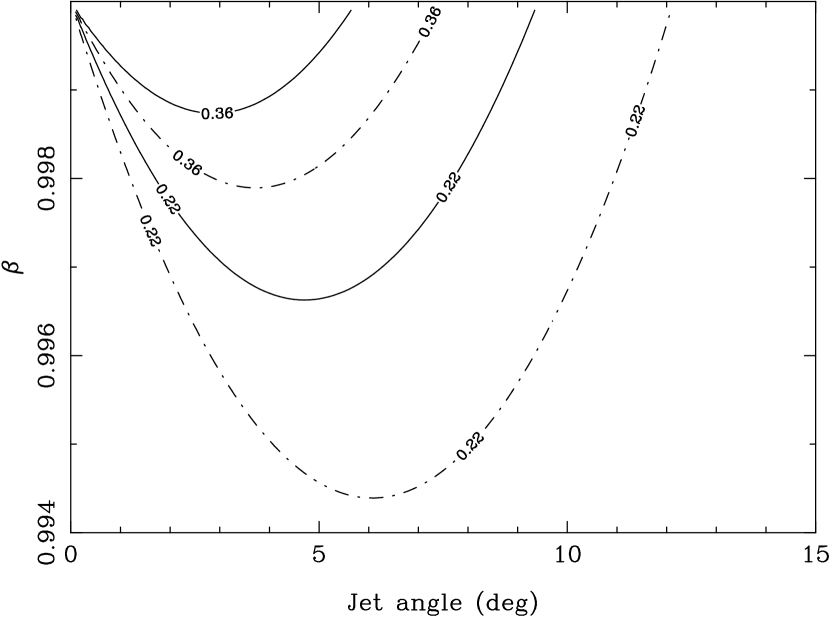
Figure 12: A contour plot of the apparent proper motion in arcseconds per day of the approaching jet in V4641 Sgr as a function of the jet angle and the intrinsic jet velocity in units of $c$. The dash countours are for a distance of 7.4 kpc and the solid contours are for a distance of 9.6 kpc.

Two remarkable features of V4641 Sgr, which are discussed below, are a consequence of its great distance. For an assumed secondary star mass, we know precisely the corresponding radius. The corresponding luminosity is also precisely known since the temperature is well known from the spectrum. The distance then follows from the apparent $V$ magnitude and the extinction. Photometry of the source was obtained from CTIO 2000 July 23.1 (UT). We find $B=14.00\pm 0.02$ and $V=13.68\pm 0.02$. The intrinsic colors of this star are all close to zero, hence $E(B-V)=0.32$. The star is of course variable, so for now we adopt an uncertainty on the $B$ and $V$ magnitudes of 0.1 mag. Fig. 11c shows the distance as a function of the assumed secondary star mass. Assuming $T_{\rm eff}=10500\pm 200$ K and $5.49\leq M_{2}\leq 8.14\,M_{\odot}$ (90% confidence), we adopt $7.40\leq d\leq 12.31$ kpc (90% confidence).

As we noted earlier, V4641 Sgr was marginally resolved in the first radio map made after the 12 crab X-ray flare. The proper motion of the jet is uncertain since it is not known when the jet was ejected. Hjellming et al. (2000) give three possibilities for the jet proper motion, based on known X-ray/radio correlations in other sources:

• $\mu_{\rm jet}=0.22$ arcseconds per day for an ejection at the start of the 4.5 crab X-ray flare, which implies $V_{\rm app}\geq 9.47c$ for $d>7.4$ kpc;

• $\mu_{\rm jet}=0.36$ arcseconds per day for an ejection at the start of the 12 crab X-ray flare (this is their preferred value), which implies $V_{\rm app}\geq 15.4c$ for $d>7.4$ kpc;

• $\mu_{\rm jet}=1.1$ arcseconds per day for an ejection at the end of the 12 crab flare, which implies $V_{\rm app}\geq 47.7c$ for $d>7.4$ kpc.

For comparison, all of the other Galactic sources with relativistic jets have apparent velocities of less than $2c$ (Mirabel & Rodriguez, 1999). Indeed, this source might be characterized as a galactic “microblazar”, since the jet velocity is similar to what is typcially seen in blazars (Jorstad et al., 2001). It is worthwhile to point out that there are other interpretations of the radio observations. For example, Chaty, et al. (2001) note that the long-lived radio remnant seen in Fig. 5c of Hjellming et al. (2000) did not show any movement between 1999 September 16 and 24. This raises the possibility that the radio emission was due to an interaction of ejecta with the surrounding interstellar medium at a distance of $\approx 0.25d$ AU from the source, where the distance $d$ is measured in parsecs. At a distance of 9.6 kpc, an angular size of 0.25 arcseconds corresponds to a physical size of 2400 AU. The corresponding light crossing time is 13.9 days, so the jet would have had to been ejected on $\approx$ September 2 at the latest in order to have interacted with matter at a distance of 2400 AU. Optical observers coordinated through the VSNet noted possible activity as early as August 8, so a jet ejection as early as September 2 cannot be ruled out.

The apparent proper motion of the approaching jet depends on the intrinsic jet velocity $\beta=v/c$, jet angle $\theta$, and the distance $d$ (Mirabel & Rodriguez, 1999)

$$\mu_{a}={\beta\sin\theta\over 1-\beta\cos\theta}{c\over d}.$$ (2)

Fig. 12 shows a contour plot of $\mu_{a}$ as a function of $\theta$ and $\beta$ for assumed distances of $d=7.4$ kpc (our lower limit at 90% confidence) and $d=9.6$ kpc (our preferred value). A proper motion of $\mu_{a}>0.22$ arcseconds per day requires $\beta>0.9945$ and $\theta<12^{\circ}$ for $d=7.4$ kpc. The bulk Lorentz factor in this case is $\Gamma=(1-\beta^{2})^{-1/2}>9.5$. The combination of $d=9.6$ kpc and $\mu_{a}=0.36$ arcseconds per day gives $\beta>0.999$ ($\Gamma>22.4$) and $\theta<6^{\circ}$. In any case, the bulk motions were extremely relativistic, and the jet in V4641 Sgr was nearly aligned with the line of sight. On the other hand, the large inclination indicates that the orbital plane is nearly perpendicular to the line of sight. If the jet is aligned with the spin vector of the black hole, then it seems likely that the spin vector of the black hole is misaligned (by a wide margin) with the orbital angular momentum vector. The inclination of the transient jet observed during the 1994 outburst of GRO J1655-40 was about $85^{\circ}$ (Hjellming & Rupen, 1995), whereas the orbital inclination is close to $70^{\circ}$ (Orosz & Bailyn, 1997; van der Hooft et al., 1998; Greene, Bailyn, & Orosz, 2000), indicating a misalignment of about $15^{\circ}$. Thus if the inclination of the jet can be taken as the inclination of the black hole spin vector, then misaligned black hole spin vectors may be a common feature of these systems.

The peak isotropic X-ray luminosity observed during the large X-ray flare in the 2-10 keV band is $L_{\rm max}=5\times 10^{36}(d/0.4~{}{\rm kpc})^{2}$ erg s^-1 (Smith, Levine, & Morgan, 1999). Using our adopted distance we find $\log L_{\rm max}=39.46\pm 0.23$ (90% confidence) for the 2-10 keV band. The luminosity in the 10-100 keV band is comparable to the luminosity in the 2-10 keV band, so the bolometric luminosity will be a factor of $\approx 2$ higher. Thus, rather than the main outburst being substantially sub-Eddington, as initially thought (in ’t Zand et al., 2000), the outburst was actually super-Eddington, since $\log L_{\rm edd}=39.10$ for a mass of $9.61\,M_{\odot}$. The bright soft X-ray transient 4U 1543-47 had a peak X-ray flux (1.5-3.8 keV) that was at least three times the Eddington limit (Orosz et al., 1998), so the super-Eddington peak X-ray flux observed for V4641 Sgr is by no means unique.

Fender & Kuulkers (2000) have recently shown that the peak X-ray flux $P_{X}$ observed in the outbursts of the black hole transients is positively correlated with the peak observed radio flux $P_{R}$. If all black hole X-ray transients produce a mildly relativistic jet (five sources have been resolved at radio wavelengths), then the existence of the $P_{X}$/$P_{R}$ correlation implies that on average the bulk Lorenz factors in the jets are relatively small (e.g. $\Gamma\lesssim 5$) since very large values of $\Gamma$ would result in many systems with radio emission beamed out of the line of sight and hence unobservable (Fender & Kuulkers, 2000). These authors point out that there is nothing unusual about V4641 Sgr in terms of its peak X-ray and peak radio flux. The radio emission observed in V4641 Sgr was strongly beamed, and the fact that V4641 Sgr sits on the $P_{X}/P_{R}$ correlation suggests that the X-rays may also have been beamed and that the peak outburst luminosity was not necessarily super-Eddington. X-ray beaming may also be responsible for the super-Eddington outburst of 4U 1543-47 and for the apparently large numbers (twelve or more) of the binary sources in M82 and Cen A with luminosities of up to $10^{41}$ ergs s^-1 (Prestwich, 2000). These sources may be $\approx 10\,M_{\odot}$ black holes with beamed X-ray emission rather than $\approx 100\,M_{\odot}$ black holes emitting isotropically at the Eddington limit.

Finally, we note that we can make an independent estimate of the distance if we assume that the large observed radial velocity of the binary (Table 1) is due entirely to differential galactic rotation. For a source at a galactic longitude of $\ell=6.77$ and galactic latitude of $b=-4.79$ we find $d>7$ kpc using the rotation curve given in Fich, Blitz, & Stark (1989) and the standard IAU rotation constants of $R_{0}=8.5$ kpc and $\Theta_{0}=220$ km s^-1. This lower limit is in good agreement with the lower limit we derived above. The space motion of the binary relative to its local standard of rest $V_{\rm corr}$ can be computed from the distance we derived above and the observed $\gamma$ velocity. However, $V_{\rm corr}$ is unfortunately rather uncertain owing to the binary’s close proximity to the galactic center. The distribution of $V_{\rm corr}$ values computed using the simple Monte Carlo code mentioned above is roughly uniform in the range $-80\leq V_{\rm corr}\leq 80$ km s^-1.

Although our basic picture of V4641 Sgr is secure, there are many useful follow-up observations that can be done. The photometric light curve has relatively large errors; and light curves with greater statistical precision and for several bandpasses should be obtained. Our tentative conclusion is that the secondary star is partially eclipsed by the disk. It should be easy to confirm this with CCD light curves. The derived properties of the binary (e.g. component masses, etc.) are somewhat sensitive to the value of $V_{\rm rot}\sin i$. Thus another measurement of the rotational velocity of the B-star secondary should be obtained, preferably near the time of the inferior conjunction of the B-star, when the systematic bias introduced by the tidal distortion of the secondary star is minimized. Finally, since V4641 Sgr is so bright, one can easily obtain a high resolution, high signal-to-noise spectrum and do a more detailed abundance analysis. This was done for the black hole binary GRO J1655-40 by Israelian et al (1999) who reported a large overabundance of oxygen, magnesium, silicon, and sulphur, which they attributed to the capture of supernova ejecta from the progenitor of the present-day black hole. We find that the $\alpha$-process elements nitrogen, oxygen, calcium, and titanium appear to be overabundant with respect to solar in V4641 Sgr. However, we do not find the same levels of enrichment in V4641 Sgr that were found for GRO J1655-40. The amounts of the various elements synthesized in a supernova explosion depend on the mass of the progenitor star and on the energy of the explosion (Nomoto et al., 2000). Thus the differences in the levels of enrichment of the $\alpha$-process elements in GRO J1655-40 and V4641 Sgr may reflect the differences in the supernovae progenitors.

7 Summary

We have presented the results of our spectroscopic campaign on the fast X-ray transient and superluminal jet source V4641 Sgr. The spectroscopic period is $P_{\rm spect}=2.81678\pm 0.00056$ days and the radial velocity semiamplitude is $K_{2}=211.0\pm 3.1$ km s^-1. The optical mass function is $f(M)=2.74\pm 0.12\,M_{\odot}$. For the secondary star we measure $T_{\rm eff}=10500\pm 200$ K, $\log g=3.5\pm 0.1$, and $V_{\rm rot}\sin i=123\pm 4$ km s^-1 (1$\sigma$ errors).

The photometric period measured from an archival photographic light curve is $P_{\rm photo}=2.81730\pm 0.00001$ days. The light curve folded on the photometric phase resembles an ellipsoidal light curve. Modelling of this light curve indicates a high inclination angle of $i\gtrsim 60^{\circ}$. The lack of X-ray eclipses implies an upper limit to the inclination of $i\leq 70.7^{\circ}$. Using these inclination limits and the above spectroscopic parameters, we find a compact object mass in the range $8.73\leq M_{1}\leq 11.70\,M_{\odot}$ (90% confidence). This mass range is well above the maximum mass of a stable neutron star and we conclude that V4641 Sgr contains a black hole.

The secondary is a late B-type star which has evolved off the main sequence. It is in a peculiar evolutionary state since both its radius and its luminosity are much smaller than the corresponding values for single stars with a similar mass.

Finally, we find a distance in the range $7.40\leq d\leq 12.31$ kpc (90% confidence), which is at least a factor of $\approx 15$ larger than the initially assumed distance of $\approx 500$ pc. The peak X-ray luminosity was super-Eddington, and the apparent expansion velocity of the radio jet was $\gtrsim 9.5c$.

Table 1: Orbital Parameters for V4641 Sgr.

Parameter	Value
Orbital period, spectroscopic (days)	$2.81678\pm 0.00056$
Orbital period, photometric (days)	$2.81730\pm 0.00001$
$K_{2}$ velocity (km s-1)	$211.0\pm 3.1$
$\gamma$ velocity (km s-1)	$107.4\pm 2.9$
$T_{0}$, spectroscopic  (HJD 2,451,000+)	$442.523\pm 0.052$
$T_{0}$, photometric  (HJD 2,447,000+)	$707.4865\pm 0.0038$
Mass function ($M_{\odot}$)	$2.74\pm 0.12$
$V_{\rm rot}\sin i$ (km s-1)	$123\pm 4$

Note. — All quoted uncertainties are $1\sigma$.

Table 2: Results for abundance analysis.

Line	Spectral	V4641 Sgr	solar abundance	adopted model	abundance
	resolution (Å)	$W_{\lambda}$(Å)	model $W_{\lambda}$ (Å)	$W_{\lambda}$ (Å)	($\times$solar)
N I $\lambda 6483.7$	3.20	$0.115\pm 0.007$	0.011	0.078	10
O I $\lambda 4368.2$	0.58	$0.099\pm 0.002$	0.033	0.056	3
O I $\lambda 6453.6$	3.20
O I $\lambda 6454.4$	3.20	$0.226\pm 0.005$	0.097	0.115	3
O I $\lambda 6456.0$	3.20
Mg II $\lambda 4481.2$	0.58	$0.455\pm 0.010$	0.310	0.476	7
Ca II $\lambda 3933.7$	0.58	$0.573\pm 0.010$	0.424	0.550	2
Ti II $\lambda 5129.2$	4.00	$0.085\pm 0.005$	0.019	0.066	10
Ti II $\lambda 5185.9$	4.00
Ti II $\lambda 5188.7$	4.00	$0.083\pm 0.012$	0.129	0.247	1
Ti II $\lambda 5226.5$	4.00	$0.110\pm 0.005$	0.076	0.128	10

Note. — All quoted uncertainties are $1\sigma$.

Table 3: Astrophysical Parameters for V4641 Sgr.

Parameter	Value
Black hole mass ($M_{\odot}$)	$9.61^{+2.08}_{-0.88}$
Secondary star mass ($M_{\odot}$)	$6.53^{+1.6}_{-1.03}$
Total mass ($M_{\odot}$)	$16.19^{+3.58}_{-1.94}$
Mass ratio	$1.50\pm 0.13$
Orbital separation ($R_{\odot}$)	$21.33^{+1.25}_{-1.02}$
Secondary star radius ($R_{\odot}$)	$7.47^{+0.53}_{-0.47}$
Secondary star luminosity ($L_{\odot}$)	$610^{+122}_{-104}$
Distance (kpc)	$9.59^{+2.72}_{-2.19}$
$\log L_{x}$ (erg s-1)	$39.46^{+0.23}_{-0.20}$

Note. — The quoted errors are all 90% confidence.

References

- Bailyn et al. (1998) Bailyn, C. D., Jain, R. K., Coppi, P., & Orosz, J. A. 1998, ApJ, 499, 367
- Balachandran et al. (1986) Balachandran, S., Lambert, D. L., Tomkin, J., & Parthasarthy, M. 1986, MNRAS, 219, 479
- Chaty, et al. (2001) Chaty, S., Mirabel, I. F., Martí, J., & Rodríguez, L. F. 2001, in Proceedings of the Third Microquasar Workshop: Granada Workshop on Galactic Relativistic Jet Sources, Eds. A. J. Castro-Tirado, J. Greiner & J. M. Paredes, Astrophysics and Space Science, in press (astro-ph/0011192)
- Chitre & Hartle (1976) Chitre, D. M., & Hartle, J. B. 1976, ApJ, 207, 592
- Djorgovski et al. (1999) Djorgovski, S. G., Gal, R.R., Mahabal, A., Galama, T. Bloom, J., Rutledge, R., Kulkarni, S., & Harrison, F. 1999, ATEL #44
- Downes et al. (1995) Downes, R., Hoard, D. W., Szkody, P., & Wachter, S. 1995, AJ, 110, 1824
- Fabricant et al. (1998) Fabricant, D. G., Cheimets, P., Caldwell, N., & Geary, J. 1998, PASP, 110, 79
- Fender & Kuulkers (2000) Fender, R. P., & Kuulkers, E. 2000, MNRAS, in press (astro-ph/0101155)
- Fich, Blitz, & Stark (1989) Fich, M., Blitz, L., & Stark, A. A. 1989, ApJ, 342, 227
- Garcia, McClintock, & Callanan (1999) Garcia, M. R., McClintock, J. E., & Callanan, P. J. 1999, IAU Circ. #7271
- Goranskij (1978) Goranskij, V. P. 1978, Astron. Tsirk., 1024, 3
- Goranskij (1990) Goranskij, V. P. 1990, IBVS No. 3464
- Gray (1992) Gray, D. F. 1992, The Observation and Analysis of Stellar Photospheres, Cambridge Astrophys. Ser. 20 (Cambridge: Cambridge Univ. Press)
- Greene, Bailyn, & Orosz (2000) Greene, J., Bailyn, C. D., & Orosz, J. A. 2001, ApJ, in press (astro-ph/0101337)
- Haswell et al. (1993) Haswell, C. A., Robinson, E. L., Horne, K., Stiening, R. F., & Abbot, T. M. 1993, ApJ, 411, 802
- Hauschildt & Baron (1999) Hauschildt, P. H., & Baron, E. 1999, Journal of Computational and Applied Mathematics, 102, 41
- Hazen et al. (1999) Hazen, M., Williams D., Welther, B., & Williams, G. V. 1999, IAU Circ. #7277
- Hjellming & Rupen (1995) Hjellming, R. M., & Rupen, M. P. 1995, Nature, 375, 464
- Hjellming et al. (2000) Hjellming, R. M., Rupen, M. P., Hunstead, R. W., et al. 2000, ApJ, 544, 977
- Hubeny, Lanz, & Jeffrey (1994) Hubeny, I., Lanz, T., & Jeffrey, C. S. 1994, in Newsletter on Analysis of Astronomical Spectra, No. 20, ed. C. S. Jeffrey, St. Andrews Univ.
- in ’t Zand et al. (1999) in ’t Zand, J. J. M., Heise, J., Bazzano, A., et al. 1999, IAU Circ. #7119
- in ’t Zand et al. (2000) in ’t Zand, J. J. M., Kuulkers, E., Bazzano, A., Cornelisse, R., Cocchi, M., Heise, J., Muller, J. M., Natalucci, L., Smith, M. J. S., & Ubertini, P. 2000, A&A, 357, 520
- Israelian et al (1999) Israelian, G., Rebolo, R., Basri, G., Casares, J., & Martín, E. L. 1999, Nature, 401, 142
- Jorstad et al. (2001) Jorstad, S. G., Marscher, A. P., Mattox, J. R., Wehrle, A. E., Bloom, S. D., & Yurchenko, A. V. 2001, ApJS, 134, in press (astro-ph/0101570)
- Kato et al. (1999) Kato, T., Uemura, M., Stubbings, R., Watanabe, T., & Monard, B. 1999, IBVS No. 4777
- Künzli et al. (1997) Künzli, M., North, P., Kurucz, R. L., & Nicolet, B. 1997, A&AS, 122, 51
- Lomb (1976) Lomb, N. R. 1976, Astr. Sp. Sc., 39, 447
- Luyten (1927) Luyten, W. J. 1927, Harvard Bull No. 852, 1
- Markwardt, Swank, & Marshall (1999) Markwardt, C. B., Swank, J. E., & Marshall, F. E. 1999, IAU Circ. #7120
- Marsh, Robinson, & Wood (1994) Marsh, T. R., Robinson, E. L., & Wood, J. H. 1994, MNRAS, 266, 137
- McClintock & Remillard (1986) McClintock, J. E., & Remillard, R. A. 1986, ApJ, 308, 110
- McCollough & Finger (1999) McCollough, M. L., & Finger, M. H. 1999, IAU Circ. #7257
- Mirabel & Rodriguez (1999) Mirabel, I. F., & Rodriquez, L. F. 1999, ARA&A, 37, 409
- Nomoto et al. (2000) Nomoto K., Mazzali, P. A., Nakamura, T.,. Iwamoto, K., Maeda, K., Suzuki, T., Turatto, M., Danziger, I. J., & Patat, F. 2000, in “Supernovae and Gamma Ray Bursts,” ed. M. Livio et al., (Cambridge University Press), in press (astro-ph/0003077)
- Orosz et al. (1996) Orosz, J. A., Bailyn, C. D., McClintock, J. E., & Remillard, R. A. 1996, ApJ, 468, 380
- Orosz & Bailyn (1997) Orosz, J. A., & Bailyn, C. D. 1997, ApJ, 477, 876
- Orosz et al. (1998) Orosz, J. A., Jain, R. K., Bailyn, C. D., McClintock, J. E., & Remillard, R. A. 1998, ApJ, 499, 375
- Orosz & Hauschildt (2000) Orosz, J. A., & Hauschildt, P. H. 2000, A&A, 364, 265
- Prestwich (2000) Prestwich, A. 2000, presented at IAUS 205
- Scargle (1982) Scargle, J. D. 1982, ApJ, 263, 835
- Schaller et al. (1992) Schaller, G., Schaerer, D., Meynet, G., & Maeder, A. 1992, A&AS, 96, 269
- Shahbaz et al. (1994) Shahbaz, T., Ringwald, F. A., Bunn, J. C., Naylor, T., Charles, P. A., & Casares, J. 1994, MNRAS, 271, L10
- Smith, Levine, & Morgan (1999) Smith, D. A., Levine, A. M., & Morgan, E. H. 1999, IAU Circ. #7253
- Stellingwerf (1978) Stellingwerf, R. F. 1978, ApJ, 224, 953
- Tonry & Davis (1979) Tonry, J., & Davis, M. 1979, AJ, 84 1511
- van der Hooft et al. (1998) van der Hooft, F., Heemskerk, M. H. M., Alberts, F., & van Paradijs, J. 1998, A&A, 329, 538
- Wagner (1999) Wagner, R. M. 1999, IAU Circ. #7276
- Webb et al. (2000) Webb, N. A., Naylor, T., Ioannou, Z., Charles, P. A., & Shahbaz, T. 2000, MNRAS, 317, 528
- Wijnands & van der Klis (2000) Wijnands, R., & van der Klis, M. 2000, ApJ, 528, L93
- Wilson et al. (1991) Wilson, R. N., Franza, F., Noethe, L., & Andreoni, G. 1991, Journal of Modern Optics, 38, 219