Weak Lensing Measurements of 42 SDSS/RASS Galaxy Clusters

Abstract

We present a lensing study of 42 galaxy clusters imaged in Sloan Digital Sky Survey (SDSS) commissioning data. Cluster candidates are selected optically from SDSS imaging data and confirmed for this study by matching to X–ray sources found independently in the ROSAT all sky survey (RASS). Five color SDSS photometry is used to make accurate ($\Delta z$=0.018) photometric redshift estimates that are used to rescale and combine the lensing measurements. The mean shear from these clusters is detected to 2$h^{-1}$Mpc at the 7-$\sigma$ level, corresponding to a mass within that radius of $(4.2\pm 0.6)\times 10^{14}h^{-1}$M_☉. The shear profile is well fit by a power law with index $-0.9\pm 0.3$, consistent with that of an isothermal density profile. Clusters are divided by X–ray luminosity into two subsets, with mean L_X of $(0.14\pm 0.03)\times 10^{44}$ and $(1.0\pm 0.09)\times 10^{44}h^{-2}$ergs/s. The average lensing signal is converted to a projected mass density based on fits to isothermal density profiles. From this we calculate a mean r₅₀₀ (the radius at which the mean density falls to 500 times the critical density) and M$(<r_{500})$. The mass contained within $r_{500}$ differs substantially between the low- and high-L_X bins, with $(0.7\pm 0.2)\times 10^{14}$ and 2.7${}^{+0.9}_{-1.1}\times 10^{14}h^{-1}$M_☉ respectively. This paper demonstrates our ability to measure ensemble cluster masses from SDSS imaging data. The full SDSS data set will include $\gtrsim$1000 SDSS/RASS clusters. With this large data set we will measure the M-L_X relation with high precision and put direct constraints on the mass density of the universe.

1 Introduction

Galaxy clusters are massive, easily identifiable systems which can be studied with a rich variety of techniques. Scaling relations between their various measured properties reveal important details of clusters physics. The relation between the total mass and visible or X–ray luminosity provides insight into the relative amount of ordinary and dark matter in the cluster. Making the fair sample hypothesis, these scaling relations can be extrapolated to provide constraints on the cosmic density parameter, $\Omega_{M}$.

The total mass of a cluster is typically determined from the velocity dispersion of its galaxies, or the X–ray emission profile and temperature of the hot intracluster gas. An alternative estimate of the total mass is provided by weak gravitational lensing. Weak lensing has been used successfully to measure the mass of individual clusters of galaxies (Squires et al., 1996; Smail et al., 1997; Fischer & Tyson, 1997; Joffre et al., 2000). Weak lensing measurements require deep images, providing a high density of background objects. The imaging data from the Sloan Digital Sky Survey (SDSS, see Fukugita et al. (1996); Gunn et al. (1998); York et al. (2000)) is too shallow to measure the lensing signal from individual clusters with high precision. The large area of the survey, however, makes it ideal for measuring ensemble properties such as mean mass. These mean masses can be compared with any richness parameter; e.g. galaxy number density, optical luminosity, X–ray luminosity, etc, to reveal scaling relations. An analogous measurement of the ensemble properties of galaxy halos using SDSS data was reported in Fischer et al. (2000) (F00).

There is a large effort to identify clusters in the SDSS imaging data (Annis et al., 2001; Kim et al., 2000; Nichol et al., 2000). These studies will provide large, homogeneously selected cluster samples containing thousands of new clusters. They will provide an excellent opportunity to measure cluster scaling relations. As an initial exercise, clusters selected from SDSS commissioning data using the method of Annis et al. (2001) have been matched to sources in the Rosat All Sky Survey (RASS, see Voges et al. (1999)). This preliminary data set provides an opportunity to compare cluster masses and X–ray luminosities in a statistical way. Although this sample of 42 clusters is too small to meaningfully constrain the L_X-M relation, we detect a clear correlation between lensing mass and X–ray luminosity. With the full SDSS data set we will measure the L_X-M relation with high precision.

In §2 we outline the observations and cluster identification, and in §3 we discuss the techniques used in the lensing analysis. In §4 we present the basic measurements and fits to cluster models. Possible sources of systematic error are addressed in §5. Conclusions and future work are discussed in §6. Throughout this paper we use H₀ = 100 h km/s, and assume a Friedman-Robertson-Walker cosmology with $\Omega_{M}$ = 0.3, $\Omega_{\Lambda}$ = 0.7.

2 Observations

2.1 Imaging Data and Reduction

Cluster selection and lensing analysis were performed on 225 square degrees of Sloan Digital Sky Survey commissioning data obtained March 20-21 1999 (runs 752 and 756), and another 170 square degrees of commissioning data taken September 19 and 25 1998 (runs 94 and 125). The data include drift scan imaging in the 5 SDSS filters, $u^{\prime}$, $g^{\prime}$, $r^{\prime}$, $i^{\prime}$, $z^{\prime}$, to a limiting magnitude of $r^{\prime}$= 23.0, with seeing ranging from 1^′′ to 2^′′. The lensing study was performed on the $g^{\prime}$, $r^{\prime}$, and $i^{\prime}$ images only, as the $u^{\prime}$ and $z^{\prime}$ bands are comparatively less sensitive. The galaxy-galaxy lensing study of F00 also uses the March 1999 data set, and more details about the observations can be found there.

The SDSS photometric pipeline supplies fully calibrated photometric and astrometric data for each object, along with a wealth of other parameters including shapes (Lupton et al., 2000). Because high S/N shape determination is a priority for weak lensing studies (see §3), we independently measure the shape of each object. We find the quadratic moments of the light distribution, weighted by an elliptical gaussian adapted to the size and shape of the object through an iterative process (Bernstein et al., 2001):

$$Q_{i,j}={{\sum I_{k,l}G_{k,l}x_{i}x_{j}}\over{\sum I_{k,l}G_{k,l}}},$$ (1)

where $I_{k,l}$ is the sky subtracted surface brightness of the object at each pixel {k,l} and $G_{k,l}$ is the elliptical gaussian weight. We then form the ellipticity components from the quadratic moments:

$$e_{1}={{Q_{1,1}-Q_{2,2}}\over{Q_{1,1}+Q_{2,2}}},\ \ e_{2}={{2Q_{1,2}}\over{Q_{1,1}+Q_{2,2}}}.$$ (2)

The PSF is then characterized from the $e_{1}$ and $e_{2}$ of stars, and the galaxy shapes are corrected for PSF anisotropy and blurring as outlined in F00.

2.2 Cluster Identification

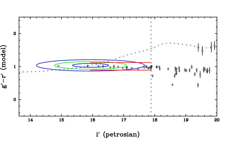
Figure 1: Color magnitude diagram for galaxies near a SDSS cluster at redshift z=0.15. The dotted curve running from lower left to upper right is the mean BCG color-magnitude relation as a function of increasing redshift. Ellipses represent the 1-, 2- and 3-$\sigma$ contours around the mean BCG color and magnitude relation (determined from known BCG’s measured in SDSS data), evaluated at the best-fit redshift. The vertical dotted line represents the 14 cutoff at 0.5$L_{*}$ in $i^{\prime}$ at the redshift of the cluster. Galaxies in the ridgeline (defined by the 0.5$L_{*}$ line and the 2 horizontal lines running from $i^{\prime}$= 16 to 18) and within 0.667 Mpc of the BCG are counted as in the cluster. The number of cluster members combined with a fit to the BCG color-magnitude relation are used to estimate the likelihood of the cluster identification.

The MaxBCG cluster identification algorithm (Annis et al., 2001) relies on the fact that brightest cluster galaxies (BCGs) form a narrowly defined class; they have a small dispersion in luminosity and an even tighter relation in color (see also Gladders & Yee (2000)). For each SDSS galaxy we calculate a “BCG likelihood” based on its color and magnitude. We combine this BCG likelihood with the number of neighboring galaxies found in the corresponding E/SO ridge line to define a cluster likelihood. This likelihood is calculated for every redshift from 0.0 to 0.6 at intervals of 0.01. The redshift is chosen to maximize the cluster likelihood. Elliptical galaxies, which have very regular colors, provide excellent photometric redshift targets. Since each cluster includes a number of these galaxies, photometric redshift estimates for these clusters are excellent. The dispersion between 2406 estimated BCG redshifts and their SDSS spectroscopic redshifts is $\Delta z$ = 0.018. Figure 1 shows a schematic of the technique.

2.3 X–ray Matches

The X–ray data are taken from the ROSAT All-Sky Survey (Trümper, 1983; Voges et al., 1999). The combined RASS bright and faint source catalogs (Voges et al., 1999, 2000) are correlated with the MaxBCG sources discussed above to find X–ray emitting SDSS/RASS clusters (SRC). Matches were found based on a search radius of 80^′′ which corresponds to a net purity of 75% based on comparison with random associations (see Figure 2). Initial optical selection allows us to identify X–ray emitting clusters at fluxes substantially below the flux limits of X–ray selected cluster surveys. This sample was then visually inspected and potentially contaminated cluster matches were excluded for the analysis discussed in this paper. This process yielded a conservative sample of 50 SRC clusters.

As the X–ray count rate for extended sources like clusters of galaxies in the RASS is not very accurate, we used both the Growth Curve Analysis of Böhringer et al. (2000) and an independent analysis to compute the count rates of these clusters. Both techniques agree within the uncertainties. These count rates are converted to bolometric X–ray luminosities using the photometric redshift, a luminosity–temperature relationship, and the ROSAT response matrix. Details are reported in Voges et al. (2001).

3 Lensing Analysis

Foreground mass distributions induce coherent distortions in the images of background galaxies. On average, background galaxies appear tangentially aligned with respect to the foreground lens. The tangential shear, $\gamma_{+}$, is related to the projected mass distribution of the foreground lens, $\Sigma$, by

$$\gamma_{+}(R)=\overline{\kappa}(\leq R)-\overline{\kappa}(R),$$ (3)

where $\kappa=\Sigma/\Sigma_{crit}$ is the surface density normalized by $\Sigma_{crit}$, the critical density for multiple lensing (Miralda-Escudé, 1991). The first term on the right hand side of equation 3 is the mean scaled density interior to projected radius $R$ and the second is the mean scaled density at $R$. The critical density depends only on the geometry of the source-lens-observer system:

$$\Sigma_{crit}={c^{2}\over{4\pi G}}{D_{S}\over{D_{L}D_{LS}}},$$ (4)

where $D_{S}$ and $D_{L}$ are the angular diameter distances from observer to to source and lens, respectively, and $D_{LS}$ is the angular diameter distance from lens to source.

Assuming that the orientations of unlensed background galaxies are uncorrelated with the position of a foreground mass, the shear can be estimated directly from the shapes of background galaxies. It can be shown that the shear induced by weak lensing ($\kappa<<1$) is simply equal to half the induced ellipticity as measured in the tangential frame (Miralda-Escudé, 1991). We denote the tangential component of the ellipticity as $e_{+}$, and the orthogonal component as $e_{\times}$. Note the ellipticity parameter transforms as 2$\theta$ under rotations, so the “orthogonal” frame is rotated by 45$\arcdeg$ with respect to the tangential.

Galaxies are intrinsically elliptical, so the shear measurement must be done statistically by averaging the shapes of many source galaxies:

$$\hat{\gamma}_{+}={1\over{2S_{Sh}}}\langle e^{i}_{+}\rangle={1\over{2S_{Sh}}}{{\sum{w_{i}e^{i}_{+}}\over{\sum{w_{i}}}}},$$ (5)

where $S_{Sh}\sim 0.88$ is the average responsivity of the source galaxies to a shear as defined in F00, and is similar to the shear polarizability defined in Kaiser et al. (1995). The $w_{i}$ are the weights for each shape measurement.

There are two dominant sources of random noise in shear measurements: the intrinsic variance in galaxy shape, or “shape noise” $\sigma_{SN}=\langle e_{i}^{2}\rangle\sim 0.32$, and the uncertainty in the shape measurement of each galaxy $\sigma_{i}\sim 0.25$. For optimal S/N we weight by $1/N^{2}$, $w_{i}=1/(\sigma_{i}^{2}.+\sigma_{SN}^{2})$.

Because SDSS images are relatively shallow, the number density of source galaxies behind each lens is low, about 2 per square arcminute. For this cluster sample, the typical mean induced ellipticity within 600^′′ is $2\gamma_{+}<0.01$. Thus our sensitivity, $\sim 0.4/\sqrt{N_{Source}}$, is insufficient to detect the shear induced by a single lens with precision. To improve the S/N, we average the shear from many lenses.

Averaging over many lenses increases the signal to noise of the shear measurement. Each lens has a different lensing strength, however, which scales as $\Sigma_{crit}^{-1}$. This means lenses with the same mass but different redshifts will not produce the same shear. We rescale the shear to a density contrast, which is a redshift independent quantity, by multiplying both sides of equation 3 by $\Sigma_{crit}$:

$$\Delta\Sigma\ \tbond\ \overline{\Sigma}(\leq R)-\Sigma(R)=\gamma_{+}\Sigma_{crit}.$$ (6)

The weight for each measurement, $w_{i}$, must also be rescaled to $W_{i}=w_{i}\Sigma_{crit}^{-2}$.

The total weight for a given cluster is $\sim N_{source}/\Sigma_{crit}^{2}$, assuming that the measurement error is approximately the same for each source. Because the lensing signal is proportional to $1/\Sigma_{crit}$, this is equivalent to weighting by the relative $\left(S/N\right)^{2}$. Nearby clusters will have larger $N_{source}$, whereas clusters at $z\sim 0.15$ will have large lensing strength $1/\Sigma_{crit}$ (see figure 3(b)). The combination of these two effects conspires to give clusters at $z\sim 0.09$ the largest relative weight.

To find the average density contrast, we need to determine $\Sigma_{crit}^{-1}$, the lensing strength of each lens-source pair, which depends on the redshift of both lens and source. We have a good photometric redshift for each cluster, but we do not have a redshift for each source galaxy. As a result, we estimate the average lensing strength of each cluster by integrating over the source redshift distribution:

$$\Sigma_{crit}^{-1}(z_{L})={{\int_{z_{L}}^{\infty}\Sigma_{crit}^{-1}(z_{L},z_{s})P(z_{s})dz_{s}}},$$ (7)

where P($z_{s}$) is the normalized source redshift distribution. The fact that some source galaxies are in front of the lens, and dilute the signal, is accounted for by beginning the integral at $z_{L}$.

To estimate the redshift distribution in equation 7 we first gather a sample of galaxies with known redshifts drawn from the SDSS and the Canada-France Redshift Survey (CFRS: Lilly et al. (1995)). CFRS galaxies have magnitudes measured in V and I. We convert these to $r^{\prime}$ using the relation $r^{\prime}=I_{CFRS}+0.5(V_{CFRS}-I_{CFRS})$. This relation is empirically determined from galaxies observed by both SDSS and CFRS.

The redshift distributions of these galaxies, in bins of $r^{\prime}$, are fit to the function (Baugh & Efstathiou (1993))

$$n(z)\varpropto z^{2}exp(-({{z}/{z_{c}}})^{3/2}).$$ (8)

The values of $z_{c}$ are then used to derive a relationship between $r^{\prime}$ and $z_{c}$. The derived $z_{c}$ vs. $r^{\prime}$ relation has been independently confirmed by comparison of SDSS and CNOCII data (Yee et al., 2000).

For the lensing measurements, we choose “background,” or source galaxies with reddening corrected Petrosian magnitude 18.0 $<$ $r^{\prime}$$<$ 22.0 and size 4$\sigma$ larger than the stellar locus (see F00). We have source galaxy catalogs with measured shapes in $g^{\prime}$, $r^{\prime}$, and $i^{\prime}$ bands, containing 1.7, 2.4, and 2.1 million objects respectively. The magnitude distribution of each catalog is converted to a redshift distribution using the derived $r^{\prime}$-$z_{c}$ relationship. The inferred redshift distribution for each of these catalogs is shown in Fig. 3(a), and 3(b) shows the lensing strength $\Sigma_{crit}^{-1}(z_{L})$ derived from the redshift distributions.

Some source galaxies are in front of the lens, and this is accounted for in equation 7, but a few galaxies in our source catalog are physically associated with the clusters. The number density of these galaxies will decrease with physical radius from the center of the cluster and their inclusion in the analysis will radially bias the shear estimate. To correct for this effect, we compare the number of background galaxies around random points to those around

lenses. We choose 100 random points for each lens, and assume an excess of background galaxies is due to objects physically associated with the lens. We correct for this dilution by multiplying the measured shear by a radial correction factor F(r) = $\langle N_{lens}\rangle/\langle N_{rand}\rangle$, the ratio of source galaxies around lenses to that around random points. The average correction factor ranges from a factor of 1.5 in the innermost bin to 1.02 in the outermost (see §4.1).

It should be noted that the magnification of background sources by the foreground lens may also increase the number density of neighboring galaxies. The magnification will bring faint galaxies into our magnitude limited catalog. On the other hand, the geometric distortion introduced by the lens moves background galaxies apart, diluting the number density of sources. The relative change in the number density goes as $N^{\prime}/N_{0}\varpropto\mu^{2.5s-1}$, where $\mu=1+\epsilon$ is the magnification and s is the slope of the galaxy number counts (Broadhurste, Taylor, and Peacock, 1995). For these clusters, $\epsilon\sim$ shear $\lesssim.01$. Thus, for s on the order of 0.4, which it is for our background galaxies, the effect of magnification is small compared to the neighbor excess which is $\lesssim 0.5$.

4 Results

We begin with 50 clusters found in the SDSS imaging data and matched to RASS as described in §2.3. We then choose clusters with redshift $z<0.4$. The upper limit of z=0.4 is where photometric redshift estimation becomes less accurate as the 4000Å  break passes between the $g^{\prime}$ and $r^{\prime}$ bandpasses. To ensure that residual systematic shape correlations do not bias the shear estimate, we demand that the azimuthal distribution of source galaxies around each lens be reasonably symmetric. After these cuts we are left with 42 clusters, with a photometric redshift distribution is shown in Figure 4. Their ROSAT bolometric X–ray luminosities range from 8.5$\times 10^{41}$ to 4.4$\times 10^{44}$ ergs/s, with a distribution of X–ray luminosities as shown in Figure 5

4.1 Cluster Density Profile

The shear in the annulus 20-2000 kpc, centered on the BCG, is $(3.3\pm 0.5)\times 10^{-3}$, which is a detection at the $\sim$7-$\sigma$ level (see Table 1). Because the shear is a redshift dependent quantity, we rescale each shear measurement to a density contrast as discussed in §3. Fig. 6 shows the average density contrast measured in nine radial bins centered on the BCG. The independent radial bins have centers ranging from 150 to 1890 $h^{-1}$ kpc. We have applied a correction factor for contamination by cluster members as described in §3 For this figure we have combined the measurements made in the $g^{\prime}$, $r^{\prime}$, and $i^{\prime}$ bandpasses.

As a test to see if our signal is due to gravitational lensing, we have measured the orthogonal component of the shear, $\gamma_{\times}=\langle e_{\times}\rangle/2$ in the same radial bins used for measurement of the tangential shear. This measurement is equivalent to measuring the curl of the gradient of $\kappa$ and should be zero (Kaiser, 1995; Stebbins, Mckay, & Frieman, 1996). We find that the $\gamma_{\times}$ profile is indeed a good fit to zero ($\chi^{2}$ = 7.0/9). We have also run tests for systematics in the background galaxy shapes and bias in the shear measurement due to the faint tails of foreground galaxy light distributions. Both of these tests are null and details can be found in F00.

We fit the observed density contrast in $g^{\prime}$, $r^{\prime}$, and $i^{\prime}$ to a power law of the form $\Delta\Sigma(R)\varpropto R^{\gamma}$, using the full covariance matrix to estimate the chi squared statistic. We find $\gamma=-0.9\pm 0.3$. A power law shear profile implies the same power law for the projected mass density profile. Note again that we have used the BCG as the center for our measurements. The use of any position for the center which is not the true center of mass will complicate the interpretation of these fits (see §5).

4.2 Cluster Model

The average cluster density contrast is consistent with that of a projected singular isothermal sphere (SIS); $\gamma=-1$. Cluster density profiles inferred from lensing are typically well fit by an isothermal (Fischer & Tyson, 1997). We will use this model for the remainder of the paper to represent the average cluster density profile. The SIS model has projected density

$$\Sigma(R)=116\left(\sigma_{v}\over 1000\textrm{km/s}\right)^{2}\left(R\over 1\textrm{Mpc}\right)^{-1}\textrm{M${}_{\sun}$ pc${}^{-2}$}.$$ (9)

To estimate masses, we simply fit the measured profile to a 1/R density with one free parameter, the velocity dispersion $\sigma_{v}$. Note that a SIS has a density contrast equal to the density itself, $\Delta\Sigma(R)=\Sigma(R)$.

Once the velocity dispersion is estimated, the density can be integrated to give the total mass within a projected radius $R$. The mass of an SIS within projected radius R is a factor of $\pi/2$ larger than the mass within the three dimensional radius r=R.

4.3 Mass vs. L_X

Table 1 contains fits to equation 9 for the sample as a whole as well as two subsamples, split by their X–ray luminosity. The shear profiles for the subsamples are both consistent with isothermal. The average bolometric L_x is calculated by weighting the individual L_x of each cluster with its relative weight in the shear measurement $\approx N_{source}/\Sigma_{crit}^{2}$.

We use the fits to equation 9 to infer the velocity dispersion and the mass within 1 Mpc. The mass of the higher L_X subsample is substantially higher than the low L_X subsample. Because the clusters are different sizes, it is more meaningful to discuss the mass within a characteristic radius $r_{500}$, the radius within which the mean density falls to 500 times the critical density at that redshift. The fits to $r_{500}$ and the projected mass within $r_{500}$ are also shown in Table 1. Again, the mass of the higher L_X subsample is substantially higher.

5 Systematic Error

Possible sources of systematic error in the mass measurements are errors in the correction for blurring by the PSF and inclusion of stars in the source galaxies. The blurring correction and stellar contamination were addressed in F00, and are less than 10% and 1% respectively. Other possibilities are variations of angular diameter distance with cosmological model, unertainties in the source galaxy redshift distribution, and offsets of the BCG from the true center of mass of the cluster.

Lensing masses were calculated in 3 different cosmologies: $\left(\Omega_{M},\Omega_{\Lambda}\right)$ = $\left(1.0,0.0\right)$, $\left(0.3,0.0\right)$, $\left(0.3,0.7\right)$. We find that the mass estimates vary by less than 5% between these cosmologies.

The procedure for estimating the redshift distribution is based on the $r^{\prime}$ magnitude distribution of the sources (see §3). In order to understand the uncertainty in the derived distribution, we examined the range of allowed $z_{c}$ values in the fit to Eq. 8. Using the 68% confidence limits from our $\chi^{2}$ fits, we find that the derived masses vary by less than 5%.

Differences in selection criteria between galaxies in CFRS and SDSS might also bias the assumed source redshift distribution. We intend to address this limitation in the future by directly obtaining redshifts for a sub-sample of the source galaxy catalog.

In this paper we have used the BCG as the center for our lensing measurements. As we have stated above, the use of any center other than the true center of mass may bias the mass estimates. An alternative is to use the RASS position, but these are ill-determined for these low-flux, extended sources (Voges et al., 2000). The mean offset between BCG and measured X–ray centroid is 85kpc (max $\sim$200kpc). However, because we use apertures much greater than 85kpc, we do not expect our mass measurements to differ significantly for these centroid shifts. We have repeated our analysis using the X–ray centroid as the center and the signal remained within the 1-$\sigma$ error limits.

We have further checked our sensitivity to offsets by repeating the analysis with centers artificially offset from the BCG by various amounts and in random directions. Figure 7 shows the $i^{\prime}$-band shear in a 1.1Mpc aperture measured as a function of artificial centroid shift. The shear is not changed substantially for shifts less than about 200kpc. Our mass estimates are also unchanged for shifts less than 200kpc. Furthermore, the shear becomes consistent with zero for shifts that approach the size of the aperture. Because we do not know the true mass distribution of these objects, we cannot measure the offsets with this data alone. However, this test is consistent with the assumption that the true center is within the aperture and is less than 200kpc from the BCG. Until we can find the true center of mass, or at least estimate the mean size of the offsets, we will not be able to quantitatively determine the effect of these offsets on our mass estimates. This issue will be dealt with in a future paper.

An issue related to centroid offsets is the problem of sub-structure within clusters. If there are substantial sub-clumps in a cluster, not only is the BCG unlikely to be at the centroid, but the density profile will not be isothermal. In particular, the slope of the shear profile at large radii will become flatter than expected from an isothermal, as sub-clumps become included within the aperture (Clowe, Luppino, Kaiser, & Gioia, 2000). This will make an SIS model an inappropriate representation of the data. However, the reduced $\chi^{2}$ for the SIS fits to 42 clusters is 3.3/8=0.4, suggesting that, in the ensemble average, sub-clumping is not a dominant source of error.

6 Conclusions

We have demonstrated the ability to measure ensemble cluster masses using SDSS imaging data. We detect the shear from 42 SRC clusters with high signal to noise, and find a correlation between the derived lensing mass and X–ray luminosity. The current sample represents only 4% of the final SDSS data set. Extrapolating, we expect $\gtrsim$ 1000 MaxBCG/RASS clusters, and perhaps more with the addition of the catalogs of Kim et al. (2000) and Nichol et al. (2000). With the final sample, we will be able to measure the M-L_X relation with high precision. The excellent 5-band photometry of the SDSS will yield measurements of the total light in each cluster. Furthermore, SDSS spectroscopy of the nearby clusters will yield an estimate their velocity dispersion. Thus in addition to the L_X-M, we will measure scaling relations between lensing mass, visible light in 5 bandpasses, and velocity dispersion, all measured from SDSS data. These scaling relations will greatly enhance our understanding of cluster physics.

Scaling relations for other classes of objects can be studied in a similar fashion. Though individual galaxies and groups are much less massive than clusters, and hence are less effective lenses, they are far more common. As a result, our sensitivity to ensemble masses of galaxies (F00), groups, and clusters are similar. This new ability to measure ensemble masses for classes of objects should contribute substantially to our understanding of the relationship between mass and luminous matter in the universe.

Figure 2: Angular separations between optically selected cluster candidates and RASS bright and faint source catalog objects. The diamonds are the number of matches between the MaxBCG objects and RASS. Error bars are $\pm 1\sigma$ Poisson. The solid line is the mean number of matches to 100 sets of random points, each set containing the same number of points as the MaxBCG. The ratio of the cluster matches to the random matches is the purity of the sample at a given radius. The total purity within 80^′′ is $\sim$ 75%.

Figure 3: (a) Redshift distributions for source galaxies found in $g^{\prime}$(dashed line), $r^{\prime}$(solid), and $i^{\prime}$(dot-dashed) inferred from their $r^{\prime}$magnitudes. (b) The lensing strength, $\Sigma_{crit}^{-1}$, vs. lens redshift, calculated from the redshift distributions shown in (a).

Figure 4: Photometric redshift distribution for the 42 SRC clusters used in the lensing analysis.

Figure 5: Distribution of bolometric X–ray luminosities for the 42 SRC clusters used in the lensing analysis.

Figure 6: Average projected density contrast for 42 SRC clusters. For this plot we have combined the measurements made in the $g^{\prime}$, $r^{\prime}$, and $i^{\prime}$ bandpasses. The solid line is the best fitting power law, $\Delta\Sigma\varpropto R^{-0.9}$. Errors bars are $\pm 1\sigma$.

Figure 7: Shear within a 1.1Mpc aperture measured as a function of artificial offset from the BCG. Shear is measured in the $i^{\prime}$ band. The shear is not changed substantially for offsets less than 200kpc. The shear becomes consistent with zero as the offset approaches the size of the aperture.

Table 1: Fits to Singular Isothermal Spheres

$\langle L_{X}^{bol}\rangle$	NClust	$\langle\gamma_{T}(20-2000$kpc$)\rangle$	$\sigma_{v}$	M($<1h^{-1}$Mpc)	$r_{500}$	M($<$ $r_{500}$ )
($\times 10^{44}h^{-2}$ ergs/s)		$(\times 10^{-3})$	(km/s)	($\times 10^{14}h^{-1}$M☉)	($h^{-1}$Mpc)	($\times 10^{14}h^{-1}$M☉)
0.30 $\pm$ 0.06	42	3.3$\pm$0.5	530${}^{+40}_{-50}$	2.1${}^{+0.3}_{-0.4}$	0.41	0.9 $\pm$ 0.2
0.14 $\pm$ 0.03	27	2.2$\pm$0.5	490 $\pm$ 60	1.8 $\pm$ 0.4	0.39	0.7 $\pm$ 0.2
1.0 $\pm$ 0.09	15	9.0$\pm$1.5	800${}^{+90}_{-110}$	4.7${}^{+1.0}_{-1.3}$	0.57	2.7${}^{+0.9}_{-1.1}$

Note. — The first row is the average over the entire sample of clusters and the subsequent rows are subsamples. All masses are projected values.

References

- Annis et al. (2001) Annis, J., et al. 2001 in preparation
- Bernstein et al. (2001) Bernstein, G. M., Jarvis, R. M., Fischer, P., & Smith, D. R. 2001 in preparation
- Baugh & Efstathiou (1993) Baugh, C. M. and Efstathiou, G. 1993, MNRAS, 265, 145
- Broadhurste, Taylor, and Peacock (1995) Broadhurst, T.J., Taylor, A. N., Peacock, J.A., 1995, ApJ, 438, 49
- Clowe, Luppino, Kaiser, & Gioia (2000) Clowe, D., Luppino, G.A., Kaiser, N., Gioia, I.M. 2000, ApJ, 539, 540
- Böhringer et al. (2000) Böhringer, et al. 2000, submitted to A&A, in press (astro-ph/0003219)
- Fischer & Tyson (1997) Fischer, P & Tyson, J. A. 1997, AJ, 114 14
- Fischer et al. (2000) Fischer, et al. 2000, AJ, 120, 1198, (F00)
- Fukugita et al. (1996) Fukugita, M., Ichikawa, T., Gunn, J. E., Doi, M., Shimasaku, K., & Schneider, D. P. 1996, AJ, 111, 1748
- Gladders & Yee (2000) Gladders, M. D., Yee, H. K. C., 2000, AJ, 120, 2148
- Gunn et al. (1998) Gunn, J. E., et al. 1998, AJ, 116, 3040
- Joffre et al. (2000) Joffre, M., et al. 2000, ApJ, 534, L131
- Kaiser et al. (1995) Kaiser, N., Squires, G. & Broadhurst, T. 1995, ApJ, 449, 460
- Kaiser (1995) Kaiser, N., ApJ, 439, L1
- Kim et al. (2000) Kim, R., et al. 2001, in preparation.
- Lilly et al. (1995) Lilly, S., J., et al. 1995, ApJ, 455, 50
- Lupton et al. (2000) Lupton, R. H. et al. 2000, in preparation for publication in AJ
- Miralda-Escudé (1991) Miralda-Escudé, J. 1991, ApJ, 370, 1
- Nichol et al. (2000) Nichol, B., et al. 2001, in preparation
- Squires et al. (1996) Squires, G., Kaiser, N., Babul, A., Fahlman, G., Woods, D., Neumann, D. M., Böhringer, H. 1996, ApJ, 461, 572
- Smail et al. (1997) Smail, I. et al. 1997, ApJ, 479, 70
- Stebbins, Mckay, & Frieman (1996) Stebbins, A., Mckay, T., & Frieman, J. 1996, in “IAU 173: Astrophysical Applications of Gravitational Lensing,” eds. C. S. Kochanek & J. N. Hewitt, (Kluwer), p. 75
- Trümper (1983) Trümper, J., 1983, Adv. Space Res. 27, 1404
- Voges et al. (1999) Voges, W., et al., 1999, A & A, 349, 389
- Voges et al. (2000) Voges, W., et al., 2000, IAUC 7432
- Voges et al. (2001) Voges, W., et al. 2001, in preparation
- Yee et al. (2000) Yee, H., et al. 2000, ApJS, 129, 475
- York et al. (2000) York, D. G. et al. 2000, AJ, 120, 1579