Possible Detection of Baryonic Fluctuations in the Large-Scale Structure Power Spectrum

Abstract

We present a joint analysis of the power spectra of density fluctuations from three independent cosmological redshift surveys; the PSCz galaxy catalog, the APM galaxy cluster catalog and the Abell/ACO cluster catalog. Over the range $0.03\leq k\leq 0.15h$Mpc^-1, the amplitudes of these three power spectra are related through a simple linear biasing model with $b=1.5$ and $b=3.6$ for Abell/ACO versus APM and Abell/ACO versus the PSCz respectively. Furthermore, the shape of these power spectra are remarkably similar despite the fact that they are comprised of significantly different objects (individual galaxies through to rich clusters). Individually, each of these surveys show visible evidence for “valleys” in their power spectra – i.e. departures from a smooth featureless spectrum – at similar wavenumbers. We use a newly developed statistical technique called the False Discovery Rate, to show that these “valleys” are statistically significant. One favored cosmological explanation for such features in the power spectrum is the presence of a non-negligible baryon fraction ($\Omega_{b}$) in the Universe which causes acoustic oscillations in the transfer function of adiabatic inflationary models. We have performed a maximum-likelihood marginalization over four important cosmological parameters of this model ($\Omega_{m}$, $\Omega_{b}$, $n_{s}$, $H_{o}$). We use a prior on $H_{0}=69\pm{15}$, and find $\Omega_{m}h^{2}=0.12^{+0.03}_{-0.02}$, $\Omega_{b}h^{2}=0.029^{+0.011}_{-0.015}$, $n_{s}=1.08^{+0.17}_{-0.20}$ (2$\sigma$ confidence limits) which are fully consistent with the favored values of these cosmological parameters from the recent Cosmic Microwave Background (CMB) experiments. This agreement strongly suggests that we have detected baryonic oscillations in the power spectrum of matter at a level expected from a Cold Dark Matter (CDM) model normalized to fit these CMB measurements.

1 Introduction

We present a new analysis on the power spectra of density fluctuations ($P(k)$) as derived from three recently available independent cosmological redshift surveys; the Abell/ACO Cluster Survey as defined in Miller & Batuski (2001) and Miller et al. (2001a), the IRAS Point Source redshift catalog (PSCz; Saunders et al. 2000), and the Automated Plate Machine (APM) cluster catalog (Dalton et al. 1994). For the first time, the volumes traced by these surveys are large enough to accurately probe the power spectrum to wavenumbers of $k=0.015$ (Abell/ACO), $0.025$ (PSCz) and $0.030h$Mpc^-1 (APM). Throughout, we use $h=H_{o}/100$km s^-1Mpc^-1.

Such information on the large–scale distribution of matter in the Universe is critical for constraining cosmological models of structure formation as well as determining the cosmological parameters. For example, the amplitude and shape of $P(k)$ below $k\sim 0.05h$Mpc^-1 can be used to discriminate between a high and low value of $\Omega_{m}h$, while a non-negligible baryon fraction ($\Omega_{b}$) would produce noticeable oscillations in $P(k)$ at $k<0.1h$Mpc^-1 (with the oscillations becoming broader, and more easily detectable, toward smaller $k$; see Eisenstein et al. 1998). Cosmological constraints based on the large–scale structure (LSS) in the Universe are independent and complementary to those derived from the Type Ia supernovae and Cosmic Microwave Background (CMB) experiments (see Bond et al. 2000; Jaffe et al. 2000) and thus breaking key degeneracies inherent in these other cosmological measurements (see, for example, Tegmark, Zaldarriaga & Hamilton 2001).

In the past, cosmological studies of the power spectrum of density fluctuations have been hampered in three ways; i) uncertainties in the shape of the $P(k)$ on very large scales, ii) the form of the relative biasing between the luminous and dark matter, and iii) the possible existence of a narrow “bump” in the $P(k)$ (Landy et al. 1996; Einasto et al. 1997). As we will show in Sections 2 and 3, our new data-sets allow us to address these concerns and thus facilitate a more robust determination of the cosmological parameters from LSS measurements. Our work differs from other recent attempts to constrain cosmological models using LSS data (Novosyadlyj et al. 2000; Tegmark et al. 2001; Efstathiou & Moody 2000; Huterer, Knox & Nichol 2000) since we first focus on the detection and interpretation of features in the matter power spectrum, followed by parameter estimation based on the favored models that explain these features.

2 Biasing

In Figure 1 (top) we plot the $P(k)$ for our three samples. The Abell/ACO power spectrum is from Miller & Batuski (2001), the APM result is from Tadros, Efstathiou, and Dalton (1998), and the PSCz data are from Hamilton & Tegmark (2000). In all three plots, we exclude any data with errors $>50$% of the power for obvious reasons but we note that their inclusion makes no differences in our final results. The errors are all $1\sigma$ as quoted by the authors. In the bottom frame, we plot the same data for the three samples after shifting the amplitudes of the APM and PSCz surveys to match that of the Abell/ACO survey. We have applied various techniques to calculate this amplitude shift (e.g. a $\chi^{2}$ minimization of the data with nearly identical $k$-values as well as using model fits to the data and re–normalizing them to the Abell/ACO data), but in all cases we obtain nearly identical results: the relative bias between the three samples over the range $0.03\leq k\leq 0.15h$Mpc^-1 is $b=1.5$ and $b=3.6$ for Abell/ACO versus APM and Abell/ACO versus the PSCz respectively.

A remarkable aspect of Figure 1 is the overall success of a simple linear biasing model in re-normalizing the amplitudes of these power spectra over nearly a decade of scale. A scale–independent biasing model, over the scales discussed herein, has already been predicted from recent numerical simulations (Narayanan, Berlind & Weinberg 2000) and therefore, allows us to confidently re-scale these three different power spectra, thus facilitating the detection of features in the combined $P(k)$ as discussed below.

3 The Shape of the Power Spectrum

The overall shape of our combined power spectrum is shown in Figure 1 and it is unique for two reasons. First, we see no evidence at small $k$ values for a turn–over in the $P(k)$ toward a scale-invariant spectrum as previously hinted at in other LSS analyses (Tadros & Efstathiou 1996; Peacock 1997; Gatzañaga & Baugh 1998). This large-scale power has also been witnessed in other recently reported $P(k)$ measurements (see Efstathiou & Moody 2000; Schuecker et al. 2001). Such large–scale power in the $P(k)$ indicates a low value for the shape parameter ($\Gamma=\Omega_{m}\,h<0.3$) since this has the effect of sliding the matter power spectrum to the smaller $k$ values compared to a critical matter density universe. Secondly, we do not find a narrow “bump” in the $P(k)$ as reported by Einasto et al. (1997) and Landy et al. (1996) but instead witness “valleys” in the power spectrum. However, these previous surveys did not have the volume to see the large scale ($k<0.03$) power in $P(k)$ and thus only saw the down–turn of the “valley” giving the appearance of a “bump” in the power spectrum at $k\simeq 0.05$ and therefore, our $P(k)$ may still be consistent with the Landy et al. and the Einasto et al. power spectra. For the remainder of this section, we focus on the the two “valleys” we see in Figure 1 at $k\simeq 0.035$ and $k\simeq 0.090h$Mpc^-1.

3.1 False Discovery Rate

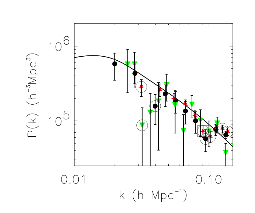
Figure 2: Here, we show the amplitude shifted power spectra for the three samples of uncorrelated data. The points highlighted with a circle denote rejections with $\alpha=0.25$ (e.g. a quarter of the rejections may be mistakes). The points highlighted by squares are for $\alpha=0.10$ (e.g. a tenth of the rejections may be mistakes). The analysis utilizes our best-fit model with the baryon wiggles removed as the null hypothesis. By controlling the false discovery rate, we can say with statistical confidence that the two “valleys” are detected as features in the power spectra.

In this section, we investigate the statistical significance of the two features seen in Figures 1 and 2. We wish to determine if all of the data points are consistent with being drawn from a smooth, featureless, power spectrum. In the statistical literature, this is known as multiple hypothesis testing since one is testing, for each point, the null hypothesis that it was drawn from a featureless $P(k)$. The key issue then becomes choosing the threshold (in probability) which these null hypotheses are rejected.

Traditionally, this is done by rejecting all points that are above a certain $\sigma_{rej}$ threshold. Unfortunately, there is a major problem with this methodology since the number of data points that are mistakenly rejected depends on the size of the data-set. For example, if all our 37 data points were uncorrelated and truly drawn from a smooth $P(k)$, we would expect, on average, only 1.75 of these data points to be rejected (and thus in error) for a $\sigma_{rej}=2$ threshold. However, if we had one million data points, then the number mistakenly rejected data points at the $\sigma_{rej}=2$ level would be approximately 50,000. [Note: this comparison only works if all of the real data were uncorrelated.] To guard against the over-detection of false discoveries, one could arbitrarily increase the significance threshold to $\sigma_{rej}=4$, thus reducing the number of errors but would lead to a much more conservative test. This is not to say that all of the $2\sigma$ rejections would be wrong, but simply that you would have many more false rejections. Thus, any significance threshold is arbitrary and highly dependent on the data size. So, enforcing a $\sigma_{rej}=3$ threshold for small data-sets can be overly conservative. In summary, the more tests one does, the more stringent the required threshold becomes to avoid making too many false discoveries.

Ideally, we need a statistical technique that is more adaptive and whose interpretation does not depend on the data size. Instead of $\sigma_{rej}$, we will choose to control the false discovery rate ($\alpha$)– which is defined to be the percentage of mistakenly rejected points out of the total number of points rejected. This is clearly independent of the data size. Such an adaptive statistical tool is the False Discovery Rate (FDR; Benjamini & Hochberg 1995). Once we choose $\alpha$, then FDR defines an appropriate significance threshold to obtain this false discovery rate for the dataset in question. For example, if we choose $\alpha=\frac{1}{4}$ and reject eight data points, then on average, only two of these points are in error even though their significance (as implied by their $\sigma$’s) may appear low. Again, arbitrarily setting $\sigma_{rej}=3$ for our data-set may be too conservative. Instead, by a priori controlling the false discovery rate, we can state with statistical confidence that six out of eight rejected data points are true outliers against the null hypothesis. We briefly discuss FDR here and refer the reader to Nichol et al. 2000 and Miller et al. 2001b for further details.

Operationally, we first compute the $p$–value for each test. Herein we have used a a smooth CDM model based on our best-fit cosmological parameters (Section 4) but with the baryon oscillations removed (see Eisenstein & Hu 1998). However, the reader should note that this model is nearly an exact power-law over the range $k>0.02h$Mpc^-1, and so our results would not change if we used a simple power-law fit to the data (without the valleys). We then rank, in increasing size, the $p$-values (for each test) and draw a line of slope $\alpha$ and zero intercept. Recall, $\alpha$ is the maximum acceptable false discovery rate. The first crossing of this line with a $p$–value (moving from larger to smaller $p$–values) defines the significance threshold $\sigma_{rej}$, below which all points are rejected based on our null hypotheses. On average, only $\alpha\times 100\%$ of these rejected points will be in error.

Figure 2 presents the result of applying FDR to our combined $P(k)$ using an uncorrelated dataset (as opposed to the correlated data in Figure 1). Specifically, we use the uncorrelated $P(k)$ given by Tegmark & Hamilton (2000) for the PSCz while Tadros et al. (1998) claim their APM $P(k)$ is uncorrelated and thus we use their data points directly. For the Abell/ACO catalog, Miller & Batuski (2001) have shown that their $P(k)$ is uncorrelated for separations of $\Delta k\simeq 0.015h$Mpc^-1. Therefore, as can be seen from Figure 1, the data at $k>0.04$ is already uncorrelated while for smaller $k$ values we simply re–sample the data in such a way that the minimum separation between points is at least $\Delta k\sim 0.01h$Mpc^-1. In Figure 2, the circled points are rejected (based on our null hypotheses) with a false discovery rate of $\alpha=0.25$, while the points outlined with squares are rejected with a $\alpha=0.10$.

We detect the “valleys” at both $k\sim 0.035h$Mpc^-1 and at $k\sim 0.09h$Mpc^-1. The power of the false discovery rate is that it ensures that no more than $25\%$ of the eight rejections (circles) could be incorrect. If we apply the much more stringent constraint of $\alpha=0.1$, we only reject only one point (at $k\sim 0.09h$Mpc^-1), but FDR limits the number of false rejections in this case essentially to zero. This allows us to state with statistical confidence that the fluctuations are true outliers against a smooth, featureless spectrum. Note that each of the three data sets contributes to the features, and so the detection is not dominated by one sample. In the next two sections, we review possible explanations for these observed features in our $P(k)$ including systematic uncertainties and cosmological effects.

3.2 Systematic Uncertainties

In this section, we consider both measurement error and sampling effects as possible explanations for the features seen in the power spectra shown in Figures 1 & 2. To address the first of these, we simply note that Miller & Batuski (2001) used several different methods of calculating the $P(k)$ for the Abell/ACO catalog and observed no significant differences in the measured $P(k)$ for $k\leq 0.02h$Mpc^-1. Further evidence that the fluctuations seen in Figures 1 & 2 are not the result of the methodology comes from the fact that the authors of the three power spectra all used different methodologies to calculate their $P(k)$; the APM survey was analyzed using the method of Feldman et al. (1994), the analysis of the Abell/ACO catalog followed Vogeley et al. (1992) and Feldman et al. (1994), while the PSCz $P(k)$ was derived from a Karhunen - Loeve (KL) eigenmode analysis.

Next, we consider sampling effects e.g. could artifacts of the design and construction of these surveys have produced such features and are the surveys independent and representative of the whole Universe? We believe such effects are highly unlikely for two reasons. First, each of these three surveys was constructed in a different way and thus possess significantly different window functions. For example, the APM survey only covers a steradian of the sky centered on the Southern Galactic Cap, with a near constant number density of clusters/groups over the redshift range $15000\leq cz\leq 35000$km s^-1, while the Abell/ACO cluster sample covers over 2$\pi$ steradian with a near constant number density of rich clusters out to $cz=42000$km s^-1 (in the north) and $cz=30000$km s^-1 (in the south). These two cluster surveys are independent of each other since $\simeq 90\%$ of the APM clusters used by Tadros et al. (1998) are non–Abell systems and are thus not in the Abell/ACO sample (Miller & Batuski 2001). In contrast, the PSCz galaxy redshift survey covers 10.6 steradian (84% of the entire sky) and has a number density that falls off steeply beyond $cz=12000$km s^-1. Therefore, these three surveys sample different volumes of the Universe, use different tracers of the mass (from galaxies through to rich clusters) and are independent of each other.

We stress here that these features are seen in all of the individual power spectra at similar wavenumbers and therefore, not a artifact of combining the three $P(k)$’s, which we did simply to increase the overall statistical significance of these “valleys”. This concordance is a powerful consistency check which argues against statistical and systematic uncertainties producing these features. Moreover, the volume sizes of these three surveys are so large that we hope to have reached a “fair sample” of the Universe and thus these features can not be explained away as unusual and only present in our parts of the Universe. We therefore believe that these fluctuations in the $P(k)$ are physical and in the next section we review possible cosmological explanations for them.

3.3 Cosmological Explanations for the Fluctuations

One possible cosmological explanation for these “valleys” in the observed $P(k)$ is the existence of corresponding features in the initial power spectrum of density fluctuations coming out of Inflation. This explanation has been proposed for the excess power or correlations seen in several of previous surveys (Broadhurst et al. 1990; Landy et al. 1996; Einasto et al. 1997). Unfortunately, the physical mechanism for producing such features in the initial power spectrum remains unclear (see Atrio-Barandela 2000; Einasto 2000).

A more natural and well–understood explanation is the presence of a non-negligible baryon fraction in the Universe which leads to a coupling (at redshifts $z\geq 1000$) between the CMB photons and the baryonic matter thus resulting in acoustic oscillations which leave an imprint on the matter power spectrum (see Eisenstein & Hu 1998 and references therein). Recently, Eisenstein et al. (1998) examined this cosmological model and tested it against three LSS data sets; the APM de–projected $P(k)$ of Gaztañaga & Baugh (1998), the $P(k)$ compilation of Peacock & Dodds (1994), and $P(k)$ from the Abell/ACO sample from Einasto et al. (1997). Only the Einasto et al. $P(k)$ had a noticeable feature (“bump”) in the power spectrum and Eisenstein et al. (1998) were unable to find a satisfactory cosmological model that fitted these data. Their analysis indicated two equally likely fits to the data, one with $\Omega_{m}<0.2$ and the other with $\Omega_{m}>0.7$, while both models needed $\Omega_{b}/\Omega_{m}\simeq 0.3$. The high $\Omega_{m}$ model was excluded by the Big Bang Nucleosynthesis upper limit of $\Omega_{b}h^{2}<0.026$ (Burles, Nollett, and Turner 2000) while the low $\Omega_{m}$ model was rejected by the lack of large–scale power seen in the $P(k)$ for $k<0.05h$Mpc^-1.

We present here new constraints on model $P(k)$ using much improved datasets than those used by Eisenstein et al. (1998). The improvement in the data comes from the larger volumes traced by these surveys, thus allowing smaller $k$’s to be probed with a higher resolution. In the next section, we re-examine this scenario and find that baryonic oscillations match with the power spectra in Figure 1. We note here that Tegmark et al. (2001) also hinted at the possible detection of baryon fluctuations in the PSCz $P(k)$ but a statistical analysis was not performed.

4 Cosmological Parameter Estimation

We have used the cosmological models of Eisenstein & Hu (1998) to perform a parameter estimation which can be compared with the recent CMB results (Tegmark et al. 2001; Jaffe et al. 2000; Bond et al. 2000). We begin by constructing a four-dimensional grid in the parameter space using $\Omega_{m}$, $\Omega_{b}$, $n_{s}$ the spectral index, and the Hubble constant. We apply a weak prior with $H_{0}=69\pm{15}$km s^-1Mpc^-1, which is consistent and more conservative than the final results of the Hubble Space Telescope Key Project (Freedman et al. 2001). We then calculate the maximum likelihood via ${\mathcal{L}}=e^{-\chi^{2}/2}$ where $\chi^{2}$ is calculated using the fitting formulae given in Eisenstein & Hu (1998). In fitting these power spectra, we restrict ourselves to the range of $0.015\,<k\,<0.15$ using the uncorrelated data of Figure 2.

The next issue is to find the global maximum in this multi–dimensional likelihood space. Unfortunately, it is highly possible that this global maximum does not lie on one of our grid points, so to guard against this, we use the simplex method (see Press et al. 1992). We then marginalize over each parameter separately by fixing it to the grid and allowing the other three parameters to vary until we find the corresponding maximum. Our methodology is very similar to that of Tegmark & Zaldarriaga (2000) except for our use of the simplex method to find the maximum likelihood. Tegmark & Zaldarriaga fit a cubic spline to their likelihood grid to find the maxima. However, this function can be ill–behaved if the surface is not smooth (i.e. if $\chi^{2}$ varies rapidly in the region of the minimum which is often the case). Therefore, we advocate the use of the simplex method for future analyses since, in principle, it is less dependent upon the actual likelihood surface. We note that a proper marginalization requires integration over the likelihood function. Tegmark et al. (2001) have shown that this is the same as the maximization technique used herein if the likelihood functions are Gaussian, which appears to be a reasonable approximation for our likelihood functions (see Figure 3).

After marginalizing over the three power spectra separately, we combine the likelihoods together to arrive at our final results. For each of the samples, we allow the amplitude to be a free parameter. In this way, the bias parameter does not explicitly enter into the calculation. In Figure 3, we present the Cash statistic for each marginalized parameter (Cash 1979): ${\rm Cash}_{i}=-2ln\frac{{\mathcal{L}}_{i}}{{\mathcal{L}}_{max}}$, where ${\mathcal{L}}$ is the maximum likelihood determined as a function of the fixed parameter $i$ and allowing the other parameters to vary. ${\mathcal{L}}_{max}$ is the global maximum over all parameter space. If the $log$ likelihood functions can be well-approximated with a second order Taylor expansion, then the Cash statistic becomes analogous to a $\chi^{2}$ distribution. Thus, when we marginalize (i.e. hold one parameter fixed allowing the others to vary), we have one degree-of-freedom and our 95% confidence limits are where our Cash statistic crosses a value of $3.84$. In Table 1, we present our final estimates for the three cosmological parameters, $\Omega_{o},\Omega_{b},$ and $n$. We also list similar recent results from latest CMB data (Tegmark et al. 2001; Jaffe et al. 2000; Novosyadlyj et al. 2000). This table clearly illustrates that our best fit values for these cosmological parameters are fully consistent with these other analyses.

In Figure 4, we present the data in Figure 1 along with our best fit model shown in Table 1. For comparison, we also show two favored zero baryon $n_{s}=1$ models with $\Gamma=0.25$ and $\Gamma=0.14$. Clearly, the baryon model is the best representation given these three possibilities.

Table 1: Parameter Estimation Results

$\Omega_{m}h^{2}$	$\Omega_{b}h^{2}$	$n_{s}$	Confidence	Strong Priors	Data Used	Reference
$0.12^{+0.03}_{-0.02}$	$0.029^{+0.011}_{-0.015}$	$1.08^{+0.17}_{-0.20}$	$2\sigma$		LSS	This Work
$0.22^{+0.07}_{-0.06}$	$0.030^{+0.004}_{-0.004}$	$0.99^{+0.07}_{-0.06}$	$1\sigma$	$\Omega_{tot}=1$	CMB	Jaffe et al. (2000)
$0.16^{+0.02}_{-0.01}$	$0.032^{+0.004}_{-0.004}$	$1.00^{+0.09}_{-0.06}$	$1\sigma$		CMB + LSS	Jaffe et al. (2000)
$0.15^{+}_{-0.15}$	$0.054^{+0.05}_{-0.03}$	$1.43^{+}_{-0.52}$	$2\sigma$		CMB	Tegmark et al. (2001)
$0.23^{+0.16}_{-0.12}$	$0.028^{+0.008}_{-0.009}$	$0.96^{+0.20}_{-0.10}$	$2\sigma$		CMB +LSS	Tegmark et al. (2001)
$0.15^{+0.04}_{-0.02}$	$0.02$	$0.92^{+0.08}_{-0.09}$	$2\sigma$	$\Omega_{b}$ fixed	CMB +LSS	Tegmark et al. (2001)
$0.20^{+0.29}_{-0.11}$	$0.019^{+0.04}_{-0.008}$	$1.12^{+0.27}_{-0.30}$	$1\sigma$	$\Omega_{tot}$ = 1	CMB + LSS + $\sigma_{8}$	Novosyadlyj et al. (2000)
					$Ly-\alpha$ forest + bulk flows

5 Conclusions

We present in this paper new evidence for the detection of statistically significant fluctuations in the matter power spectrum. The most natural explanation for these fluctuations are baryonic oscillations in a Cold Dark Matter universe as outlined in Eisenstein et al. (1998) and Eisenstein & Hu (1998). Using this cosmological model, we have measured $\Omega_{m}$, $\Omega_{b}$, and $n_{s}$, finding values that are fully consistent with those presently favored by the recent CMB experiments (see Table 1). This agreement is primarily due to the extra power seen on large scales (small $k$) as well as the features detected in all three power spectra. In the near future, surveys like the SDSS and 2dF Galaxy Redshift Survey (2dFGRS; Colless et al. 2000) will allow for a more detailed analysis of these baryonic features as well as providing more powerful constraints on the cosmological parameters than those presented here (e.g. Percival et al. 2001). However, we do note that on large scales, the volume sampled by the Abell/ACO catalog discussed herein will remain unrivaled even after the main SDSS and 2dFGRS galaxy redshift surveys are completed and will thus remain, for some time, an important database for studying the large–scale structure in the Universe. However, the SDSS Bright Red Galaxy (BRG; York et al. 2000) redshift survey will supercede all these surveys in terms of volume since it will provide a pseudo–volume–limited sample of galaxies out to $z\simeq 0.45$ carefully selected to sample the power spectrum of mass over as large a range of scales as possible.

Acknowledgments   We are indebted to Chris Genovese and Larry Wasserman for their help with FDR. We thank Christopher Cantaloupo, Adrian Melott, Wayne Hu, Peter Coles, Alex Szalay, Daniel Eisenstein, Andrew Jaffe and John Beacom for helpful advise and suggestions throughout this work.

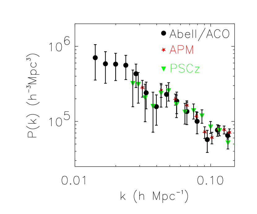
Figure 1: The power spectra for the three samples utilized in this work. The triangles are the PSCz galaxies, the stars are the APM groups and clusters, and the circles are the Abell/ACO rich clusters. The bottom panel shows $P(k)$ after a constant relative bias is applied to the data sets. The shift corresponds to $b=1.5$ and $b=3.6$ for Abell/ACO versus APM and Abell/ACO versus the PSCz respectively.

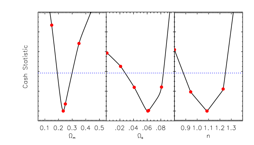
Figure 3: The Cash statistic for the marginalized parameter estimations. The line corresponds to a 95% confidence region.

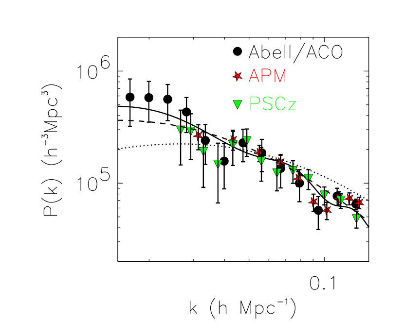
Figure 4: The solid line is the best fit model ($\Omega_{m}=0.24$, $\Omega_{b}=0.061$, and $n_{s}=1.08$ with $H_{0}=69$; see Table 1) plotted with the data from Figure 1 (bottom). The dotted and dashed lines are zero baryon $n_{s}=1$ models with $\Gamma=0.14$ and $\Gamma=0.25$ respectively.

References

- (1) Atrio-Barandela, F., Einasto, J., M ller, V., M cket, J. P., Starobinsky, A. A., 2000, ApJ, submitted (see astro-ph/0012320)
- (2) Benjamini, Y., Hochberg, Y., 1995, J. of the Roy. Soc. Stat. B, 57, 289
- (3) Bond, J. R., et al. see astro-ph/0011378
- Broadhurst, Ellis, Koo & Szalay (1990) Broadhurst, T. J., Ellis, R. S., Koo, D. C. & Szalay, A. S. 1990, Nature, 343, 726
- (5) Burles, S., Nollett, K.M., and Turner, M.S. 2000, preprint astro-ph/0008495
- Cash (1979) Cash, W. 1979, ApJ, 228, 939
- Colless et al. (2000) Colless, M. & 2dF Galaxy Redshift Survey Team 2000, American Astronomical Society Meeting 197, #89.05, 197, 8905
- (8) Dalton, G.B., Croft, R.A.C., Efstathiou, G., Sutherland, W.J., Maddox, S.J., and Davis, M. 1994, MNRAS, 271, 47
- (9) Efstathiou, G., Moody, S.J. 2000, preprint astro-ph/0010478
- (10) Einasto, J., Einasto, M., Gottlöber, S., Müller, V., Saar, V., Starobinsky, A.A., Tago, E., Tucker, D., Andernach, H., & Frisch, P. 1997, Nature, 385, 139
- (11) Einasto, J., 2000, see astro-ph/0011334
- (12) Eisenstein, D.J., Hu, W., Silk, J., and Szalay, A.S. 1998,ApJ, 494, L1
- (13) Eisenstein, D.J., Hu, W. 1998, ApJ, 496, 605
- (14) Feldman, H.A., Kaiser, N., Peacock, J.A. 1994, ApJ, 426, 23
- (15) Freedman et al. 2001, ApJ in press, astro-ph/0012376
- (16) Gatzañaga, E., Baugh, C.M. 1998, MNRAS, 294, 229
- (17) Hamilton, A.J.S., Tegmark, M. 2000, submitted to MNRAS, astro-ph/0008392
- (18) Huterer, D., Knox, L., Nichol, R. C., 2000, ApJ, astro-ph/0011069
- (19) Jaffe et al. 2000, preprint astro-ph/0007333
- (20) Landy, S.D., Shectman, S.A., Lin, H., Kirshner, R.P., Oemler, A.A., Tucker, D. 1996, ApJ, 456, L1
- (21) Miller, C.J., Batuski, D.J. 2001, ApJ, in press
- (22) Miller, C.J., Krughoff, K.S., Batuski, D.J., Slinglend, K.A., Hill, J.M., 2001a, in preparation
- (23) Miller, C.J., Schneider, J., Connolly, A. J., Nichol, R. C., Genovese, C., Moore, A. W., Wasserman, L., 2001b, in preparation
- Narayanan, Berlind & Weinberg (2000) Narayanan, V. K., Berlind, A. A. & Weinberg, D. H. 2000, ApJ, 528, 1
- Nichol et al. (2000) Nichol, R. C., Miller, C. J., Reichart, D., Wasserman, L., Genovese, C., & SDSS Collaboration 2000, American Astronomical Society Meeting 197, #107.03, 197, 110703, see astro-ph/0011557
- (26) Novosyadlyj B., Durrer, R., Gottlober, S., Lukash, V.N., Apunevych, S. A&A, 356, 418
- (27) Park, C., Vogeley, M.S., Geller, M.J., Huchra, J.P. 1994,ApJ,431,561
- (28) Peacock, J.A., Dodds, S.J. 1994, MNRAS, 267, 1020
- (29) Peacock, J.A. 1997, MNRAS, 285, 885
- (30) Percival, W. et al. 2001, submitted to MNRAS, astro-ph/105252
- Press, Teukolsky, Vetterling & Flannery (1992) Press, W. H., Teukolsky, S. A., Vetterling, W. T. & Flannery, B. P. 1992, Cambridge: University Press, —c1992, 2nd ed.,
- Saunders et al. (2000) Saunders, W. et al. 2000, MNRAS, 317, 55
- (33) Schuecker, P., et al., 2001, A&A, see astro-ph/0012105
- (34) Tadros, H.,Efstathiou, G., Dalton, G. 1998, MNRAS, 296, 995
- (35) Tadros, H., Efstathiou, G. 1996, MNRAS, 282, 1381
- (36) Tegmark, M., Zaldarriaga, M. 2000, ApJ, 544, 30
- (37) Tegmark, M., Zaldarriaga, M., Hamilton, A.J.S. 2001, Phys. Rev. D. in press, astro-ph/0008167
- (38) Vogeley, M.S., Park, C., Geller, M.J., Huchra, J.P. 1992, ApJ, 391, L5
- York et al. (2000) York, D. G. et al. 2000, AJ, 120, 1579