G-band Spectral Synthesis in Solar Magnetic Concentrations

Abstract

Narrow band imaging in the G-band is commonly used to trace the small magnetic field concentrations of the Sun, although the mechanism that makes them bright has remained unclear. We carry out LTE syntheses of the G-band in an assorted set of semi-empirical model magnetic concentrations. The syntheses include all CH lines as well as the main atomic lines within the band-pass. The model atmospheres produce bright G-band spectra having many properties in common with the observed G-band bright points. In particular, the contrast referred to the quiet Sun is about twice the contrast in continuum wavelengths. The agreement with observations does not depend on the specificities of the model atmosphere, rather it holds from single fluxtubes to MIcro-Structured Magnetic Atmospheres. However, the agreement requires that the real G-band bright points are not spatially resolved, even in the best observations. Since the predicted G-band intensities exceed by far the observed values, we foresee a notable increase of contrast of the G-band images upon improvement of the angular resolution. According to the LTE modeling, the G-band spectrum emerges from the deep photosphere that produces the continuum. Our syntheses also predict solar magnetic concentrations showing up in continuum images but not in the G-band. Finally, we have examined the importance of the CH photo-dissociation in setting the amount of G-band absorption. It turns out to play a minor role.

1 Introduction

Most of the solar magnetic structures are far too small to be spatially resolved with the current instruments. Although this limitation severely hampers any observational study, we have all sorts of good reasons to try to find out their properties. Depending on several not yet known attributes (fraction of the Sun that they cover, degree of concentration, grade of tangling, etc), unresolved elusive magnetic structures may contain nearly all the magnetic flux and energy of the solar photosphere (e.g., Stenflo & Lindegren 1977; Stenflo 1982; Yi et al. 1993; Sánchez Almeida 1998; Sánchez Almeida & Lites 2000; Sánchez Almeida 2000). Should this be the case, a proper description of the solar magnetism relies on a correct characterization of these seemingly second-rate features.

The physical properties of these structures have to be investigated using techniques that circumvent the lack of resolution. Two approaches have been traditionally explored. First, the measurement and careful interpretation of the line polarization. This observable minimizes the contamination of the non-magnetic structures existing in the resolution element, which produce no signal. Since the line polarization is always extremely low, the measurements require long integration times that compromise the spatial resolution. The second approach uses (broad-band) imaging at selected wavelengths. In this case the contrast of the non-magnetic components is not negligible, however, the increase of photon flux allows applying high angular resolution techniques (e.g., Löfdahl et al. 1998; Bonet 1999). These techniques frequently render images that are not limited by seeing, providing information as close as technically possible to the real structures. Among the second category, the use of G-band imaging to study the dynamics of the concentrations has become very successful (Berger et al. 1995; Berger et al. 1998a; van Ballegooijen et al. 1998). The G-band results from electronic transitions of the CH radical at some 4300 Å, being so strong in cool stars as to be part of the stellar classification criteria. The association of the point-like brightenings observed in solar images with the magnetic concentrations dates back to the days where the first Bright Points (BPs) were photographed (Dunn & Zirker 1973; Mehltretter 1974). Observing these concentrations in the G-band has clear advantages: they show a particularly large contrast (see, Muller & Roudier 1984; Berger et al. 1995; Berger et al. 1998b), and the wavelength is not far from the maximum emission of the solar spectrum. Despite an extensive use during the last decade, the reason or reasons that make magnetic concentrations so conspicuous in the G-band remain unclear (see the introductory sections of Berger & Title 1996, and Berger et al. 1998b, as well as the review by Rutten 1999). Several possibilities have been advanced in the literature. Berger et al. (1995) point out the collisional excitation of CH to the A${}^{2}\Delta$ electronic state by field aligned currents within the fluxtubes. Rutten (1999) assigns to the conventional wisdom that filigree grains brighten in the G-band because the CH lines cause radiation to escape somewhat higher up in the atmosphere where the fluxtubes are already heated. Rutten does not favor this conventional wisdom, so he proposes yet another hypothesis: the CH gets dissociated by the strong radiation field within the magnetic fluxtubes. The photo-dissociation of the CH would reduce the line opacity within the tube producing a contrast enhancement. Finally, Sánchez Almeida & Lites (2000; §4.1) argue that the LTE spectrum of existing model magnetic concentrations may account for the behavior of the G-band, as it also explains why the magnetic structures are bright in continuum. In this case the CH deficit is controlled by the hot temperatures of the magnetic photosphere, and the thermalizing collisions in such dense medium.

Having a good knowledge on the effects that produce the brightness is critical to fully exploit the diagnostic capabilities of the G-band observations. It would allow identifying the radiative transfer processes responsible for the G-band  enhancement and, therefore, linking the observable quantities to the physical properties of the atmosphere that one would like to retrieve. Our work aims at testing some of the mechanisms that have been proposed to see whether they offer a paradigm to build on. Starting from the simplest possibility, we develop a LTE synthesis code (§§2 and 3), which is then used to calculate the G-band spectrum in different model magnetic concentrations (usually derived from polarimetric data). This LTE synthesis accounts for the main observational facts, provided the BPs are still not resolved even in the best observations (§4). The goodness of the LTE modeling seems to be a robust result since it does not depend on details of the model atmospheres. We also explore deviations from LTE effects. In particular, §2.3 shows the CH photo-dissociation to be of secondary importance under the conditions prevailing in the photosphere. The physical ingredients that produce the LTE G-band contrast enhancement are pointed out in §5.2. An orderly discussion on all these findings is presented in §6.

2 Model CH molecule

CH is among the most important molecules in cool stars, and one of the few molecules with carbon that can be detected in oxygen-rich stars. CH absorption bands extend from the near ultraviolet ($\lambda$ 2800 Å) to the mid infrared ($\lambda\ 5.2\ \mu$m), with very strong contributions in the visible. We study the so-called G-band at some 4300 Å, which stands out as a distinctive spectral feature for stars from spectral type early F to early M (Keenan 1942; Schmidt-Kaler 1982). Jørgensen et al. (1996) computed bound-bound transitions and line intensities for the CH molecule, generating a list of about 113000 lines with their oscillator strengths. This table contains several types of transitions; the three electronic systems $A^{2}\Delta-X^{2}\Pi$, $B^{2}\Sigma^{-}-X^{2}\Pi$ and $C^{2}\Sigma^{+}-X^{2}\Pi$, and the vibration-rotation bands of the ground electronic state. The G-band  is dominated by transitions of the $A^{2}\Delta-X^{2}\Pi$ system (Jørgensen et al. 1996).

The synthesis of the G-band spectrum requires combining several different ingredients. First, one needs the abundance of CH through the atmosphere. Then, the strength of each possible transition within the spectral region of interest has to be evaluated. By considering the contribution of the whole set of CH lines, one forms the global absorption coefficient that finally enters into the spectral synthesis. We solve the various steps of the problem by generating a Thermodynamic Equilibrium (TE) chemical model of CH. The general procedure can be found in the literature (see e.g. Russell 1934; Tsuji 1964; Tsuji 1973; Hearnshaw 1973; Tejero Ordóñez & Cernicharo 1991), however, we will outline it in §§2.1 and 2.2 to clarify the specificities of our modeling. In addition, some of theses basic equations of the TE modeling are explicitly used along the paper (e.g., in §2.3 to discuss the importance of photo-dissociation, and in §5.2 to pin down the mechanism responsible for the G-band emission).

2.1 Solar abundance of CH

The physical conditions in the solar photosphere favor the formation of several diatomic molecules. Both the photospheric mass densities and the molecular dissociation energies are high enough so that some of them are fairly stable even in such a high energy environment. CO is one of the most abundant molecules, and almost all the carbon which takes part in molecule formation goes to it. Something very similar happens with H₂, which absorbs almost all the hydrogen in molecules. This carbon and hydrogen depletion partly explains why the CH abundance is lower than the abundance of CO and H₂. However, the dimming of CH is mostly produced by its small dissociation energy ($D_{0}=3.47$ eV), being easily dissociated by low energy collisions and near ultraviolet photons.

Under TE, the molecular abundances just depend on the temperature and the density. The specific reaction mechanisms that create and destroy them are irrelevant. In spite of the simplification, TE holds in many practical situations (see §2.3, where we analyze the case of the CH chemical evolution in the photosphere). The number of molecules and atoms are coupled via the conservation of mass, and the chemical equilibrium. These constraints provide a set of algebraic equations that one solves to compute the abundances:

- Mass conservation for each constituent,

$$n_{i}+\sum_{m}N_{i}^{m}n_{m}=A_{i}n_{\rm Ht},$$ (1)

where $n_{i}$ stands for the atomic abundance (in cm^-3) of the $i$-th constituent (atoms in free form, not bounded in molecules), $A_{i}$ is the total abundance of this element relative to H (we take the solar abundances by Grevesse 1984), $n_{m}$ represents the molecular abundance (in cm^-3) of those molecules having element $i$ in their formulae, $N_{i}^{m}$ is the number of nuclei of element $i$ present in molecule $m$ and, finally, $n_{\rm Ht}$ stands for the number density of H particles (considering all atoms and molecules in all ionization states; also in cm^-3).

- Saha equation for each molecule (chemical equilibrium for each molecule),

$$n_{m}=\prod_{i}(f^{i}\ n_{i})^{N_{i}^{m}}\phi_{m},$$ (2)

where $f^{i}$ is the fraction of $i$ atoms with the ionization state required to form the molecule $m$, and $\phi_{m}$ represents the so-called equilibrium constant. The equilibrium constant is actually a function which, for ideal gases, only depends on temperature $T$. This approximation is very good for the photospheric plasma (e.g., Cox & Giuli 1968, §15.5.) The equilibrium constant has a strong dependence on the dissociation energy, which we factored for convenience,

$$\phi_{m}(T)=\phi_{m}^{\prime}(T)\exp[D_{0}/(kT)].$$ (3)

The new factor $\phi_{m}^{\prime}(T)$ can be calculated from molecular data, including the masses of the elements taking part in the molecular formation, and the partition function of the molecule and its atomic constituents. The chemical equilibrium constants employed in our calculations have been taken from Sauval & Tatum (1984) and Tejero Ordóñez & Cernicharo (1991). As usual, $k$ in equation (3) stands for the Boltzmann constant.

The system of nonlinear equations (1) and (2) can be solved to derive the abundances with any of the usual methods. We employ Newton-Raphson as described by Press et al. (1988). Since the physical conditions change along the atmosphere, the system has to be worked out at each point. As an example, the problem for the VAL-C quiet Sun model atmosphere (Vernazza et al. 1981) has been solved and some of the results appear in Figure 1. The CH abundance has a peak at the bottom of the photosphere, where the temperature and density conditions allow an efficient formation. Its abundance is largest at around 50 km, and it goes away where the CO formation peaks.

What molecules have to be considered to compute the CH abundance? Except in the umbrae of sunspots, most of the photospheric plasma is in the form of atoms, consequently, molecular formation barely affects the densities of the neutral carbon and hydrogen that determine the amount of CH (equation [2]). The CH abundance cannot depend very much on the actual set of molecules included when solving equations (1) and (2). In order to find out which ones are really needed, we solve them including all atomic species (up to the second ionization) and three different sets of molecules, namely,

1. CH and H₂,

2. CH, CO and H₂,

3. CH, CO, H₂, H${}_{2}^{+}$, C₂, N₂, O₂, CN, NH, NO, OH and H₂O,

where the third case is supposed to represent the exact solution. We calculate the abundances in a set of typical photospheric model atmospheres, trying to cover all possible situations: from sunspot umbrae to network magnetic concentrations, including the quiet Sun. The general behavior is very well illustrated by the two examples in Figure 2. The number of CH molecules corresponding to the cases 2 and 3 differ by less than 0.01% in the quiet Sun. Even if the formation of CO is neglected (case 1), the errors are smaller than 10% (see Figure 2a). The approximations corresponding to the cases 1 and 2 work even better in network and plage regions. Sunspot umbrae are different, though. Here the CO exhausts the carbon available to create CH and its formation must be considered (Figure 2b). The approximation in case 2 still holds within 1% . Having in mind these results, we calculate all our CH abundances using just CO and H₂, thus being precise but simplifying a lot the numerical solution of the complete system of non-linear equations.

2.2 Molecular lines

Once the abundance $n_{\rm CH}$ is obtained, one can evaluate the CH absorption. Given an energy level in the molecule, its population follows from the Boltzmann equation,

$$n_{evJ}=n_{\rm CH}\frac{g_{eJ}}{U_{\rm CH}(T)}\exp[{-E_{evJ}/(kT)}],$$ (4)

where the quantum numbers $e$, $v$ and $J$ denote the electronic level, the vibrational level inside each electronic level, and rotational level within each vibrational level, respectively. The other symbols have the usual meaning; $g_{eJ}$ is the degeneracy (which only depends on the electronic and rotational quantum numbers), $E_{evJ}$ is the energy of the level, and $U_{\rm CH}(T)$ is the total partition function. The line opacity for a transition from a level $evJ$ is

$$\chi_{i}=2.65\times 10^{-2}f_{i}\Big{(}1-\exp[-h\nu_{i}/(kT)]\Big{)}\ n_{evJ},$$ (5)

$f_{i}$ being the oscillator strength and $\nu_{i}$ the frequency of the transition. The constant above requires the lower level population in cm^-3 to give $\chi_{i}$ in Hz cm^-1. Due to the richness of the CH spectrum and the operation of various line broadening mechanisms, many different transitions contribute to the absorption coefficient at each frequency $\nu$, namely,

$$\kappa_{\rm CH}(\nu)=\sum_{i}{\frac{\chi_{i}}{\Delta\nu_{D}\sqrt{\pi}}H\Big{(}a,\frac{\nu-\nu_{i}}{\Delta\nu_{D}}\Big{)}},$$ (6)

where the individual transitions are assumed to be Voigt functions $H$ with a single damping parameter $a$ and a single Doppler width $\Delta\nu_{D}$. The second assumption is well founded since the thermal and micro-turbulent motions produce almost the same broadening across the G-band. The damping is supposed to be constant for the sake of simplicity.

We sum equation (6) considering all CH lines in the spectral region between 4295 Å and 4315 Å  tabulated by Jørgensen et al. (1996). There are 746 transitions, 90 % of them belonging to the $A^{2}\Delta-X^{2}\Pi$ electronic system. The work by Jørgensen et al. (1996) also renders the rest of parameters required to evaluate $\kappa_{\rm CH}$, namely, the weighted oscillator strengths $g_{eJ}\times f_{i}$, the frequencies $\nu_{i}$, and the excitation potentials $E_{evJ}$. As for the temperature dependence of the partition function, we employ the approximate analytic expression given Sauval & Tatum (1984). We choose it for consistency with the equilibrium constants used in §2.1. The damping $a$ is set by comparison of synthetic spectra with the observed solar spectrum (§3.3). In order to carry out this comparison, the frequencies have to be transformed to observed wavelengths. This change involves the use of the speed of light in the air $c_{\rm air}$,

$$\lambda=c_{\rm air}/\nu,$$ (7)

that we evaluate according to the formula by Edlén (1966).

2.3 Time dependent chemical modeling and CH photo-dissociation

We use TE to estimate the CH abundance, which does not imply any explicit assumption on the mechanism responsible for the molecule formation. In order to analyze which physical processes generate the observed CH, we produced a Time Dependent Chemical Model (TDCM) describing the formation of the main molecules under typical photospheric conditions. We applied a TDCM code developed within the framework of a project on non-LTE radiative transfer in molecular lines. Details will be given elsewhere; here we just brief those parts relevant for our simulations.

The chemical evolution of a system is described by the following set of nonlinear ordinary differential equations (e.g., Bennett 1988),

$${}\frac{dn_{m}}{dt}=\sum_{\rm A,B,C}\alpha_{\rm ABC}\ n_{\rm A}n_{\rm B}n_{\rm C}+\sum_{\rm A,B}\alpha_{\rm AB}\ n_{\rm A}n_{\rm B}+\sum_{\rm A}\alpha_{\rm A}\ n_{\rm A}$$

$$-n_{m}\sum_{A,B}\alpha_{{\rm AB}m}\ n_{\rm A}n_{\rm B}-n_{m}\sum_{\rm A}\alpha_{{\rm A}m}\ n_{\rm A}-n_{m}\alpha_{m},$$ (8)

where $n_{m}$ is the density of species $m$, and $m$ runs through all the species included in the problem. The first term represents three-body reactions which generate $m$ (${\rm A}+{\rm B}+{\rm C}\longrightarrow m$ + products), the second term corresponds to two-body reactions (${\rm A}+{\rm B}\longrightarrow m$ + products), and the third one describes one-body processes (${\rm A}\longrightarrow m$ + products). The negative terms represent destruction of the molecule $m$ via three-body, two-body and one-body reactions, respectively. Usually one-body reactions are photo-dissociation or photo-ionizations, where the molecule is dissociated by photons of energy greater than the dissociation energy, or it is ionized by photons of lower energy. The coefficients $\alpha$ stand for the reaction constants, which depend on temperature and quantify the reaction rates of the processes. In order to get reliable results out of equation (2.3), it is desirable to include all possible reactions which can produce or destroy the molecules. Incompleteness in the reaction database will produce differences between TE and TDCM results, even if TE is a good approximation. TDCM has been extensively used in the interstellar medium (see, e.g., van Dishoeck & Blake 1998), typically including only two-body reactions, photo-ionization and photo-dissociation, as the set of fundamental processes. This approximation is justified due to the low densities that make three body reactions extremely rare. The densities in the solar atmosphere favor three-body reactions, though. For example, the catalytic molecular hydrogen formation reaction ${\rm H}+{\rm H}+{\rm H}\longrightarrow{\rm H}_{2}+{\rm H}$ has a very small reaction rate but the density of H is so high as to efficiently produce H₂. There are some databases with reactions, but they are oriented to interstellar chemistry (e.g. the UMIST database, Bennett 1988), and they do not include the full set of reactions needed for the Sun. In our case it is more appropriate to use a database of combustion reactions, which have a better coverage of the solar physical conditions.

We aim at investigating the importance of photo-dissociation in the solar photosphere. It could perhaps explain the absence of CH in magnetic concentrations and, therefore, the origin of the G-band BP (see §1). In order to take it into account, we need the photo-dissociation rates of the CH molecule in the solar environment. CH photo-dissociation rates are computed for the interstellar medium (van Dishoeck 1987a), where the ultraviolet radiation field responsible for the dissociation is much lower than in the Sun (Draine 1978). We will use them after a suitable scaling. The mean photo-dissociation rate is (e.g., Roberge et al. 1981),

$$\alpha_{photo}=\frac{4\pi}{hc}\int_{912{\rm\AA}}^{3575{\rm\AA}}\lambda J_{\lambda}\ \sigma(\lambda)d\lambda,$$ (9)

where $J_{\lambda}$ stands for the mean intensity in the medium, $\sigma(\lambda)$ corresponds to the cross section for the photo-dissociation processes and, finally, $c$ and $h$ have their usual meanings (speed of light and Planck constant, respectively). The integration extends from the Lyman limit at 912 Å (bluer photons are absorbed by the neutral hydrogen) to the photo-dissociation wavelength at 3575 Å. It can be formally extended to infinity, but the contribution of photons with energy lower than 3.47 eV is negligible since $\sigma(\lambda)$ falls off beyond this point. CH dissociates mainly through bound levels of excited states that can couple with the continuum of a dissociative state of the same symmetry (van Dishoeck 1987a; for a discussion on photo-dissociation processes, see van Dishoeck 1987b). The shape of the cross section in this case depends on details of the molecular structure, but it always consists of a continuous background with superimposed resonances. Kurucz et al. (1987) tabulates the CH photo-dissociation cross sections for a discrete set of temperatures describing the population of the CH energy levels. We use them to integrate equation (9) under the assumption that $J_{\lambda}$ is given by the local Planck function. The results for the highest and lowest photospheric temperatures are given in Table 1. The table also contains the mean lifetime of a CH molecule due to photo-dissociation, $\overline{t}=1/\alpha_{photo}$. Some of these lifetimes are fairly small ($2\times 10^{-4}$ s), indicating that it could be an efficient process in the solar chemistry. However, these numbers are not enough to conclude whether photo-dissociation is important, since one has to take into account all possible branches producing and destroying CH. Such a simple molecule results from dissociation of more complicated molecules, and can be easily generated in three-body reactions.

To calculate the full TDCM, we use a code that solves the set of equations (2.3) once the temperature and density are given. This set of equations represents a very stiff problem with the different variables having disparate ranges of variation. A suitable method which can cope with the stiffness has to be used; we employ an algorithm based on the backward differentiation formula to assure stability (see, e.g., Gear 1971). As far as the reactions are concerned, we adopt a set of 110 neutral-neutral reactions involving the following species: H, C, O, N, He, CH, CO, H₂, OH, NH, N₂, NO, O₂, HO₂, H₂O, and H₂O₂. Their reaction rates come from the small hydrocarbons combustion database by Konnov (2000). Although reactions involving ions should be included for comprehensiveness, our assumption is reasonable considering that the main atoms involved in the CH formation (H, C, and O) remain neutral under typical photospheric conditions. The photo-dissociation rates come from Table 1. The solutions are initialized without molecules for the hydrogen densities typical of photospheric model atmospheres (see Table 1). The rest of atomic species are taken according to standard solar abundances (Grevesse 1984). We have tested that the set of reactions included in the TDCM code are adequate since the most important species approach TE abundances when the solutions become stationary. (Small differences and differences in other minor molecules are to be expected because of the incompleteness of the database). Figure 3 shows the main molecular species in one of such simulations representing the bottom of the photosphere.

Aided with the TDCM code, we explore which processes produce the CH in the photosphere. First we investigate the importance of photo-dissociation as compared to the rest of the destructions mechanisms. We define the parameter $r_{photo}$ as the ratio between the number of photo-dissociations and the total number of destructions (see equation [2.3]),

$$r_{photo}=\alpha_{photo}/\Bigl{(}\sum_{A,B}\alpha_{ABm}\ n_{A}n_{B}+\sum_{A}\alpha_{Am}\ n_{A}+\alpha_{m}\Bigr{)}.$$ (10)

This ratio in equilibrium is listed in Table 1 (actually, we present the ratio after 10² s). Note that $r_{photo}<2$ %, even in the worst case scenario. This clearly indicates that photo-dissociation is of secondary importance for destroying CH in the Sun. Actually, the analysis of the different destruction rates indicates that, in all cases, CH is predominantly destroyed by collisions with neutral hydrogen that yield molecular hydrogen, namely,

$${\rm CH}+{\rm H}\longrightarrow{\rm C}+{\rm H}_{2}.$$ (11)

We have also inspected the creation rates, i.e., the positive terms in equation (2.3). The CH is produce via the reverse reaction (11), i.e.,

$${\rm C}+{\rm H}_{2}\longrightarrow{\rm CH}+{\rm H},$$ (12)

the direct reaction between constituents (${\rm C}+{\rm H}\longrightarrow{\rm CH}$) being some two orders of magnitude slower. The tight link of CH to H₂ results clear in Figure 3, where the CH curve closely follows the curve of H₂. In particular, both reach the equilibrium within 10^-5 s. This time scale depends very much on the densities in the atmosphere, but it is extremely short and always below $10^{-4}$ s.

3 Local Thermodynamic Equilibrium G-band formation.

3.1 Atomic lines

The G-band spectral region contains many atomic lines. Our first trial syntheses did not include them, however, it became evident that they were needed for a proper reproduction of the observed spectral features. The importance of the atomic lines can be judged from inspection of Figure 4. It shows the G-band spectrum observed in the quiet Sun together with a best-fitting synthetic spectrum without atomic lines. Every major discrepancy can be attributed to the contribution of at least one of such atomic lines. In order to overcome this deficiency, we added the absorption produced by all relevant spectral lines in the region. Explicitly, we selected the atomic spectral lines whose quiet Sun disk center equivalent width is larger than 0.1 mÅ. This criterion renders some 70 lines in the 20 Å interval between 4295 Å and 4315 Å. For convenience, the search was carried out using the database compiled by A. D. Wittmann, that includes excitation potentials and oscillation strengths (see §2 in Vela Villahoz et al. 1994). The absorption coefficients of the individual spectral lines were computed from temperature and electron pressure following standard procedures (Sánchez Almeida 1997; Sánchez Almeida 1992). The abundances of the different elements come from Grevesse (1984), whereas the selection of the damping is explained in §3.3.

3.2 Spectral synthesis and G-band brightness

The principles and rules detailed in §2 and §3.1 render the absorption produced by the CH and the atomic lines. By adding the H^- continuum absorption, we calculate the absorption coefficient $\kappa_{\lambda}$ that allows to integrate the radiative transfer equation,

$${{dI_{\lambda}(z)}\over{dz}}=-\kappa_{\lambda}[I_{\lambda}(z)-B].$$ (13)

The symbols $I_{\lambda}$, $\lambda$, $B$ and $z$ stand for the specific intensity, the wavelength, the Planck function, and the height in the atmosphere, respectively. Equation (13) is solved 2000 times per spectrum to cover the range between 4295 Å and 4315 Å with a 10 mÅ sampling interval. The mean synthetic G-band signal, $I_{G}$, results from direct numerical integration of the emerging spectrum, $I_{\lambda}(\infty)$,

$$I_{G}=\int_{4295{\rm\AA}}^{4315{\rm\AA}}f_{G}(\lambda)I_{\lambda}(\infty)d\lambda,$$ (14)

with $f_{G}(\lambda)$ the color filter that describes the G-band. For the sake of simplicity, we assume $f_{G}$ to be a Gaussian function whose central wavelength (4305 Å) and FWHM (12 Å) reproduce the device used by Berger and collaborators. The band-pass of such filter is,

$$f_{G}(\lambda)=f_{0}\exp\{-[(\lambda-4305\ {\rm\AA})/7.2\ {\rm\AA}]^{2}\},$$ (15)

where the normalization constant $f_{0}$ ensures

$$\int_{4295{\rm\AA}}^{4315{\rm\AA}}f_{G}(\lambda)d\lambda=1.$$ (16)

Figure 5 contains the filter band-pass (equation [15] with $f_{0}=1$), together with the G-band solar spectrum.

The use of equation (13) implies neglecting the polarization of the light to compute the G-band spectrum. In view of the difficulties to compute the polarized spectrum (see Illing 1981), the low degrees of polarization to be expected, and the exploratory nature of our calculations, such assumption is well justified (see Sánchez Almeida & Trujillo Bueno 1999). The numerical integration of equation (13) has been completed using two different techniques depending on whether we deal with plane parallel atmospheres (short-characteristics, Kunasz & Auer 1988) or MIcro-Structured Magnetic Atmospheres (predictor corrector). The difference does not obey technical reasons, rather it stems from adapting pre-existing codes to our purposes. Plane parallel atmospheres are considered to represent the quiet Sun, intergranules, and the cores of the large fluxtubes. MIcro-Structured Magnetic Atmospheres (MISMAs) describe irregular magnetic concentrations having many assorted optically-thin fluxtubes overlapping along the line-of-sight. MISMAs offer a single framework that quantitatively reproduces the polarization produced by plage, network and internetwork regions (Sánchez Almeida 1997; Sánchez Almeida & Lites 2000). Despite the potential complexity of the underlying atmospheres, the emerging MISMA  spectrum can be computed as for a 1D atmosphere by integration of the radiative transfer along a single ray. One has to replace in equation (13) the absorption $\kappa_{\lambda}$ and the emission $\kappa_{\lambda}B$ with the volume averaged absorption $\langle\kappa_{\lambda}\rangle$ and the volume averaged emission $\langle\kappa_{\lambda}B\rangle$ (Sánchez Almeida et al. 1996; Sánchez Almeida 1997). As for 1D atmospheres, the radiative transfer equation admits a formal solution whose integrand is one of the so-called contribution functions (hereinafter $CF$). We will write down the solution since this $CF$ will allow us to argue that the G-band signals are produced deep in the photosphere (§5.1). By defining the wavelength mean contribution function of the G-band as

$$CF(z)=\int_{4295{\rm\AA}}^{4315{\rm\AA}}f_{G}(\lambda)\Bigl{[}\langle\kappa_{\lambda}B\rangle\exp({-\int_{z}^{\infty}\langle\kappa_{\lambda}\rangle}dz^{\prime})\Bigr{]}d\lambda,$$ (17)

then the G-band signal in equation (14) results,

$$I_{G}=\int_{-\infty}^{\infty}CF(z)dz.$$ (18)

The LTE synthesis described in this section was coded in IDL. We choose it for convenience, but it turns out to be fairly slow. For example, the synthesis in a MISMA model magnetic concentration takes some 25 minutes in an Ultra Spark 5 SUN workstation. This suffices for the type of exploratory calculations that we carry out but it prevents any massive application of the code. Thinking of such an application, we studied a trivial way to speed up the procedure by using the wavelength mean absorption coefficient to solve equation (13). (The computation of $I_{G}$ would require a single representative integration instead of the 2000 wavelengths that we employ.) We warn against this trick which does not work in practice due to the strong saturation of many lines in the band-pass.

3.3 The quiet Sun synthetic spectrum

Our G-band LTE synthesis code was tested against the observed solar spectrum. We use the Liège atlas (Delbouille et al. 1973) as reference observed spectrum, whereas the quiet Sun model atmosphere by Maltby et al. (1986) represents the Sun. The Liège atlas is normalized to its local continuum, that we transform to absolute units employing measurements of the absolute solar continuum intensity at the disk center (Allen 1973). Figure 5 over-plots the observed and the synthetic spectra. Considering the amount of information from disparate sources that we have pieced together, the degree of agreement is remarkable. The difference of spectra has a standard deviation of some 14% (refereed to the continuum intensity). When the spectra are collapsed to get $I_{G}$ (equation [14]), then the difference reduces to 6%. The discrepancies are due to localized deficits and excesses of opacity, e.g., overlooking of small molecular and atomic lines, uncertainties in the line strengths and wavelengths, departures from LTE, etc. Line cores are well fitted, including the deep absorption at 4308 Å produced by the combined effect of Fe i, Ti ii, and CH. This overall good match, however, required a tuning of the parameters that control the line shapes: micro-turbulence and damping, according to equation (6), and a final smearing with a Gaussian representing macro-turbulence, spectral instrumental profile, and the like. Even so, these are only three free parameters that have to be compared with the some 800 different transitions in the synthetic spectrum. The selection of line broadening parameters was carried out by trial and error. They were first estimated synthesizing only atomic lines. They are less numerous than for CH lines, thus making the visual comparison with observations simpler. After this first approximation, syntheses including CH lines were carried out to find the final damping and turbulence. The best fit was found for a damping of 0.02, a micro-turbulence of 0.9 km s^-1, and a macro-turbulence equivalent to 3 km s^-1. Note that we use a single set of parameters for all the lines in the band-pass, independently on whether they are molecular lines or atomic lines. Except for a few test calculations in §4.2, the damping obtained in this way is used throughout the text.

4 Comparison with observations

The code described in the previous sections was aimed at comparing LTE syntheses in model magnetic concentrations with G-band observations. A fair agreement would support the goodness of the unpolarized LTE approximation to modeling G-band spectra.

4.1 Summary of G-band observations

This section compiles observational results that will be discussed in evaluating the goodness of the syntheses. The observations correspond to the disk center. Brightness are referred to the mean quiet Sun and, by definition, the term contrast denotes the brightness minus one (i.e., the brightness minus the quiet Sun brightness, set to one by our normalization). The results have been distilled from different works: $+$ Koutchmy (1977); $\times$ de Boer & Kneer (1992); $*$ Berger et al. (1995); $\Box$ Berger & Title (1996); $\otimes$ Title & Berger (1996). $\bullet$ Berger et al. (1998b). The symbols accompanying these citations are used for quick reference in the list of results given next.

1. The contrast in the G-band is about twice as large as the white-light contrast (broad-band imaging including lines and continuum)$*$. In quantitative terms,

   $$I_{G}-1=1.91(I_{WL}-1)+0.23,$$ (19)

   where $I_{G}$ and $I_{WL}$ correspond to the G-band  brightness and the white-light brightness, respectively $\bullet$. Individual BPs present considerable scatter with respect to this trend, though $*$.

2. The mean observed contrast (i.e., the mean $I_{G}-1$) is 0.31, with a standard deviation of 0.11. The extreme values range from $-0.19$ to 0.75 $*$.

3. Many observed BPs are not spatially resolved $\Box$ $\otimes$. The same happens when the BPs are imaged in white-light $\times$, and continuum $+$.

4. The G-band  brightness does not depend on the size of the BP $*$.

5. There is also a diffuse component of G-band bright structures $\bullet$.

6. The G-band  contrast averaged over a magnetic network region is positive, whereas it is zero in white-light images $\bullet$.

7. G-band and white-light images both show the solar granulation with identical appearance $\bullet$. The difference of these two types of images is used for automatic identification of the G-band BPs $\bullet$.

4.2 LTE syntheses versus observations

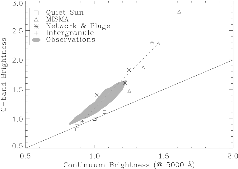
Figure 6: LTE syntheses of the G-band brightness produced by different model atmospheres at the disk center. The stars $*$ represent network and plage model atmospheres based on single fluxtubes (Chapman 1979; Solanki 1986; Bellot Rubio 1998). The triangles $\triangle$ correspond to model MISMAs (Sánchez Almeida & Lites 2000). Quiet Sun atmospheres are shown as squares $\Box$ (Gingerich et al. 1971; Vernazza et al. 1981; Maltby et al. 1986). The plus signs $+$ describe the intergranular environment of the G-band  bright points. The dotted line shows all possible locations of a magnetic concentration that is not spatially resolved. It has to be on the straight line that joins the fully resolved feature and the background; the actual position along this line is set by the filling factor. Observations by Berger et al. (1998b) are shown for reference (the shaded area). Atmospheres with equal contrast in the G-band  and continuum have to lie on the solid line. Everything has been normalized to the Maltby et al. quiet Sun.

Figure 6 shows synthetic G-band brightness versus (5000 Å) continuum intensity for model atmospheres of various kinds located at the solar disk center. It includes network and plage model atmospheres based on single fluxtubes (Chapman 1979; Solanki 1986; Bellot Rubio 1998), model MISMAs (Sánchez Almeida & Lites 2000), quiet Sun atmospheres (Gingerich et al. 1971; Vernazza et al. 1981; Maltby et al. 1986), and intergranules (modeled using stray light components of MISMAs; see Sánchez Almeida & Lites 2000). The latter are relevant since they represent the environment of the G-band  BPs. All intensities are normalized to the quiet Sun spectrum produced by the Maltby et al. (1986) atmosphere, that is very similar to the spectrum observed in the quiet Sun (see §3.3). Figure 6 also includes G-band observations with the best angular resolution available up to date (Figure 3 in Berger et al. 1998b). The white-light channel of these observations does not correspond to true continuum, though. The consequences of comparing white-light with continuum will be analyzed later.

First note that the G-band contrast in magnetic concentrations is about twice the continuum contrast. (For reference, the slope of the dotted line in Figure 6 amounts to 2.3.) This ratio of contrasts is in good agreement with observations (item # 1 in §4.1). There is, however, a serious discrepancy as far as the actual contrast is concerned. The synthetic spectra are much brighter than the observed BPs (item # 2 in §4.1). This discrepancy occurs in both white-light and G-band and can be understood if even the extremely high resolution data in which the observations are based do not yet resolve the BP. The hypothesis is reasonable since it stems from observations; point # 3 in §4.1. Assume this insufficient resolution. The observed brightness $I_{G}$ has contribution from both magnetic structures $I_{G}^{m}$ and intergranular background $I_{G}^{b}$. Then,

$$I_{G}=\xi I_{G}^{m}+(1-\xi)I_{G}^{b},$$ (20)

being $\xi$ the fraction of signal due to the magnetic concentrations. Similarly, the continuum intensity $I_{c}$ has also contribution from the BPs $I_{c}^{m}$ and the background $I_{c}^{b}$,

$$I_{c}=\xi I_{c}^{m}+(1-\xi)I_{c}^{b}.$$ (21)

According to equations (20) and (21), a spatially unresolved feature will show up in Figure 6 on the straight segment that joins the points corresponding to the fully resolved feature and the background. The exact position depends on $\xi$ which, in geometrical terms, corresponds to the fraction of this segment where the unresolved BP shows up. Figure 6 displays one of such straight lines, specifically, the one for a MISMA  and its intergranular background. It matches the range of observed contrasts for $\xi\leq 0.5$. The ability to account for the observed contrasts is shared by all model magnetic concentrations. All magnetic models in Figure 6 would cross the shaded area for reasonable values of the filling factor. This argument can be put forth in quantitative terms by combining equations (20) and (21) to form,

$$I_{G}-1=m~{}(I_{c}-1)+c,$$

$$m=(I_{G}^{m}-I_{G}^{b})/(I_{c}^{m}-I_{c}^{b}),$$ (22)

$$c=m~{}(1-I_{c}^{b})-(1-I_{G}^{b}).$$

As we pointed out above, MISMAs and single fluxtubes all yield,

$$m\approx 2.$$ (23)

A glance at the intergranular contrasts in Figure 6 indicates that $(1-I_{c}^{b})\sim(1-I_{G}^{b})\sim 0.1$, consequently, equations (22) and (23) render $c\sim 0.1$. The actual value is very uncertain but it has to be a small positive quantity, i.e.,

$$0<c\ll 1,$$ (24)

since $c=m~{}(1-I_{c}^{b})-(1-I_{G}^{b})\sim(m-1)(1-I_{G}^{b})\sim(1-I_{G}^{b})\ll 1$. The two results summarized in equations (23) and (24) compare well with the observed law (19), and this agreement does not depend on which model magnetic concentration is considered. (Obviously, we have assumed $I_{WL}=I_{c}$. The differences between the two quantities are analyzed below.)

Equations (22) and (24) can also explain the positive mean G-band contrast of magnetic regions having neutral continuum contrast (point # 6 in §4.1). Assuming $m$ and $c$ to be fairly constant across the magnetic region, then the relationship (22) applies to the mean quantities. Equations (22) and (24) predict $I_{G}=1+c>1$ when $I_{c}=1$.

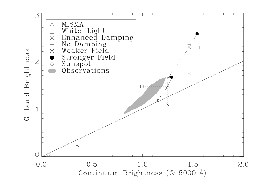
Figure 7: Displacements of the G-band brightness and continuum brightness caused by modifications of the model atmospheres. Two model MISMAs illustrate the common behavior. The original points are shown as triangles $\triangle$. The dotted lines join them with the various transformations. Including spectral lines in the continuum channel may increase or decrease the contrast; the continuum brightness of the brighter atmospheres become even larger and vice versa (squares $\Box$). Increasing the line wings reduces the G-band signals (times signs $\times$). Setting the damping to zero produces the plus signs $+$. Decreasing the magnetic field strength makes everything darker (stars $*$). The opposite happens when the field increases (black dots $\bullet$). Note that the brighter model atmosphere remains bright under all circumstances whereas the darker atmosphere sometimes does not. The diamonds correspond to sunspot umbrae. For the rest of the symbols, see Figure 6.

So far we have considered a few representative model magnetic concentrations. In addition to these syntheses, we carried out a set of simulations to find out how the synthetic contrasts in Figure 6 depend on details of the atmospheres. We used MISMA  model atmospheres with the claim that their behavior is representative of the other atmospheres. First, we explored how the position in the figure depends on using white-light instead of continuum intensity (except for the work by Koutchmy 1977, the white-light channel of the observations in §4.1 includes many spectral lines). We took a shortcut by replacing the true white-light band-pass with our G-band spectrum without CH lines (the G-band  synthesized considering only continuum and atomic lines). Two arguments justify the approximation. First, we just aim at a qualitative description. Second, the some 70 atomic lines included in our G-band modeling should be representative of a typical band-pass in the solar spectrum. Two results are shown in Figure 7. The original points, triangles, are to be compared with the new points, boxes. Including spectral lines in the band-pass induces two competing effects. The lines weaken with increasing temperature, which increases the white-light contrast with respect to the continuum contrast. On the contrary, the turbulence is enhanced in the magnetic atmospheres as compared with the quiet Sun (e.g., Solanki 1993; Sánchez Almeida & Lites 2000). This enhances the absorption of the saturated lines with respect to their absorption in the quiet Sun, decreasing the contrast in white-light. The first effect dominates in the brighter (hotter) atmospheres, where the lines are weak. The decrease of white-light contrast triumphs in the cooler atmospheres, though. Which tendency takes over depends on details of the atmosphere (in particular on the micro-turbulence).

Another source of error of the G-band synthesis is the damping wings of the lines, a very uncertain parameter. In the reference simulations of Figure 6 we borrowed the damping from the fit to the quiet Sun spectrum (§3.3). The damping in the quiet Sun is probably not the same as in magnetic concentrations and, since we are dealing with many saturated lines in the band-pass, moderate differences may play a significant role in determining the G-band absorption. To study the influence of the wings, we synthesized G-band spectra using a damping 0.5, instead of the 0.02 derived from the quiet Sun. The G-band brightness decreases as expected due to the global increase of absorption in the band-pass (see the times signs in Figure 7). This decrease dims so much the G-band signal of the cooler atmosphere in Figure 7 that it becomes even darker than the quiet Sun. Figure 7 includes the case with no damping for reference (the plus signs).

We have also varied the magnetic field strength of the original model MISMAs. Note that the influence of this parameter on the G-band brightness is not due to Zeeman effect, that we neglect (§3.2). The modifications result from the strong coupling of the thermodynamic parameters to the magnetic field strength. In particular, a reduction of field strength implies an increase of gas pressure to maintain the mechanical balance of the atmosphere (e.g., Sánchez Almeida & Lites 2000). An increase of gas pressure produces higher densities so the atmosphere is more opaque and the spectrum is formed higher up at lower temperatures. Consequently, the decrease of field strength lowers the contrasts. A 20% reduction is represented in Figure 7 using stars $*$. The augment of field strength leads to the opposite effect. We increase it up to 98 % of the maximum possible value, which induces the enhancement of contrast shown in Figure 7 with black dots $\bullet$. Such large field strength almost empties the magnetic components of the MISMAs, so that the spectra emerge from the non-magnetic components (see Sánchez Almeida 2000).

A simple conclusion follows from the exploratory simulations described above: the exact G-band synthetic contrast depends on details of the modeling difficult to constraint. If a model BP is bright enough then such details are secondary since the BP remains bright both in white-light and the G-band. However, such variations can modify the character of the concentrations that are not so bright. In particular, the relationship between continuum and G-band is expected to unsharpen or even break down for intrinsically low contrasts, where continuum BPs may or may not be G-band BPs depending on details of the atmosphere. In keeping with this conclusion, the fair correlation that we observe for weak contrasts is probably due to the limited angular resolution. It would be produced by intrinsically bright magnetic features mixed up with large amounts of dark background (as described by equation [22] with $I_{c}\gtrsim 1$). On the other hand, the expected fuzzy relationship between low contrast G-band BPs and contimuum BPs may be related to the diffuse G-band component (item # 5 in §4.1). The G-band signals would originate in concentrations whose properties lay on this ridge where to be or not to be bright depends on details.

Figure 7 includes the synthetic contrast produced by two model sunspot umbrae: the very cold model M in Maltby et al. (1986), and a hotter one (Collados et al. 1994). Unlike the quiet Sun magnetic concentrations studied up to now, the umbra G-band contrast is lower than the continuum contrast.

5 Corollaries of the LTE G-band modeling

5.1 Contribution functions for the G-band signals

The contribution functions ($CF$s) in equations (17) and (18) describe the atmospheric heights producing synthetic signals. Figure 8 shows continuum and G-band $CF$s in both a magnetic concentration and its intergranular environment. These $CF$s are normalized to render the signals in units of the quiet Sun signals. Moreover, the scale of heights is referred to the optical depth unity in the quiet Sun. The functions in Figure 8 illustrate the general behavior.

Note first that the G-band and the continuum $CF$s are similar so that they peak at the same heights (compare continuum and G-band $CF$s formed in the same atmospheres). Second, all $CF$s reach a maximum below the zero of the scale of heights. It is well below zero in the magnetic concentration because of the evacuation forced by the presence of a magnetic field (the so-called Wilson depression). On the other hand, the maxima of the intergranule $CF$s are very close to the quiet Sun $CF$s (that we do not represent in the figure). Problems of interpretation notwithstanding, the analogy between continuum and G-band $CF$s evidences that the corresponding signals come from neighboring atmospheric layers. This result agrees with observations. G-band and white-light images both show the solar granulation with identical appearance (see point # 7 in §4.1). Rutten (1999) points out that such similarity implies G-band signals being formed deep in the photosphere where the continuum is formed. We endorse his conclusion which should be regarded as an observational constraint. In our particular case, such observational requirements is fulfilled in a natural way.

The obvious difference between G-band and continuum $CF$s lies in their different widths, the G-band $CF$s being broader (Figure 8). This extended contribution follows from the varied range of opacities producing the G-band spectrum; from the cores of strong lines to the continuum.

5.2 Why are model magnetic concentrations so conspicuous in the G-band?

We found that the LTE spectrum in almost any model magnetic concentration explains the observed G-band enhancement (§4.2). This section sketches the radiative transfer effect that we believe to be responsible for such general behavior.

Figure 9 shows the variation with temperature of the absorption coefficients that are relevant for the LTE synthesis of the G-band and the continuum. It shows wavelength mean absorption coefficients at a constant density. The wavelength mean weights the absorption with the color filter in equation (15), whereas the density has been set to a value typical of the bottom of the quiet Sun photosphere. The actual filter and density do not modify the forthcoming qualitative arguments, though. A different filter barely changes the mean absorption. A different density shifts all the curves in the vertical direction (they approximately scale with the density within the range of temperatures represented in Figure 9). Note how the opacity in the G-band has a minimum at some 6000 K which, roughly speaking, represents the temperature of the layers that are observed in the quiet Sun. On the contrary, the continuum absorption coefficient does increase very rapidly with temperature. This different behavior explains why the model magnetic concentrations are much brighter in the G-band than in continuum. All the model magnetic concentrations are hotter than the quiet Sun in the layers producing the observed light. These larger temperatures enhance the continuum opacity, therefore, force the continuum photons to emerge from higher and therefore cooler layers. The net effect is a damping of the radiation field increase that would correspond to the sole augment of temperature. On the contrary, the opacity is barely modified in the G-band (it may even decrease). The temperature increase of the magnetic concentrations directly augments the radiation field that escapes from the atmosphere, enhancing the contrast of the magnetic concentrations when imaged in the G-band.

The neutral dependence of the G-band opacity on temperature is produced by the fortuitous opposite behavior of the continuum H^- opacity and the CH absorption. These two sources of opacity determine the net effect. The increase of H^- opacity with temperature is due to the increase of free electrons in the medium. The fall off of the CH opacity just follows the decrease of the CH abundance according to the Boltzmann factor in the dissociation equilibrium (equations [2] and [3]),

$$n_{\rm CH}\propto\exp[D_{0}/(kT)].$$ (25)

This dependence on the dissociation energy becomes clear upon inspection of Figure 9, where we include the approximate adsorption coefficient resulting from the sole action of $D_{0}$, namely,

$$\kappa_{CH}\simeq\kappa_{CH}(T_{0})\exp[D_{0}/(kT)-D_{0}/(kT_{0})],$$ (26)

with $T_{0}=6000$ K. It reproduces the behavior of the mean opacity in the region of interest. The discrepancy towards low temperatures (say below 5000 K) is due to the formation of CO molecules (see again Figure 9, the dotted line). The CO formation does not play a major role in our case, although it becomes critical in pores and sunspots (see §2.1).

To sum up, magnetic concentrations are so bright in the G-band because they are hot. The increase of temperature with respect to the quiet Sun is partly damped in the continuum, where the opacity also increases with temperature. The total G-band opacity barely depends on temperature, though.

6 Discussion and conclusions

Bright Points (BPs) in G-band images are associated with magnetic concentrations, although the physical cause of such brightness has been debated over the last years (see §1). The difficulties of understanding bear on the complications of modeling a molecular band, rather than on an enigmatic or unexpected behavior of the G-band signals. In order to explore the simplest possibility, we write and test a G-band LTE synthesis code that explicitly includes all the CH lines in the band-pass. As it was conjectured by Sánchez Almeida & Lites (2000), such simple LTE modeling seems to account for the main observational facts. Specifically, the G-band emerging from standard model magnetic concentrations is very bright relative to the quiet Sun. The G-band contrast is about twice the contrast of the same structures observed at continuum wavelength. The synthetic contrasts, however, exceed by far the observed contrasts. One can readily interpret this apparent contradiction if the observed G-band BPs are not yet spatially resolved. They have to fill 50% of the resolution elements or even less. Such requirement to match LTE syntheses and observations holds for all the semi-empirical model magnetic concentration that are available (from large fluxtubes to MISMAs; §4.2). The lack of enough resolution is not an ad-hoc assumption to fix up a conflict with observations; it actually comes out of the observations themselves (see §4.1). Insufficient resolution may also explain why the G-band contrast does not depend on the size of seemingly resolved G-band structures (§4.1). Each observed G-band BP would be a conglomerate of unresolved structures so that the actual observed contrast depends the degree of mixing with dark non-magnetic surroundings, rather than on the intrinsic contrast of the magnetic structures. Another possibility is the existence of a relationship between brightness and size masked because the inadequate resolution. Small bright features and large faint ones show up with the same apparent contrast (e.g., Title & Berger 1996).

Our purpose with this work is not just explaining the empirical relationship between magnetic concentrations and G-band BPs. Actually, we find it more interesting to find a reliable physical connection between the two phenomena that can be employed to build on. Once the physics of the association is well established, one can use modeling to examine the real diagnostic capabilities of the G-band BPs. Some of the calculations described in this paper begin to explore such possibility, and they already lead to several interesting results. We condense them here since they are scattered in main text. The G-band signals come from deep photospheric layers that barely differ from the layers that produce continuum photons (§5.1 and Figure 8). As it was advanced by Rutten (1999), the G-band opacity seems to be controlled by the dissociation of the CH molecule (see §5.2). The agent that determines this dissociation is not the radiation field, though. The densities in the photosphere are so high that the CH abundance is set by collisions with hydrogen (reactions [11] and [12]; see §2.3), photo-dissociation being secondary. Since the G-band results from absorption of saturated spectral lines, it very much depends on the line broadening parameters characterizing the atmosphere. Moderate changes of micro-turbulence and damping modify the G-band contrast. For large enough turbulence, magnetic concentrations may even show neutral contrast in the G-band (§4.2). It is therefore plausible that some of the real solar magnetic concentrations do not show up in G-band images. On the contrary, the continuum contrast does not depend on line broadenings and the magnetic concentrations will tend to be bright in continuum. We hypothesize the existence of low contrast continuum BPs without a G-band counterpart (§4.2). The LTE syntheses predict intrinsic G-band signals several times larger than those presently observed (§4.2). Consequently, we foresee an important augment of contrast upon improvement of the angular resolution of the observations. Finally, both single fluxtubes and MISMA model magnetic concentrations produce similar G-band brightness. This observable does not help discriminating between the different options of modeling unresolved magnetic concentrations.

We have shown that the synthetic LTE G-band spectra fulfil many observed properties of the G-band BPs. We have not shown that there is no other way to reproduce them. In particular, various alternatives mentioned in §1 still remain to be explored and therefore cannot be discarded.

While this paper was in preparation, we knew of two other groups carrying out LTE G-band syntheses in magnetic concentrations. They have advanced some results in recent meetings (e.g., Rutten et al. 2001; Steiner et al. 2001). As far as the overlapping with the present work is concerned, they find that specific model concentrations based on single fluxtubes present a G-band contrast larger than the continuum contrast. The values of these contrasts are similar to those computed in §4.2.

Figure 1: Abundance of the main diatomic molecules in the quiet Sun VAL-C model atmosphere. The variation with height of each species is normalized to its maximum value: 3.4 $\times\ 10^{13}$ cm^-3 for H₂, 2.4 $\times\ 10^{12}$ cm^-3 for CO, and 7.2 $\times\ 10^{9}$ cm^-3 for CH. Note that the CH peaks deep down in the atmosphere, just some 50 km above continuum optical depth unity at 5000 Å (which sets the zero of the abscissa; the small arrow on the top axis points out this height).

Figure 2: CH abundance deduced when considering different sets of molecules to solve the chemical equilibrium equations: H₂ and CH (the solid lines), H₂, CO and CH (the dotted lines) and up to 12 molecular species, including H₂, CO, CH (the dashed lines). The latter can be regarded as the exact solution. In the quiet Sun (a), even considering the sole formation of CH gives reasonable values. This approximation clearly breaks down in umbrae (b: Collados et al. 1994 model umbra). In this case, however, including just H₂ and CO renders good results.

Figure 3: Time evolution of the abundances of H₂, CH, CO, and OH (refer to the inset for the correspondence between type of line and species). This integration of the chemical evolution equations corresponds to typical photospheric conditions with no molecules at first (T= 6500 K and initial $n_{\rm H}=1.7\times 10^{17}$ cm^-3). The (thermodynamic) equilibrium CH abundance is reached within $10^{-5}$ s, a time-scale primarily set by the reactions that produce H₂ (see text and compare the solid and the dashed lines). Photo-dissociation seems to play a minor role in determining the CH abundance and so its exact rate does not modify these curves. All abundances, $n$, are referred to the abundance of atomic H, $n_{\rm H}$.

Figure 4: Quiet Sun spectrum including the G-band modeled here. The solid line corresponds to the observed solar spectrum at the disk center (Delbouille et al. 1973). The dashed line represents a best fit synthetic solar spectrum where the contribution of the atomic lines in the band pass has been neglected. Note the clear deficit of absorption at selected wavelengths. Compare this fit with Figure 5, where atomic lines are included. Wavelengths are given in Å, and the specific intensity is normalized to the continuum intensity at the solar disk center.

Figure 5: Portion of the quiet Sun solar spectrum comprising the G-band as we model it here. The solid line corresponds to the observed solar spectrum at the disk center (Delbouille et al. 1973). The dashed line shows the synthetic solar spectrum obtained with our LTE code (§3.3). It is normalized to the observed continuum intensity. The dotted line corresponds to the Gaussian color filter, 12 Å FWHM, that we use to model observations carried out in the G-band. Wavelengths are given in Å.

Figure 8: Contribution Functions of the G-band  and the 5000 Å continuum in a typical model MISMA. The $CF$s in the intergranular environment of the magnetic concentration are also included for comparison. Note that the G-band $CF$ in the MISMA  peaks at some -60 km, which is very close to the maximum of the continuum $CF$. The $CF$s have been normalized so that their areas yield the intensities referred to the quiet Sun (Maltby et al. model atmosphere). The inset on the upper right corner provides the equivalence between type of line and $CF$. The heights are referred to the continuum optical depth equals one in the quiet Sun.

Figure 9: Variation with temperature of the wavelength mean absorption coefficient. The dashed line represents the continuum absorption coefficient (mostly due to H^-). The solid line includes both the G-band absorption and the continuum, and it reaches a minimum at some 5900 K. The existence of this extreme explains the large contrast observed in the G-band (see text). The dotted line also represents the total absorption (G-band plus continuum), except that the formation of CO is turned off. As for the dash dot line, the G-band opacity is approximated by the Boltzmann factor of the dissociation equilibrium. The mass density $\rho$ has been set to a typical photospheric value (2 $\times\ 10^{-7}$ g cm^-3).

Table 1: Role of CH photo-dissociation in setting the chemical equilibrium.

T [K]	$\alpha_{photo}$ [s-1]	$\overline{t}$ [s]	$n_{H}$ [cm-3]	$r_{photo}$
4400	$1.65\times 10^{2}$	$6.1\times 10^{-3}$	$2.7\times 10^{15}$	$4.8\times 10^{-4}$
4400	$1.65\times 10^{2}$	$6.1\times 10^{-3}$	$1.2\times 10^{17}$	$1.1\times 10^{-5}$
6520	$4.05\times 10^{3}$	$2.5\times 10^{-4}$	$2.7\times 10^{15}$	$1.2\times 10^{-2}$
6520	$4.05\times 10^{3}$	$2.5\times 10^{-4}$	$1.2\times 10^{17}$	$2.6\times 10^{-4}$

References

- Allen (1973) Allen, C. W. 1973, Astrophysical Quantities (London: The Athlone Press)
- Bellot Rubio (1998) Bellot Rubio, L. R. 1998, Ph.D. thesis, Instituto de Astrofísica de Canarias, La Laguna
- Bennett (1988) Bennett, A. 1988, in Rate Coefficients in Astrochemistry, ed. T. J. Millar & D. A. Williams (Dordrecht: Kluwer), 339
- Berger et al. (1998a) Berger, T. E., Löfdahl, M. G., Shine, R. A., & Title, A. M. 1998a, ApJ, 506, 439
- Berger et al. (1998b) Berger, T. E., Löfdahl, M. G., Shine, R. A., & Title, A. M. 1998b, ApJ, 495, 973
- Berger et al. (1995) Berger, T. E., Schrijver, C. J., Shine, R. A., Tarbell, T. D., Title, A. M., & Scharmer, G. 1995, ApJ, 454, 531
- Berger & Title (1996) Berger, T. E., & Title, A. M. 1996, ApJ, 463, 365
- Bonet (1999) Bonet, J. A. 1999, in ASSL, Vol. 239, Motions in the Solar Atmosphere, ed. A. Hanslmeier & M. Messerotti (Dordrecht: Kluwer), 1
- Chapman (1979) Chapman, G. A. 1979, ApJ, 232, 923
- Collados et al. (1994) Collados, M., Martínez Pillet, V., Ruiz Cobo, B., del Toro Iniesta, J. C., & Vázquez, M. 1994, A&A, 291, 622
- Cox & Giuli (1968) Cox, J. P., & Giuli, R. T. 1968, Principles of Stellar Structure (New York: Gordon & Breach)
- de Boer & Kneer (1992) de Boer, C. R., & Kneer, F. 1992, A&A, 264, L24
- Delbouille et al. (1973) Delbouille, L., Roland, G., & Neven, L. 1973, Photometric Atlas of the Solar Spectrum (Liège: Institut d’Astrophysique de L’Université de Liège)
- Draine (1978) Draine, B. T. 1978, ApJS, 36, 595
- Dunn & Zirker (1973) Dunn, R. B., & Zirker, J. B. 1973, Sol. Phys., 33, 281
- Edlén (1966) Edlén, B. 1966, Metrologia, 2, 71
- Gear (1971) Gear, C. N. 1971, Numerical Initial Value Problems in Ordinary Differential Equations (Englewoods Cliffs, NJ: Pertice-Hall)
- Gingerich et al. (1971) Gingerich, O., Noyes, R. W., Kalkofen, W., & Cuny, Y. 1971, Sol. Phys., 18, 347
- Grevesse (1984) Grevesse, N. 1984, Phys. Scr, T8, 49
- Hearnshaw (1973) Hearnshaw, J. B. 1973, A&A, 28, 279
- Illing (1981) Illing, R. M. E. 1981, ApJ, 248, 358
- Jørgensen et al. (1996) Jørgensen, U. G., Larsson, M., Iwamae, A., & Yu, B. 1996, A&A, 315, 204
- Keenan (1942) Keenan, P. C. 1942, ApJ, 96, 101
- Konnov (2000) Konnov, A. A. 2000, Detailed reaction mechanism for small hydrocarbons combustion. release 0.5, http://homepages.vub.ac.be/$∼$akonnov/
- Koutchmy (1977) Koutchmy, S. 1977, A&A, 61, 397
- Kunasz & Auer (1988) Kunasz, P., & Auer, L. H. 1988, J. Quant. Spec. Radiat. Transf., 39, 67
- Kurucz et al. (1987) Kurucz, R. L., van Dishoeck, E. F., & Tarafdar, S. P. 1987, ApJ, 322, 992
- Löfdahl et al. (1998) Löfdahl, M. G., Berger, T. E., Shine, R. S., & Title, A. M. 1998, ApJ, 495, 965
- Magain (1986) Magain, P. 1986, A&A, 163, 135
- Maltby et al. (1986) Maltby, P., Avrett, E. H., Carlsson, M., Kjeldseth-Moe, O., Kurucz, R. L., & Loeser, R. 1986, ApJ, 306, 284
- Mehltretter (1974) Mehltretter, J. P. 1974, Sol. Phys., 38, 43
- Muller & Roudier (1984) Muller, R., & Roudier, T. 1984, Sol. Phys., 94, 33
- Press et al. (1988) Press, W. H., Flannery, B. P., Teukolsky, S. A., & Vetterling, W. T. 1988, Numerical Recipes (Cambridge: Cambridge University Press)
- Roberge et al. (1981) Roberge, W. G., Dalgarno, A., & Flannery, B. P. 1981, ApJ, 243, 817
- Russell (1934) Russell, H. N. 1934, ApJ, 79, 317
- Rutten (1999) Rutten, R. J. 1999, in Third Advances in Solar Physics Euroconference: Magnetic Fields and Oscillations, ed. B. Schmieder, A. Hofmann, & J. Staude, ASP Conf. Ser. 184 (San Francisco: ASP), 181
- Rutten et al. (2001) Rutten, R. J., Kiselman, D., & Plez, B. 2001, in Advanced Solar Polarimetry: Theory, Instrumentation and Modeling, ed. M. Sigwarth, ASP Conf. Ser. (San Francisco: ASP), in press
- Sánchez Almeida (1992) Sánchez Almeida, J. 1992, Sol. Phys., 137, 1
- Sánchez Almeida (1997) Sánchez Almeida, J. 1997, ApJ, 491, 993
- Sánchez Almeida (1998) Sánchez Almeida, J. 1998, in Three-Dimensional Structure of Solar Active Regions, ed. C. E. Alissandrakis & B. Schmieder, ASP Conf. Ser. 155 (San Francisco: ASP), 54
- Sánchez Almeida (2000) Sánchez Almeida, J. 2000, ApJ, 544, 1135
- Sánchez Almeida et al. (1996) Sánchez Almeida, J., Landi Degl’Innocenti, E., Martínez Pillet, V., & Lites, B. W. 1996, ApJ, 466, 537
- Sánchez Almeida & Lites (2000) Sánchez Almeida, J., & Lites, B. W. 2000, ApJ, 532, 1215
- Sánchez Almeida et al. (1996) Sánchez Almeida, J., Ruiz Cobo, B., & del Toro Iniesta, J. C. 1996, A&A, 314, 295
- Sánchez Almeida & Trujillo Bueno (1999) Sánchez Almeida, J., & Trujillo Bueno, J. 1999, ApJ, 526, 1013
- Sauval & Tatum (1984) Sauval, A. J., & Tatum, J. B. 1984, ApJS, 56, 193
- Schmidt-Kaler (1982) Schmidt-Kaler, T. 1982, in Landolt-Börnstein, Vol. 2b, Astronomy and Astrophysics, ed. K. Schaifers & H. H. Voigt (Berlin: Springer-Verlag), 1
- Solanki (1986) Solanki, S. K. 1986, A&A, 168, 311
- Solanki (1993) Solanki, S. K. 1993, Space Science Rev., 63, 1
- Steiner et al. (2001) Steiner, O., Bruls, J., & Hauschildt, P. H. 2001, in Advanced Solar Polarimetry: Theory, Observations and Instrumentation, ed. M. Sigwarth, ASP Conf. Ser. (San Francisco: ASP), in press
- Stenflo (1982) Stenflo, J. O. 1982, Sol. Phys., 80, 209
- Stenflo & Lindegren (1977) Stenflo, J. O., & Lindegren, L. 1977, A&A, 59, 367
- Tejero Ordóñez & Cernicharo (1991) Tejero Ordóñez, J., & Cernicharo, J. 1991, Modelos de Equilibrio Termodinámico Aplicados a Envolturas Circunestelares de Estrellas Evolucionadas (Madrid: Instituto Geográfico Nacional)
- Title & Berger (1996) Title, A. M., & Berger, T. E. 1996, ApJ, 463, 797
- Tsuji (1964) Tsuji, T. 1964, Ann. Tokyo. Astron. Obs., 2nd ser. 9, 1
- Tsuji (1973) Tsuji, T. 1973, A&A, 23, 411
- van Ballegooijen et al. (1998) van Ballegooijen, A. A., Nisenson, P., Noyes, R. W., Löfdahl, M. G., Stein, R. F., Nordlund, Å., & Krishnakumar, V. 1998, ApJ, 509, 435
- van Dishoeck (1987a) van Dishoeck, E. F. 1987a, J. Chem. Phys., 86, 196
- van Dishoeck (1987b) van Dishoeck, E. F. 1987b, in Astrochemistry, ed. M. S. Vardya & S. P. Tarafdar, IAU Symp. 120 (Dordrecht: Reidel), 51
- van Dishoeck & Blake (1998) van Dishoeck, E. T., & Blake, G. A. 1998, ARA&A, 36, 317
- Vela Villahoz et al. (1994) Vela Villahoz, E., Sánchez Almeida, J., & Wittmann, A. D. 1994, A&AS, 103, 293
- Vernazza et al. (1981) Vernazza, J. E., Avrett, E. H., & Loeser, R. 1981, ApJS, 45, 635
- Yi et al. (1993) Yi, Z., Jensen, E., & Engvold, O. 1993, in ASP Conf. Ser., Vol. 46, The Magnetic and Velocity Fields of Solar Active Regions, ed. H. Zirin, G. Ai, & H. Wang, San Francisco, 232