Distances in inhomogeneous quintessence cosmology

We investigate the properties of cosmological distances in locally inhomogeneous universes with pressureless matter and dark energy (quintessence), with constant equation of state, $p_{X}=w_{X}\rho_{X}$, $-1\leq w_{X}<0$. We give exact solutions for angular diameter distances in the empty beam approximation. In this hypothesis, the distance-redshift equation is derived fron the multiple lens-plane theory. The case of a flat universe is considered with particular attention. We show how this general scheme makes distances degenerate with respect to $w_{X}$ and the smoothness parameters $\alpha_{i}$, accounting for the homogeneously distributed fraction of energy of the $i-$components. We analyse how this degeneracy influences the critical redshift where the angular diameter distance takes its maximum, and put in evidence future prospects for measuring the smoothness parameter of the pressureless matter, $\alpha_{M}$.

e-mail addresses:
sereno@na.astro.it
covone@na.infn.it
ester@na.infn.it

1 Introduction

Recent measurements of the cosmic microwave background anisotropy [de Bernardis et al. 2000] strongly support the flat universe predicted by inflationary cosmology. At the same time, there are strong evidences, i.e. from dynamical estimates or X-ray and lensing observations of clusters of galaxies, that the today pressureless matter parameter of the universe $\Omega_{M}$ is significantly less than unity ($\Omega_{M}=\Omega_{CDM}+\Omega_{B}\simeq[0.30{\pm}0.10]+[0.04{\pm}0.01]$, where CDM and B respectively stand for cold dark matter and baryons), while the hot matter (photons and neutrinos) is really neglectable. Flatness so requires another positive contribute to the energy density of the universe, the so called dark energy – see, for example, Silveira & Waga [Silveira & Waga 1997] or Turner & White [Turner & White 1997] – that, according to the recent data from SNIa [Riess et al. 1998, Perlmutter et al. 1999], must have negative pressure to account for an accelerated expanding universe. One of the possible solutions of this puzzle is the $\Lambda$CDM universe where the fraction $\Omega_{X}$ of the dark energy is supported by a cosmological constant $\Lambda$. A very promising altervative, the quintessence, was proposed by Caldwell, Dave & Steinhardt [Caldwell et al. 1998] in the form of a dynamical, spatially inhomogeneous energy with negative pressure, i.e. the energy of a slowly evolving scalar field with positive potential energy. Apart from flatness, a scalar field coupled to matter through gravitation can also explain the so called coincidence problem, that is, it can provide a mechanism to make the today densities of matter and dark energy comparable. As shown in Wang et al. [Wang at al. 2000], a large set of indipendent observations agrees with a universe described in terms of pressureless matter and quintessence only, a hypothesis that we will make in this paper.

A scalar field is not an ideal adiabatic fluid [Grishchuk 1994, Caldwell et al. 1998] and the sound speed in it varies with the wavelength in such a way that high frequency modes remain stable still when $w_{X}<0$. Moreover, smoothness is gauge dependent, and so a fluctuating inhomogeneous energy component is naturally defined [Caldwell et al. 1998]. Inhomogeneities, both in quintessence and CDM, make the relations for the distances derived in Friedmann-Lemaître-Robertson-Walker (FLRW) models not immediately applicable to the interpetration of experimental data both in measurements of luminosity distances and angular diameter distances. The observed universe appears to be homogeneously distributed only on large scales ($\stackrel{{\scriptstyle>}}{{\sim}}500$ Mpc), while the propagation of light is a local phenomena. In lack of a really satisfactory exact solution for inhomogeneous universes in the framework of General Relativity [Krasiński 1997], the usual, very simple framework we shall adopt for the study of distances is the on average FLRW universe (Schneider, Ehlers & Falco 1992; Seitz, Schneider & Ehlers 1994), where: i) the relations on a large scale are the same of the corresponding FLRW universe; ii) the anisotropic distortion of the bundle of light rays contributed by external inhomogeneities (the shear $\sigma$) is not significant; iii) only the fraction $\alpha_{i}$, the so called smoothness parameter, of the $i$-component contributes to the Ricci focusing ${\cal R}$, that is to the isotropic focusing of the bundle. The distance recovered in this ’empty beam approximation’, sometimes known as Dyer-Roeder (DR) distance, has been long studied (Zel’dovich 1964; Kantowski 1969; Dyer & Roeder 1972, 1973; Linder 1988) and now is becoming established as a very useful tool for the interpretation of experimental data (Kantowski 1998; Kantowski & Thomas 2000; Perlmutter et al. 1999; Giovi, Occhionero & Amendola 2000). For a very large sample of standard candles, as SNIa for luminosity distance, or standard rods, as compact radio sources for angular diameter distances (Gurvits, Kellermann & Frey 1999), the effects of overdensity and underdensity along different lines of sight between observer and sources balance each other out, and the mean distance of the probability distribution of distances for fixed source redshift, corresponding to the FLRW distance, can be used (Wang 1999, 2000). Nevertheless, for the present quite poor samples, sources are very rarely brightened by the gravitational effect of occurring overdense clumps, and so, for propagation of light far from local inhomogeneities, the source appears dimmer and smaller with respect to the homogeneous case. So the distance to be used is the mode of the distribution, that is, in a very good approximation, the DR distance [Schneider et al. 1992, Kantowski 1998]. In general, the smoothness parameters for matter and quintessence (respectively $\alpha_{M}$ and $\alpha_{X}$) and the equation of state $w_{X}$ are redshift dependent, but they can be considered, in the redshift interval covered by observations, as constant. For the clumpiness parameters, the constancy is motivated by the absence of significant variations in the development of structures in the observed redshift range. Instead, also in presence of redshift variations in $w_{X}$, only its integral properties have effect on the distance. In fact, in flat FLRW models the distance depends on $w_{X}$ only through a triple integral on the redshift (Maor, Brustein & Steinhardt 2000). Hereafter, we will consider the $\alpha_{i}$ and $w_{X}$ as constant. For the cosmological constant $w_{X}=-1$; a network of light, nonintercommuting topological defects [Vilenkin 1984, Spergel & Pen 1997] gives $w_{X}=-m/3$ where $m$ is the dimension of the defect: for a string $w_{X}=-1/3$, for a domain wall $w_{X}=-2/3$; an accelerated universe requires $w_{X}<-1/3$.

In this approximation, distances are functions of a family of parameters: $\Omega_{M}$ and $\Omega_{X}$, which describe the energy content of the universe on large scales; $w_{X}$, which describes the equation of state of the quintessence and varies between $-1$ and $0$; two clumpiness parameters, $\alpha_{M}$ and $\alpha_{X}$, representing the degree of homogeneity of the universe and which are to be used for phenomena of local propagation.

This paper is organized as follows: in Sect.2 we introduce the so called DR equation and discuss some features and its solution for quintessence in the form of topological defects; Sect.3 lists the general solution for the DR equation in the flat case and some simple expressions in extreme situations; in Sect.4 the multiple lens-plane theory of gravitational lensing is applied for a derivation of the DR equation without using the focusing equation; Sect.5 is devoted to the degeneracy of the distance with respect to the various parameters; in Sect.6 the critical redshift at which the angular diameter distance takes its maximum is studied, and, at last, in Sect.7 we draw the conclusions.

2 The beam equation for inhomogeneous quintessence

In the hypotheses discussed above, the focusing equation [Sachs 1961, Schneider et al. 1992] for the angular diameter distance $D_{A}$ in terms of an affine parameter $\lambda$,

$$\frac{d^{2}D_{A}}{d\lambda^{2}}=-(|\sigma(\lambda)|^{2}-{\cal R}(\lambda))D_{A},$$ (1)

becomes (see also Linder 1988)

$$\frac{d^{2}D_{A}}{d\lambda^{2}}+\frac{1}{2}(1+z)^{2}\left[3\alpha_{M}\Omega_{M}(1+z)^{3}+n_{X}\alpha_{X}\Omega_{X}(1+z)^{n_{X}}\right]D_{A}=0,$$ (2)

where $n_{X}\equiv 3(w_{X}+1)$ ($0<n_{x}<3$), and the relation between $\lambda$ and the redshift $z$, in terms of the generalized Hubble parameter

$$H(z)=H_{0}\sqrt{\Omega_{M}(1+z)^{3}+\Omega_{X}(1+z)^{n_{X}}+\Omega_{K}(1+z)^{2}},\ \Omega_{K}\equiv 1-\Omega_{M}-\Omega_{X},$$ (3)

is

$$\frac{dz}{d\lambda}=(1+z)^{2}\frac{H(z)}{H_{0}}.$$ (4)

The isotropic focusing effect in equation (2) is simply represented by the multiplicative factor to $D_{A}$; this coefficient increases with $\alpha_{M}$, $\alpha_{X}$ and $n_{X}$.

Equation (2) is sometimes called the generalized DR equation. Substituting for $\lambda$ in equation (2) by using equation (4), we have

$$H^{2}(z)\frac{d^{2}D_{A}}{dz^{2}}+\left[\frac{2H^{2}(z)}{1+z}+\frac{1}{2}\frac{dH^{2}}{dz}\right]\frac{D_{A}}{dz}+\frac{1}{2}(1+z)\left[3\alpha_{M}\Omega_{M}+n_{X}\alpha_{X}\Omega_{X}(1+z)^{n_{X}-3}\right]D_{A}=0;$$ (5)

the initial conditions on equation (5) are

$$D_{A}(z_{d},z_{d})=0,$$ (6)

$$\left.\frac{d}{dz}D_{A}(z_{d},z)\right|_{z=z_{d}}=\frac{1}{1+z_{d}}\frac{c}{H(z_{d})},$$

where $D_{A}(z_{d},z)$ is the angular diameter distance between $z_{d}$ (that, in general, can be different from zero, as occurs in gravitational lensing for the deflector) and the source at $z$.

Changing to the expansion factor $a\equiv 1/(1+z)$, equation (5) is

$$a^{2}\left[\Omega_{M}+\Omega_{X}a^{3-n_{X}}+\Omega_{K}a\right]\frac{d^{2}D_{A}}{da^{2}}-a\left[\frac{3}{2}\Omega_{M}+\frac{n_{X}}{2}\Omega_{X}a^{3-n_{X}}+\Omega_{K}a\right]\frac{dD_{A}}{da}$$

$$+\left[\alpha_{M}\frac{3}{2}\Omega_{M}+\alpha_{X}\frac{n_{X}}{2}\Omega_{X}a^{3-n_{X}}\right]D_{A}=0,$$ (7)

a form which will be useful in the next sections.

In a generic space-time, the angular diameter distance $D_{A}$ and the luminosity distance $D_{L}$ are related by (Etherington 1933)

$$D_{L}=(1+z)^{2}D_{A},$$ (8)

so that the considerations we will make about $D_{A}$ are easily extended to $D_{L}$.

2.1 Exact solutions for $\Omega_{K}\neq 0$

The observational data nowadays available are in agreement with the hypothesis of a flat universe, but are also compatible with a non zero, although small, value of $\Omega_{K}$. A small value of $\Omega_{K}$ is also allowed by the inflationary theory. These circumstances make useful the study of the effect of the curvature on the cosmological distances since today technology allows to put strong constraints on the cosmological parameters.

For $\alpha_{X}=1$, equation (2) reduces to

$$a^{2}(\Omega_{M}+\Omega_{K}a+\Omega_{X}a^{3-n_{X}})\frac{d^{2}D_{A}}{da^{2}}-a\left(\frac{3}{2}\Omega_{M}+\Omega_{K}a+\frac{n_{X}}{2}\Omega_{X}a^{3-n_{X}}\right)\frac{dD_{A}}{da}+$$

$$\left(\frac{3}{2}\alpha_{M}+\frac{n_{X}}{2}\Omega_{X}a^{3-n_{X}}\right)D_{A}=0.$$ (9)

To solve equation (2.1), we proceed as in Demiasnki et al. [Demianski et al. 2000]. First, we look for a solution in the power form $a^{s}$ when $\Omega_{X}=\Omega_{K}=0$. The parameter $s$ is constrained to fulfill the algebraic equation

$$s^{2}-\frac{5}{2}s+\frac{3}{2}\alpha_{M}=0,$$ (10)

which has the solutions

$$s_{\pm}=\frac{5}{4}{\pm}\frac{1}{4}\sqrt{25-24\alpha_{M}}\equiv\frac{5}{4}{\pm}\beta.$$ (11)

When $\Omega_{X}\not=0$, $\Omega_{K}\not=0$, we choose to impose the form $D_{A}=a^{s}f(a)$ to the solution, being $f$ a generic function. Inserting this expression into equation (2.1) we have for $f$

$$a\left(\Omega_{M}+\Omega_{K}a+\Omega_{X}a^{3-n}\right)\frac{d^{2}f}{da^{2}}-\frac{df}{da}\left(\Omega_{M}(2s-\frac{3}{2})+\Omega_{K}(2s-1)a\right.$$ (12)

$$+\left.\left(s(s-1)-\frac{n_{X}}{2}s\right)\Omega_{X}a^{3-n_{X}}\right)+(\Omega_{K}s(s-2)+\Omega_{X}(s^{2}-s(1+\frac{n_{X}}{2}))a^{2-n_{X}})f=0.$$

The initial conditions at $a=1$ for the auxiliary function $f$ come out from equation (6) evaluated at $z=0$,

$$f(1)=0,$$ (13)

$$\left.\frac{d}{dz}f(a)\right|_{a=1}=\frac{c}{H_{0}}.$$

Equation (2.1) is very useful to obtain some exact solutions of the DR equation, corresponding to integer values of the quintessence parameter $n_{X}$. Since the solutions for the case of the cosmological constant, $n_{X}=0$ [Kantowski 1998], and for the pressureless matter, $n_{X}=3$ [Seitz & Schneider 1994], are already known, we will consider only string networks, $n_{X}=2$ $(w_{X}=-1/3)$ and the domain walls with $n_{X}=1$ $(w_{X}=-2/3)$. Let us start with the case $n_{X}=2$, when equation (2.1) reduces to

$$a(c_{1}+c_{2}a)\frac{d^{2}f}{da^{2}}+(c_{3}+c_{2}c_{4}a)\frac{df}{da}+c_{5}f==0,$$ (14)

being

$$c_{1} = \Omega_{M},$$

$$c_{2} = \Omega_{K}+\Omega_{X},$$

$$c_{3} = c_{2}\left(2s-\frac{3}{2}\right),$$

$$c_{4} = 2s-1,$$

$$c_{5} = \Omega_{K}s(s-2)+\Omega_{X}\left(s\left(s-\frac{3}{2}+\frac{1}{2}\right)\right).$$ (15)

Equation  (14) is of hypergeometric type, i.e. it has three regular singularities [Ince 1956], and so, for $n_{X}=2$, $f$ is the hypergeometric function. If we indicate with $f_{s_{+}}$ and $f_{s_{-}}$ two indipendent solutions for, respectively, $s=s_{+}$ and $s=s_{-}$, we can write the general solution of equation (2.1) for $n_{X}=2$ as

$$D_{A} = A_{+}a^{s_{+}}f_{s_{+}}(a)+A_{-}a^{s_{-}}f_{s_{-}}\left(a\right)$$ (16)

$$= \frac{1}{(1+z)^{5/4}}\left(A_{+}(1+z)^{-\beta}f_{s_{+}}\left(\frac{1}{1+z}\right)+A_{-}\left(1+z\right)^{\beta}f_{s_{-}}\left(\frac{1}{1+z}\right)\right),$$

where $A_{+}$ and $A_{-}$ are constants determined by the initial conditions. In equation (16) we have expressed the scale factor, $a$, in terms of the redshift.

Let us consider now the case $n_{X}=1$, when the equation for $f$ becomes

$$a\left(\frac{\Omega_{M}}{\Omega_{X}}+\frac{\Omega_{K}}{\Omega_{X}}a+a^{2}\right)\frac{d^{2}f}{da^{2}}$$ (19)

$$+\left(\frac{\Omega_{M}}{\Omega_{X}}\left(2s-\frac{3}{2}\right)+\frac{\Omega_{K}}{\Omega_{X}}\left(2s-1\right)a+\left(2s-\frac{1}{2}\right)a^{2}\right)\frac{df}{da}$$

$$+\left(\frac{\Omega_{K}}{\Omega_{X}}s\left(s-2\right)+\left(s\left(s-2\right)+\frac{1}{2}\right)a\right)f=0.$$

Equation (19) is a fuchsian equation with three finite regular points plus a regular singularity at $\infty$ [Ince 1956]. The regular points in the finite part of the complex plane are

$$a_{1} = 0,$$

$$a_{2} = \frac{-\Omega_{K}-\sqrt{\Omega_{K}^{2}-\Omega_{M}\Omega_{X}}}{2},$$ (20)

$$a_{3} = \frac{-\Omega_{K}+\sqrt{\Omega_{K}^{2}-\Omega_{M}\Omega_{X}}}{2}.$$

The trasformation $y=a/a_{2}$ sends $a_{2}\rightarrow 1$ and $a_{2}\rightarrow\zeta=\frac{a_{3}}{a_{2}}$. In terms of $y$, equation  (19) is

$$y\left(y-1\right)\left(y-\zeta\right)\frac{{d^{2}f}{dy^{2}}}{+}\left(\frac{\Omega_{M}}{\Omega_{X}}(2s-\frac{3}{2})+\frac{\Omega_{K}}{\Omega_{X}}(2s-1)a_{2}y\right)$$

$$\quad+\left((2s-\frac{1}{2}){a_{2}}^{2}{y}^{2}\right)\frac{df}{dy}+\left(\frac{\Omega_{K}}{a_{2}\Omega_{X}}s(s-2)+\left(s(s-2)+\frac{1}{2}\right)a_{2}y\right)f=0,$$ (21)

which can be reduced to the standard form

$$\frac{d^{2}f}{dy^{2}}+\left(\frac{\gamma}{y}+\frac{\delta}{y-1}+\frac{\epsilon}{y-\zeta}\right)\frac{df}{dy}+\left(\frac{\theta\lambda y-q}{y\left(y-1\right)\left(y-\zeta\right)}\right)f=0,$$ (22)

where

$$\gamma+\delta = \left(2s-\frac{1}{2}\right)a_{2}^{2},$$

$$\frac{\Omega_{K}}{\Omega_{X}}\left(2s-1\right)a_{2} = \gamma\left(1+\zeta\right)+\delta\zeta+\epsilon,$$

$$\gamma\zeta = \frac{\Omega_{M}}{\Omega_{X}}\left(2s-\frac{3}{2}\right),$$ (23)

$$q = \frac{\Omega_{K}}{\Omega_{M}}s\left(s-2\right),$$

$$\theta\lambda = s\left(s-\frac{3}{2}\right)+\frac{1}{2}.$$

Equation (22) is the Heun equation [Erdélyi et al. 1955], which is slightly more complicated then the hypergeometric equation, possessing four points of regular singularity in the entire complex plain, rather than three. The constant $q$ is the so called accessory parameter, whose presence is due to the fact that a fuchsian equation is not completely determined by the position of the singularities and the indices. The Heun equation can be charaterized by a ${\cal P}$ symbol, and the solutions can be expanded in series of hypergeometric functions. Thus, the solution of the equation  (2.1) for $n_{X}=1$ can be formally written as equation  (16), once the functions $f_{s_{+}}$ and $f_{s_{-}}$ are interpreted as Heun functions.

In Fig. LABEL:fig1, we plot the solutions found above.

3 Exact solutions for $\Omega_{K}=0$

The DR equation for a flat universe has already been solved considering the limiting case of the cosmological constant [Kantowski 1998, Kantowski & Thomas 2000, Demianski et al. 2000]. Here, in presence of generic quintessence, we propose the general solution in terms of hypergeometric functions and, then, list particular solutions in terms of elementary functions.

3.1 General solution

When $\Omega_{K}=0$, equation (2) reduces to

$$\left(a^{2}(\Omega_{M}+(1-\Omega_{M})a^{3-n_{X}})\right)\frac{d^{2}D_{A}}{da^{2}}-a\left(\frac{3}{2}\Omega_{M}+\frac{n_{X}}{2}(1-\Omega_{M})a^{3-n_{X}}\right)\frac{dD_{A}}{da}$$

$$+\left(\frac{3}{2}\alpha_{M}\Omega_{M}+\frac{n_{X}}{2}\alpha_{X}(1-\Omega_{M})a^{3-n_{X}}\right)D_{A}=0;$$ (24)

dividing equation (3.1) by $\Omega_{M}$ and defining $\mu\equiv\frac{1-\Omega_{M}}{\Omega_{M}}$, we have

$$a^{2}(1+\mu a^{3-n_{X}})\frac{d^{2}D_{A}}{da^{2}}-a\left(\frac{3}{2}+\frac{n_{X}}{2}\mu a^{3-n_{X}}\right)\frac{dD_{A}}{da}+\left(\frac{3}{2}\alpha_{M}+\frac{n_{X}}{2}\alpha_{X}\mu a^{3-n_{X}}\right)D_{A}=0.$$ (25)

To solve equation (25), we proceed as in Sect.2.1. First, we look for a solution in the power form $a^{s}$ when $\mu=0$. The parameter $s$ is constrained to fulfill equation (10). When $\mu\not=0$, we choose to impose the form $D_{A}=a^{s}f(a)$ to the solution, where $f$ is generic. Inserting this expression into equation (25) and changing to $x\equiv a^{3-n_{X}}$, we have for $f$

$$x(3-n_{X})(1+\mu x)\frac{d^{2}f}{dx^{2}}+\left(\left(2s-n_{X}+\frac{1}{2}\right)+\left(2-\frac{3}{2}n_{X}+2s\right)\mu x\right)\frac{df}{dx}$$

$$+\frac{\mu}{2}\left(s-\frac{3\alpha_{M}-n_{X}\alpha_{X}}{3-n_{X}}\right)f=0.$$ (26)

Again, this equation can be solved in terms of hypergeometric functions. Denoting with $f_{s_{+}}$ and $f_{s_{-}}$ two of such indipendent solutions for, respectively, $s=s_{+}$ and $s=s_{-}$, we can write the general solution of equation (3.1) as

$$D_{A}=A_{+}a^{s_{+}}f_{s_{+}}(x(a))+A_{-}a^{s_{-}}f_{s_{-}}(x(a))$$

(27)

$$=\frac{1}{(1+z)^{5/4}}\left(A_{+}(1+z)^{-\beta}f_{s_{+}}\left(\frac{1}{(1+z)^{3-n_{X}}}\right)+A_{-}(1+z)^{\beta}f_{s_{-}}\left(\frac{1}{(1+z)^{3-n_{X}}}\right)\right),$$

where $A_{+}$ and $A_{-}$ are constants determined by the initial conditions.

3.2 Particular cases

Once we have the general solution of equation (3.1) in terms of hypergeometric functions, we go now to list some expressions of the angular diameter distance in terms of elementary functions in two extremal cases.

3.2.1 Homogeneous universe

In this case we have that $\alpha_{M}=\alpha_{X}=1$, so that the angular diameter distance takes the form valid in a FLRW universe, that is

$$D_{A}(z_{d},z)=\frac{c}{H_{0}}\frac{1}{1+z}\int_{z_{d}}^{z}\frac{dz^{{}^{\prime}}}{\sqrt{\Omega_{M}(1+z^{{}^{\prime}})^{3}+(1-\Omega_{M})(1+z^{{}^{\prime}})^{n_{X}}}}.$$ (28)

This is the integral of the differential binomial

$$x^{\mu}(a+bx^{\nu})^{\rho},$$ (29)

where $x=1+z,\ a=\Omega_{M},\ b=1-\Omega_{M},\ \mu=-3/2,\ \nu=n_{X}-3$ and $\rho=-1/2$. We can put this integral in rational form when

$$n_{X}=\frac{3s-1}{s},\ s\in{\cal Z}-\{0\},$$ (30)

performing the substitutions (Picone & Miranda 1943)

$$t=\sqrt{\Omega_{M}+(1+\Omega_{M})(1+z)^{n_{X}-3}}$$

when $s$ is even and

$$t=\sqrt{\frac{\Omega_{M}+(1+\Omega_{M})(1+z)^{n_{X}-3}}{(1+z)^{n_{X}-3}}}$$

for odd $s$. Equation (30) includes all and only the rational values of $n_{X}$ for which equation (28) can be solved in terms of elementary functions. $n_{X}$ varies from $2$ ($w_{X}=-1/3$), when quintessence evolves like curvature, to $4$ ($w_{X}=1/3$)(hot dark matter); for $s\rightarrow{\pm}\infty$, $n_{X}$ tends to $3$, giving ordinary pressureless matter. For $n_{X}=2$ (see also Lima & Alcaniz 2000) we get

$$D_{A}(z_{d},z)=\frac{c}{H_{0}}\frac{2}{(1+z)\sqrt{1-\Omega_{M}}}\left[{\rm Arctanh}\left(\frac{\sqrt{1+\Omega_{M}z}}{\sqrt{1-\Omega_{M}}}\right)\right]_{z=z_{d}}^{z};$$ (31)

we note that with respect to the dynamical equations, a flat universe with $n_{X}=2$ behaves like an open one with $\Omega_{K}=1-\Omega_{M}\neq 0$, but, on the other hand, while quintessence contributes to the Ricci focusing, a geometric term does not. For $n_{X}=4$, it is

$$D_{A}(z_{d},z)=\frac{c}{H_{0}}\frac{2}{\Omega_{M}(1+z)}\left[\frac{\sqrt{1+z-\Omega_{M}z}}{(1+z)^{1/2}}\right]_{z}^{z=z_{d}}.$$ (32)

Equation (32) holds in the past history of the universe at the epoch of matter-radiation equality ($z_{eq}\sim 10^{4}$). Other solutions with $2<n_{X}<4$ are easily found. Even if they can be physically interesting when related to other behaviours of the scale factor, they cannot explain the today observed accelerated universe. So, we will not mention them here.

3.2.2 Totally clumpy universes

We now study very particular models of universe in which both matter and quintessence are totally clumped, that is $\alpha_{M}=\alpha_{X}=0$. In this case, the DR equation reduces to a first order equation and the expression for the angular diameter distance becomes

$$D_{A}(z_{d},z)=\frac{c}{H_{0}}(1+z_{d})\int_{z_{d}}^{z}\frac{dz^{{}^{\prime}}}{(1+z^{{}^{\prime}})^{2}\sqrt{\Omega_{M}(1+z^{{}^{\prime}})^{3}+\Omega_{X}(1+z^{{}^{\prime}})^{n_{X}}}}.$$ (33)

When $n_{X}=0$ ($w_{X}=-1$) and $\alpha_{M}=0$, the DR equation becomes of the first order indipendently of the values of $\Omega_{X}$ and $\alpha_{X}$, and so the distance takes the form

$$D_{A}(z_{d},z)=\frac{c}{H_{0}}(1+z_{d})\int_{z_{d}}^{z}\frac{dz^{{}^{\prime}}}{(1+z^{{}^{\prime}})^{2}\sqrt{\Omega_{M}(1+z^{{}^{\prime}})^{3}+\Omega_{X}}}.$$ (34)

Once again, in equation (33) there is the integral of a differential binomial of the form given in equation (29), with, this time, $a=\Omega_{M},\ b=1-\Omega_{M},\ \mu=-7/2,\ \nu=n_{X}-3$ and $\rho=-1/2$. When $n_{X}$ is rational, all and only the solutions of equation (33) in terms of elementary functions occur when

$$n_{X}=\frac{3s-5}{s},\ s\in{\cal Z}-\{0\};$$ (35)

for any such $s$ we can perform the same substitutions already described for homogeneous universes in the previous subsection. Now, we have values of $n_{X}<2$: for $s=2,\ 3,\ 4$, respectively, we find $n_{X}\ (w_{X})=1/2\ (-5/6),\ 4/3\ (-5/9),\ 7/4\ (-5/12)$. For $n_{X}=1/2$, it is

$$D_{A}(z_{d},z)=\frac{c}{H_{0}}\frac{4(1+z_{d})}{5(1-\Omega_{M})}\left(\sqrt{\Omega_{M}+\frac{1-\Omega_{M}}{(1+z_{d})^{5/2}}}-\sqrt{\Omega_{M}+\frac{1-\Omega_{M}}{(1+z)^{5/2}}}\right);$$ (36)

for $n_{X}=4/3$, we get

$$D_{A}(z_{d},z) = \frac{c}{H_{0}}(1+z_{d})\left[\frac{6}{5}\Omega_{M}\sqrt{1-\Omega_{M}+\Omega_{M}(1+z)^{5/3}}\left((\Omega_{M}-1)^{2}+\right.\right.$$

$$+ \left.\left.\frac{2}{3}(\Omega_{M}-1)^{2}\left(1-\Omega_{M}+\Omega_{M}(1+z)^{5/3}\right)+\frac{1}{5}\left(1-\Omega_{M}+\Omega_{M}(1+z)^{5/3}\right)^{2}\right)\right]_{z=z_{d}}^{z},$$

and, for $n_{X}=7/4$,

$$D_{A}(z) = \frac{c}{H_{0}}\frac{8}{5(1-\Omega_{M})^{2}}\left(\left(\frac{1}{3}-\Omega_{M}\right)-\left(\frac{1}{3}\left(\frac{1-\Omega_{M}}{(1+z)^{5/4}}+\Omega_{M}\right)^{3/2}\right.\right.$$ (38)

$$- \left.\left.\Omega_{M}\sqrt{\frac{1-\Omega_{M}}{(1+z)^{5/4}}+\Omega_{M}}\right)\right).$$ (39)

Other interesting results are obtained when $n_{X}=2\ (s=5)$ and $n_{X}=4\ (s=-5)$. For $n_{X}=2$ (string networks), the angular diameter distance is

$$D_{A}(z_{d},z) = 2\frac{c}{H_{0}}(1+z_{d})\Omega_{M}^{2}{\cal E}\left[(\Omega_{M}-1)^{3}+(\Omega_{M}-1)^{2}{\cal E}\right.$$ (40)

$$+ \frac{3}{5}(\Omega_{M}-1){\cal E}^{2}+\left.\frac{1}{7}{\cal E}^{3}\right]_{z=z_{d}}^{z},$$

where

$${\cal E}=\sqrt{1-\Omega_{M}+(1+z)\Omega_{M}};$$

for $n_{X}=4$ (hot dark matter), it is

$$D_{A}(z_{d},z)=\frac{c}{H_{0}}\frac{1+z_{d}}{\Omega_{M}^{3}(\Omega_{M}-1)}\left[\frac{{\rm Arctan}\left(\sqrt{\frac{1+z-\Omega_{M}z}{(1+z)(\Omega_{M}-1)}}\right)}{\sqrt{1-\Omega_{M}}}+\sqrt{\frac{(1+z)(1+z-z\Omega_{M})}{\Omega_{M}}}\right]^{z=z_{d}}_{z}.$$ (41)

In the limit $s\rightarrow{\pm}\infty$, $n_{X}$ goes to 3 (CDM).

4 An alternative derivation of the generalized DR equation

As already shown for a universe with pressureless matter (Schneider & Weiss 1988; Schneider et al. 1992), it is possible to derive the DR equation from the multiple lens-plane theory, without referring to the focusing equation. We want, in the framework of the on average FLRW universes, to generalize this result to the case of inhomogeneous quintessence. The basic idea is the simulation of the clumpiness by adding to a smooth homogeneous background a hypothetical density distribution of zero total mass, which is made of two components: a distribution of clumps (both in dust and dark energy) and a uniform negative energy density such that the mean density of the sum of both components is zero. After such addition, the average properties of the universe on large scales are still that corrensponding to the background FLRW model. The gravitational surface density $\Sigma$ of clumps in a shell of size $\Delta z$ centered on the observer is then

$$\Sigma=\Delta z\frac{dr_{prop}}{dz}T^{00}_{cl},$$ (42)

where the relation between the redshift and the proper distance $r_{prop}$ is that valid in FLRW universes,

$$\frac{dr_{prop}}{dz}=\frac{c}{H(z)}\frac{1}{1+z},$$ (43)

and $T^{00}_{cl}$ is the 0-0 element of the total energy-momentum tensor in clumps,

$$T^{00}_{cl}(z)=(1-\alpha_{M})T^{00}_{M}+(1-\alpha_{X})T^{00}_{X}=(1-\alpha_{M})\rho_{M}(z)c^{2}+(1-\alpha_{X})(1+w_{X})\rho_{X}(z)c^{2}.$$ (44)

In an on average FLRW universe, the densities of pressureless matter and quintessence are, respectively,

$$\rho_{M}(z)=(1+z)^{3}\Omega_{M}\rho_{cr},$$ (45)

$$\rho_{X}(z)=(1+z)^{n_{X}}\Omega_{X}\rho_{cr},$$

where $\rho_{cr}\equiv 3H_{0}^{2}/(8\pi G)$ is the today critical density. The dimensionless surface density $k$ corresponding to equation (42) is

$$k\Delta z \equiv \frac{4\pi G}{c^{2}}\frac{D_{1}(z)D_{1}(z,z_{s})}{D_{1}(z_{s})}\Sigma=\frac{H_{0}^{2}}{cH(z)}\frac{(1+z)^{3}}{2}\left[3(1-\alpha_{M})\Omega_{M}+\right.$$ (46)

$$\quad+\left.n_{X}(1-\alpha_{X})\Omega_{X}(1+z)^{n_{X}-3}\right]\frac{D_{1}(z)D_{1}(z,z_{s})}{D_{1}(z_{s})}\Delta z,$$

where the subscript 1 refers to diameter angular distances in FLRW universes and $z_{s}$ is a hypothetical source redshift. The so constructed spherical shells will act as multiple lens-plane. The ray-trace equation which describes successive deflections caused by a series of lens planes is [Schneider et al. 1992]

$${\bf x_{j}}={\bf x_{1}}-\sum_{i=1}^{j-1}\frac{D_{1}(z_{i},z_{j})}{D_{1}(z_{j})}{\mbox{\boldmath$\hat{\alpha}_{i}$}},$$ (47)

where ${\bf x_{i}}$ is the bidimensional angular position vector in the $i$th lens plane and $\hat{\alpha}_{i}$ is the deflection angle a light ray undergoes if it traverses the $i$th lens plane at ${\bf x_{i}}$. The lens planes are ordered such that $z_{i}<z_{j}$ if $i<j$. The solid angle distortion is described by the $2{\times}2$ Jacobianes matrices of the mapping equation (47),

$$A_{i}\equiv\frac{\partial{\bf x_{i}}}{\partial{\bf x_{1}}},$$ (48)

and by the derivatives of the scaled deflection angle ${\mbox{\boldmath${\alpha}_{i}$}}=(D_{1}(z_{i},z_{s})/D_{1}(z_{s})){\mbox{\boldmath$\hat{\alpha}_{i}$}}$,

$$U_{i}\equiv\frac{\partial{\mbox{\boldmath${\alpha}_{i}$}}}{\partial{\bf x_{i}}}.$$ (49)

By taking the derivative of equation (47) with respect to the indipendent variable ${\bf x_{1}}$, which represents the angular position of an image on the observer sky, we have the recursion relation

$$A_{j}={\cal I}-\sum_{i=1}^{j-1}\frac{D_{1}(z_{i},z_{j})D_{1}(z_{s})}{D_{1}(z_{j})D_{1}(z_{i},z_{s})}U_{i}A_{i},$$ (50)

with $A_{1}={\cal I}$, ${\cal I}$ being the two-dimensional identity matrix. In our model of a clumpy universe, the matrices $U_{i}$ are given by [Schneider & Weiss 1988]

$$U_{i}=-k_{i}{\cal I}\Delta z-{\cal T}_{i},$$ (51)

where the first term accounts for the negative convergence caused by the smooth negative surface density and ${\cal T}_{i}$ is the matrix that describes the deflection caused by the clumps. In the empty beam approximation (light rays propagating far away from clumps and vanishing shear), it is ${\cal T}_{i}=0$ and then all the $A_{i}$ are diagonal, $A_{i}=a_{i}{\cal I}$. Equation (50) becomes

$$a_{j}=1+\sum_{i=1}^{j-1}\frac{D_{1}(z_{i},z_{j})D_{1}(z_{s})}{D_{1}(z_{j})D_{1}(z_{i},z_{s})}k_{i}a_{i}\Delta z,$$ (52)

where the dependence on $z_{s}$ drops out in the product of the ratio of distances by $k_{i}$ . In the continuum limit, $\Delta z\rightarrow 0$, equation (52) is

$$a(z)=1+\int_{0}^{z}\frac{D_{1}(y,z)D_{1}(z_{s})}{D_{1}(z)D_{1}(y,z_{s})}k(y)a(y)dy.$$ (53)

Multiplying equation (52) by $D_{1}(z)$ and letting $D_{A}(z)=a(z)D_{1}(z)$, we obtain, substituting for the explicit expression of $k$ given in equation (46),

$$D(z)=D_{1}(z)+\left(\frac{H_{0}^{2}}{c}\right)\int_{0}^{z}\frac{(1+y)^{2}}{H(y)}\left[\frac{3}{2}(1-\alpha_{M})\Omega_{M}+\right.$$

$$\left.\frac{n_{X}}{2}(1-\alpha_{X})\Omega_{X}(1+y)^{n_{X}-3}\right]D_{1}(y,z)D_{A}(z)dy.$$

It is easy to verify that equation (4) is equivalent to the generalized DR equation equation (5) with initial condition given for $z_{d}=0$. Changing to $z_{d}$ the lower limit of the integration in equation (4) and $D_{A}(z)$ $(D_{1}(z))$ with $D_{A}(z_{d},z)$ $(D_{1}(z_{d},z))$, we have the equation for generic initial conditions. Equation (4), already derived with a different way of proceeding by Linder [Linder 1988], has here been found only using the multiple lens-plane theory.

Equation (4) is a Volterra integral equation of the second kind [Tricomi 1985] whose solution is

$$D_{A}(z)=D_{1}(z)+\int_{0}^{z}H(y,z)D_{1}(y)dy,$$ (54)

where the resolvent kernel $H(y,z)$ is given by the series of iterated kernels

$$H(y,z)=\sum_{i=0}^{\infty}K_{i}(y,z),$$ (55)

with

$$K_{1}(y,z)=\left\{\begin{array}[]{cl}\left(\frac{H_{0}^{2}}{c}\right)\frac{(1+y)^{2}}{H(y)}\left[\frac{3}{2}(1-\alpha_{M})\Omega_{M}+\frac{n_{X}}{2}(1-\alpha_{X})\Omega_{X}(1+y)^{n_{X}-3}\right]D_{1}(y,z)&{\rm if}\ y\leq z,\\ &\\ 0&{\rm elsewhere},\end{array}\right.$$ (59)

and the iterated kernels $K_{i}$ defined by the recurrence formula

$$K_{i+1}(y,z)\equiv\int_{0}^{y}K(y,x)K_{i}(x,z)dx.$$ (60)

Since for all $i$, $K_{i}(y,z)$ and $D_{1}(y)$ are no negative, we see from equations (54)-(59) that the diameter angular distance $D_{A}(z)$ is a decreasing function of both $\alpha_{M}$ and $\alpha_{X}$,

$$D_{A}(z,\alpha_{M}^{(1)})\leq D_{A}(z,\alpha_{M}^{(2)})\ {\rm for}\ \alpha_{M}^{(1)}\geq\alpha_{M}^{(2)},$$ (61)

$$D_{A}(z,\alpha_{X}^{(1)})\leq D_{A}(z,\alpha_{X}^{(2)})\ {\rm for}\ \alpha_{X}^{(1)}\geq\alpha_{X}^{(2)}.$$

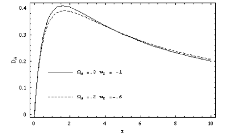
Figure 1: The angular diameter distance fortwo different FLRW universes. The unit of distance is taken to be $c/H_{0}$.

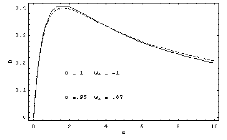
Figure 2: The angular diameter distance fordifferent values of $\alpha_{M}$ and $w_{X}$ ($\Omega_{M}$ is equal to 0.3). The unit of distance is taken to be$c/H_{0}$.

5 Parameter degeneration

As seen, the consideration of the DR equation in its full generality, with respect to the case of a homogeneous cosmological constant, demands the introduction of new parameters. Let us study the case of homogeneous dark energy ($\alpha_{X}=1$).

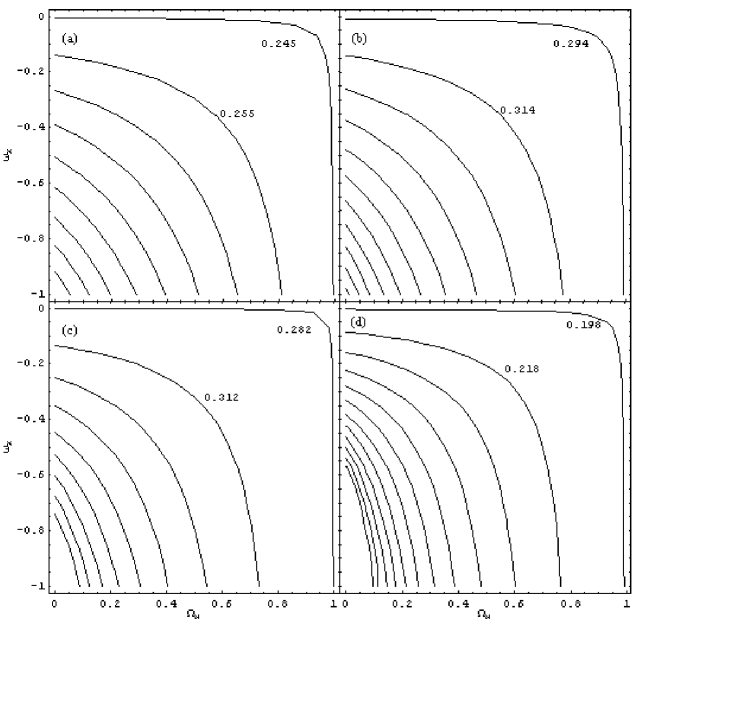
Figure 3: The angular diameter distance in the$\Omega_{M}-w_{X}$ plane, when $\alpha_{M}=\alpha_{X}=1$. The distance increases from the top-right to the bottom-left corner. a) We assume $z=0.5$; each contour is drawn with steps of 0.01. b) We assume $z=1$; the step is 0.02. c) We assume $z=2$; the step is 0.03. d) We assume $z=5$; the step is 0.02. The unit of distance is taken to be $c/H_{0}$.

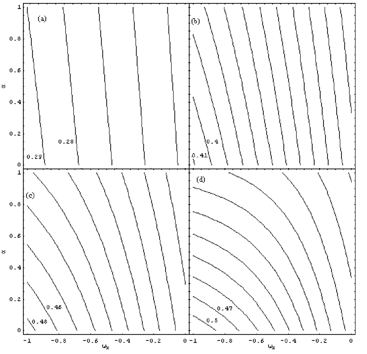
Figure 4: The angular diameter distance in the$w_{X}-\alpha_{M}$ plane, when $\Omega_{M}=1$ and $\alpha_{X}=1$. The distance increases from the top-right to the bottom-left corner. a) We assume $z=0.5$; each contour is drawn with steps of 0.01. b) We assume $z=1$; the step is 0.01. c) It is $z=2$; the step is 0.02. d) it is $z=5$; the step is 0.03. The unit of distance is taken to be $c/H_{0}$.

For $\alpha_{X}=1$, equation (54), in units of $c/H_{0}$, simplyfies to

$$D_{A}(z)=D_{1}(z)+\int_{0}^{z}\sum_{i=1}^{\infty}K_{i}(y,z)D_{1}(y)dy,$$ (62)

while equation (59) reduces, for $y\leq z$, to

$$K_{1}(y,z)=\frac{3}{2}(1-\alpha_{M})\Omega_{M}\frac{H_{0}}{H(y)}(1+y)^{2}D_{1}(y,z).$$ (63)

Some monotonical properties with respect to the cosmological parameters are then easily derived. For an accelerated universe ($w_{X}<-1/3$), it is

$$\frac{\partial}{\partial\Omega_{X}}\frac{1}{H(z)}>0,\ \frac{\partial}{\partial\Omega_{X}}D_{1}(z)>0\ {\rm if}\ w_{X}<-1/3,$$ (64)

and so, for every value of the clumpiness parameter $\alpha_{M}$, the angular diameter distance increases with increasing $\Omega_{X}$,

$$\frac{\partial}{\partial\Omega_{X}}D_{A}(z)>0\ {\rm if}\ w_{X}<-1/3.$$ (65)

When $w_{X}>-1/3$, the inequalities in equation (64) are reversed and the distance decreases with increasing $\Omega_{X}$. With respect to the equation of state $w_{X}$, it is

$$\frac{\partial}{\partial w_{X}}\frac{1}{H(z)}<0,\ \frac{\partial}{\partial w_{X}}D_{1}(z)<0;$$ (66)

and so

$$\frac{\partial}{\partial w_{X}}D_{A}(z)<0;$$ (67)

large values of the distances correspond to large negative values of the pressure of quintessence so that, for fixed $\Omega_{M}$, $\Omega_{X}$ and $\alpha_{M}$, the angular diameter distance takes its maximum when the dark energy is in the form of a cosmological constant.

We now want to stress the dependences of the angular diameter distance on $w_{X}$, $\Omega_{M}$ and $\alpha_{M}$ in flat universes with $\alpha_{X}=1$. As Fig.1 and Fig.2 show, the angular diameter distance is degenerate with respect to different pairs of parameters, since the distance in the $\Lambda$CDM model with $\Omega_{M}=0.3$ is not distinguishable, within the current experimental accuracy (Perlmutter et al. 1999), from the one in a FLRW universe with less pressureless matter but a greater value of $w_{X}$ or from an inhomogeneous universe with greater $w_{X}$ and the same content of matter.

In Fig.3, we plot the degenerate values of the distance in the $\Omega_{M}-w_{X}$ plane when universe is homogeneous for four different source redshifts: as expected, the dependence of the distance on the cosmological parameters increases with the redshift of the source. A general feature is that the distance is less sensitive to the components of the universe when $\Omega_{M}$ is near unity and $w_{X}$ goes to 0. This is easily explained: when $\Omega_{M}$ is large, quintessence density $\Omega_{X}$ is not, and the pressureless matter characterizes almost completely the universe; moreover, a value of $w_{X}$ near zero describes a dark energy with an equation of state very similar to that of the ordinary matter. So, increasing $w_{X}$ mimics a growth in $\Omega_{M}$. On the other side, for low values of $\Omega_{M}$ ($w_{X}$) the distance is very sensitive to $w_{X}$ ($\Omega_{M}$) and this effect increases with the redshift. We see from Fig.3 that the effects of $w_{X}$ and $\Omega_{M}$ are of the same order for a large range of redshifts.

In Fig.4 we compare, for $\Omega_{M}$ fixed to 0.3 and for different source redshifts, the compelling effects of $\alpha_{M}$ and $w_{X}$ on the distance. When $\alpha_{M}$ goes away from the usually assumed value ($\alpha_{M}=1$), once fixed the redshift, the distance increases; on the contrary, for $w_{X}$ that goes away from the value corrensponding to the cosmological constant ($w_{X}=-1$), the distance decreases. The dependence of the distance on $\alpha_{M}$ increases very rapidly with $z$, and, when $z=5$, the effects of $\alpha_{M}$ and $w_{X}$ are of the same order. From Fig.4 we deduce that the dependence on $\alpha_{M}$ increases when $w_{X}$ goes to $-1$, since values of $w_{X}$ near zero have the effect to smooth the universe. In fact, when $w_{X}=-1$, both a fraction $\alpha_{M}$ of the pressureless matter and of the cosmological constant are uniformly distributed; when $w_{X}\rightarrow 0$, quintessence behaves like ordinary matter, and so, for the same value of $\alpha_{M}$, the pressureless matter homogeneously distributed is $\alpha_{M}\Omega_{M}+\Omega_{X}=1-(1-\alpha_{M})\Omega_{M}$. Intermediate values of $w_{X}$ interpolate between these two extreme cases.

Figure 5: For flat homogeneous universes $z_{m}$is determined by the intercept between the angular diameter distance and the always decreasing Hubble distance. The values on the ordinate axis are in units of $c/H_{0}$. It is $\Omega_{M}=0.3,\ w_{X}=-1$.

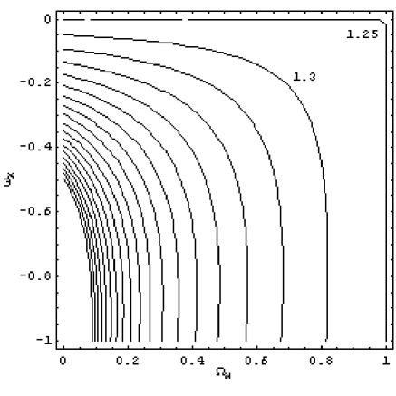
Figure 6: Contours of equal $z_{m}$ on the $\Omega_{M}-w_{X}$ plane for flat homogeneous universes. Each contour is drawn with a step of 0.05.

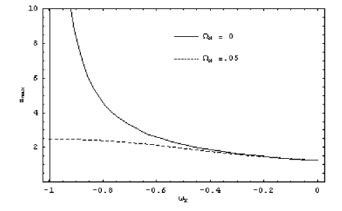
Figure 7: $z_{m}$ as a function of $w_{X}$ for two valuesof $\Omega_{M}$. For $\Omega_{M}=0.05$, $z_{m}$ nearly halves itself (from 2.47 to 1.25) when $w_{X}$ goes from $-1$ to $0$.

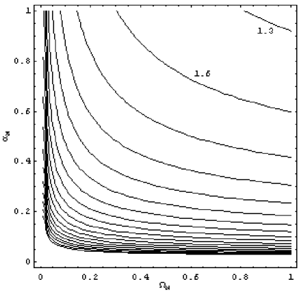
Figure 8: Contours of equal $z_{m}$ on the $\Omega_{M}-\alpha_{M}$plane for universes with a cosmological constant. Contours are drawn with steps of 0.03.

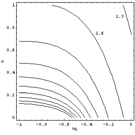
Figure 9: Contours of equal $z_{m}$ on the $w_{X}-\alpha_{M}$ plane for flat universes with $\Omega_{M}=0.3$ and $\alpha_{X}=1$. Contours are drawn with steps of 0.03.

6 The critical redshift

The critical redshift at which the angular diameter distance of an extragalactic source takes its maximum value has already been studied for the case of a flat $\Lambda$CDM universe by Krauss & Schramm [Krauss & Schramm1993] and for a flat universe with quintessence by Lima & Alcaniz [Lima & Alcaniz 2000]. In this section, we will find again their results with a new approach and will extend the analysis to inhomogeneous flat universes.

As can be seen cancelling out the derivative of the right hand of equation (28) with respect to $z$, the critical redshift $z_{m}$ for a flat homogeneous universe occurs when

$$D_{A}(z_{d},z_{m})=\frac{c}{H(z_{m})},$$ (68)

so that the angular diameter distance between an observer at $z=z_{d}$ and a source at $z_{m}$ is equal to the Hubble distance for $z=z_{m}$, as you can see in Fig.5. Equation (68) is an implicit relation that gives the dependence of $z_{m}$ on $z_{d},\Omega_{M}$ and $w_{X}$ . Throughout this section, we will put $z_{d}=0$. In Fig.6 we show $z_{m}$ for a homogeneous flat universe. For a given value of $w_{X}$ ($\Omega_{M}$), $z_{m}$ decreases with increasing $\Omega_{M}$ ($w_{X}$); when $\Omega_{M}=0$, $z_{m}$ diverges for $w_{X}=-1$, but also a small value of $\Omega_{M}$ is sufficient to eliminate this divergence (see Fig.7). The minimum value of $z_{m}$ corresponds to the Einstein-de Sitter universe ($\Omega_{M}=1$ or $w_{X}=0$), when $z_{m}=1.25$. As you can see from Fig.6, for values of $w_{X}$ in the range $(-1,-0.8)$, once fixed $\Omega_{M}$, $z_{m}$ is nearly constant and this trend increases with $\Omega_{M}$; on the contrary, for small $\Omega_{M}$ $(\stackrel{{\scriptstyle<}}{{\sim}}0.4)$ and $w_{X}\stackrel{{\scriptstyle>}}{{\sim}}-0.4$, $z_{m}$ is very sensitive to $w_{X}$. The small changes of $z_{m}$ in the region of large $\Omega_{M}$ and $w_{X}$ are explained with considerations analogous to those already made in the previous section for the values of the distance in the $\Omega_{M}-w_{X}$ plane.

Let us go now to analyse the effect of $\alpha_{M}$ on $z_{m}$. By differentiating equation (33) and equation (34) with respect to $z$, we see that the derivatives are zero only for $z\rightarrow\infty$: i.e., in flat universes with totally inhomogeneous quintessence or in a generic model with cosmological constant, the critical redshift is not finite when $\alpha_{M}=0$. So with respect to $z_{m}$, a totally clumpy universe, indipendently of $\Omega_{M}$ and $w_{X}$, behaves like a FLRW model completely dominated by the vacuum energy. In fact, the cosmological constant, differently from dark energy with $w_{X}>-1$, does not give contribution to the Ricci focusing and the same occurs for the pressureless matter with $\alpha_{M}=0$. In Fig.8 we show $z_{m}$ in the $\Omega_{M}-\alpha_{M}$ plane for $w_{X}$ fixed to $-1$. The critical redshift decreases with increasing $\Omega_{M}$ and $\alpha_{M}$, and takes its minimum for the Einstein-de Sitter universe $(\Omega_{M}=\alpha_{M}=1)$, that is when the focusing is maximum. On the other side, $z_{m}$ is very sensitive to $\alpha_{M}$, especially for large values of $\Omega_{M}$ since $\alpha_{M}$ appears in the DR equation as a multiplicative factor of $\Omega_{M}$. For $\Omega_{M}=0.3$, $z_{m}=1.61$ and 3.23 for, respectively, $\alpha_{M}=1$ and 0.2, a variation of 100%. So, combining different cosmological tests to constrain the other cosmological parameters, we can use the redshift-distance relation to guess the smoothness parameter $\alpha_{M}$ in a quite efficient way.

We conclude this section comparing the influence of $\alpha_{M}$ and $w_{X}$ on the critical redshift. Fig.9 displays $z_{m}$ in the $\alpha_{M}-w_{X}$ plane, for $\Omega_{M}$ fixed to 0.3 and with $\alpha_{X}=1$. As expected, $z_{m}$ increases when the focusing decreases, that is for small values of $\alpha_{M}$ and $w_{X}$. We can see that the effects of $\alpha_{M}$ and $\Omega_{M}$ are of the same order.

7 Conclusions

The question of light propagation in an inhomogeneous universe is an open topic of modern cosmology and the necessity of a positive solution grows up with the increasing means of experimental technology that begins to explore very high redshifts. In particular, the cosmological distances, which provide important probes of the universe, are very sensitive to cosmological inhomogeneities. In fact, in the present quite poor data samples, sources usually appear dimmer and smaller with respect to homogeneous models for the systematic effect of under-densities along the different lines of sight. Here, we have investigated the properties of the angular diameter distance in presence of either clumpy pressureless matter and inhomogeneous dark energy using the ’empty beam approximation’.

The equation for the angular diameter distance with respect to the redshift has been found in a way that is indipendent from the focusing equation. The multiple lens-plane theory allows to derive the DR equation for inhomogeneous quintessence, in a way that makes clear the importance of the ’empty beam approximation’ in the gravitational lensing.

We have given useful forms for the distance. For non flat universe, we have studied the case of cosmic string network, when the angular diameter distance is expressed in terms of hypergeometric functions, and an accelerated universe with $w_{X}=-2/3$ (domain walls), when the distance-redshift relation is given in terms of Heun functions. For the very interesting case of flat universes with inhomogeneous quintessence, we have obtained the solution of the DR equation in terms of hypergeometric functions. Then, we have listed the expressions for the distance when it takes the form of elementary functions for two particular cases of flat models: strictly homogeneous (we have considered cosmic string networks again) and totally inhomogeneous universes, i.e. both pressureless matter and dark energy solely in clumps.

As it could be reasonably expected, the angular diameter distance is degenerate, also considering a smooth quintessence, with respect to cosmological parameters: although there is a strong dependence both on the smoothness parameter $\alpha_{M}$ and the equation of state $w_{X}$, the intrinsic systematic errors prevent us to univocally determine the cosmological parameters only from measurements of distance. Nevertheless, combinig these data with indipendent observations like that concerning the cosmic microwave backgroung radiation, we can estimate the smoothness parameter $\alpha_{M}$ by determining the critical redshift, for example.

The effect of $w_{X}$ and $\alpha_{M}$, especially at high redshifts, are of the same order but very different. An increase in $w_{X}$ mimics a larger $\Omega_{M}$, while a more inhomogeneous universe (small $\alpha_{M}$) mimics the effect of a cosmological constant. This last statement agrees with what found by Célérier [Célérier 2000], in a very different context, that is by relaxing the hypothesis of large scale homogeneity for the universe. We have obtained a similar result by adopting the cosmological principle.

References

- [Caldwell et al. 1998] Caldwell R.R., Dave R., Steinhardt P.J., 1998, Phys. Rev. Lett. 80, 1582
- [Célérier 2000] Célérier M.N., 2000, A&A 353, 63
- [de Bernardis et al. 2000] de Bernardis P. et al., 2000, Nature 404, 955
- [ Demianski et al. 2000] Demianski M., de Ritis R., Marino A.A. & Piedipalumbo E., 2000, astro-ph/0004376
- [ Dyer & Roeder 1972] Dyer C.C., Roeder R.C., 1972, ApJ 174, L115
- [ Dyer & Roeder 1973] Dyer C.C., Roeder R.C., 1973, ApJ 180, L31
- [ Erdélyi et al. 1955] Erdélyi A., Magnus W., Oberhettinger F., Tricomi F.G., 1955, Higher Trascendental Functions Vol.3, McGraw Hill Book Company, New York
- [ Etherington 1933] Etherington I.M.H., 1933, Phil. Mag. 15, 761
- [ Giovi et al. 2000] Giovi F., Occhionero F., Amendola L., 2000, astro-ph/0011109
- [ Grishchuk 1994] Grishchuk L.P., 1994, Phys. Rev. D 50, 7154
- [ Gurvits et al. 1999] Gurvits L.I., Kellermann K.I., Frey S., 1999, A&A 342, 378
- [ Ince 1956] Ince E.L., 1956, Ordinary Differential Equations, Dover, New York
- [ Kantowski 1969] Kantowski R., 1969, ApJ 155, 89
- [ Kantowski 1998] Kantowski R., 1998, ApJ 507, 483
- [ Kantowski & Thomas 2000] Kantowski R., Thomas R.C., 2000, astro-ph/0011176
- [ Kantowski et al. 2000] Kantowski R., Kao J.K., Thomas R.C., 2000, astro-ph/0002334
- [ Krasiński 1997] Krasiński A., 1997, Inhomogeneous Cosmological Models, Cambridge University Press
- [Krauss & Schramm1993] Krauss L.M., Schramm D.N., 1993, ApJ 405, L43
- [ Lima & Alcaniz 2000] Lima J.A.S., Alcaniz J.S., 2000, A&A 357, 393
- [ Linder 1988] Linder E.V., 1988, A&A 206, 190
- [ Maor et al. 2000] Maor I., Brustein R., Steinhardt P.J., 2000, astro-ph/0007297
- [ Perlmutter et al. 1999] Perlmutter S. et al., 1999, ApJ 517, 565
- [ Picone & Miranda 1943] Picone M., Miranda C., 1943, Esercizi di analisi matematica, Studium Urbis, Roma
- [ Riess et al. 1998] Riess A.G. et al., 1998, ApJ 116, 1009
- [ Sachs 1961] Sachs R.K., 1961, Proc. Roy. Soc. London A 264, 309
- [ Schneider & Weiss 1988] Schneider P., Weiss A., 1988, ApJ 327, 526
- [ Schneider et al. 1992] Schneider P., Ehlers J., Falco E.E., 1992, Gravitational Lenses, Springer-Verlag, Berlin
- [ Seitz & Schneider 1994] Seitz S., Schneider P., 1994, A&A 287, 349
- [ Seitz at al. 1994] Seitz S., Schneider P., Ehlers J., 1994, Class. Quant. Grav. 11, 2345
- [ Silveira & Waga 1997] Silveira V., Waga I., 1997, Phys. Rev. D 56, 4625
- [ Spergel & Pen 1997] Spergel D., Pen U., 1997, ApJ 491, L67
- [ Turner & White 1997] Turner M.S., White M., 1997, Phys. Rev. D 56, 4439
- [ Tricomi 1985] Tricomi F.G., 1985, Integral Equations, Interscience Publishers, Inc., New York
- [ Vilenkin 1984] Vilenkin A., 1984, Phys. Rev. Lett 53, 1016
- [ Wang at al. 2000] Wang L., Caldwell R.R., Ostriker J.P., Steinhardt P.J., 2000, ApJ 530, 17
- [ Wang 1999] Wang Y., 1999, ApJ 525, 651
- [ Wang 2000] Wang Y., 2000, ApJ 536, 531
- [ Zel’dovich 1964] Zel’dovich Y.B., 1964, Soviet Ast. AJ 8, 13