New OH Zeeman measurements of magnetic field strengths in molecular clouds

Abstract

We present the results of a new survey of 23 molecular clouds for the Zeeman effect in OH undertaken with the ATNF Parkes 64-m radio telescope and the NRAO Green Bank 43-m radio telescope. The Zeeman effect was clearly detected in the cloud associated with the H II region RCW 38, with a field strength of $38\pm 3$ $\mu$G, and possibly detected in a cloud associated with the H II region RCW 57, with a field strength of $-203\pm 24$ $\mu$G. The remaining 21 measurements give formal upper limits to the magnetic field strength, with typical 1$\sigma$ sensitivities $<20$ $\mu$G.

For 22 of the molecular clouds we are also able to determine the column density of the gas in which we have made a sensitive search for the Zeeman effect. We combine these results with previous Zeeman studies of 29 molecular clouds, most of which were compiled by Crutcher (1999), for a comparsion of theoretical models with the data.

This comparison implies that if the clouds can be modeled as initially spherical with uniform magnetic fields and densities that evolve to their final equilibrium state assuming flux-freezing then the typical cloud is magnetically supercritical, as was found by Crutcher (1999). If the clouds can be modeled as highly flattened sheets threaded by uniform perpendicular fields, then the typical cloud is approximately magnetically critical, in agreement with Shu et al. (1999), but only if the true values of the field for the non-detections are close to the 3$\sigma$ upper limits. If instead these values are significantly lower (for example, similar to the 1$\sigma$ limits), then the typical cloud is generally magnetically supercritical.

When all observations of the Zeeman effect are considered, the single-dish detection rate of the OH Zeeman effect is relatively low. This result may be due to low mean field strengths, but a more realistic explanation may be significant field structure within the beam. As an example, for clouds associated with H II regions the molecular gas and magnetic field may be swept up into a thin shell, which results in a non-uniform field geometry and measurements of the beam-averaged field strength which are significantly lower than the true values. This effect makes it more difficult to distinguish magnetically subcritical and supercritical clouds.

1 Introduction

Magnetic fields are widely believed to influence the stability and dynamics of molecular clouds and to explain the supersonic line widths seen in all interstellar molecular spectral lines (see reviews by Heiles et al. 1993; McKee et al. 1993; and references therein). Yet these central ideas in molecular cloud and star formation physics are supported by remarkably few measurements of magnetic field strengths, due to the difficulty in measuring the Zeeman effect in molecular lines such as the 18 cm lines of OH. Excluding masers, for which the velocity dispersion and gas density are very uncertain, there are only 17 clouds in which the Zeeman effect has been detected above 3$\sigma$ (Crutcher 1999; Sarma et al. 2000; Crutcher & Troland 2000).

As discussed in detail in the reviews by Heiles et al. (1993) and Crutcher (1994), the only viable technique available for measuring magnetic field strengths in molecular clouds is the Zeeman effect in spectral lines. The magnetic field reveals itself via the Zeeman effect as small frequency shifts, $\Delta\nu_{z}$, in the right and left circularly polarized (RCP and LCP, respectively) components of the spectral line with respect to the frequency in the zero field case, $\nu_{\mathrm{o}}$. The magnetic field strength can be determined by measuring this frequency shift. However, under most astrophysical conditions $\Delta\nu_{z}\ll\Delta\nu$, where $\Delta\nu$ is the full width at half maximum of the spectral line (the exceptions are masers, see e.g., Reid & Silverstein 1990), and so detecting the shift between the RCP and LCP components due to the the Zeeman effect is difficult, and complete information about the magnetic field direction and magnitude is not obtainable. In this situation only the determination of the line-of-sight component of the field strength, $B_{los}$ (= $B\cos\theta$), and its sign (i.e., toward or away from the observer) is possible.

The most succussful efforts have been those of Crutcher and collaborators (e.g., Crutcher & Kazès 1983; Kazès & Crutcher 1986; Troland, Crutcher & Kazès 1986; Crutcher, Kazès & Troland 1987; Kazès et al. 1988, Goodman et al. 1989; Crutcher et al. 1993; Roberts, Crutcher & Troland 1995; Crutcher et al. 1999a), mainly through observations of the OH transitions at 1665 and 1667 MHz. Almost all successful detections of the Zeeman effect have used this technique, with observations of H I and CN also yielding success (e.g., Roberts et al. 1993; Brogan et al. 1999; Crutcher et al. 1999b). The major telescopes that have been used are Nançay (OH), the Hat Creek 85-ft (H I), the NRAO 43-m (OH, H I), Arecibo (OH, H I), the VLA (OH, H I), and the IRAM 30-m (CN).

All the reliable detections, and a number of upper limits were compiled by Crutcher (1999) for comparison with theory. In addition to the field strength or upper limit for each cloud in his analysis (27 clouds), Crutcher also compiled information on the column density, line width, number density, temperature and size for each molecular cloud. By comparing the data against a model spherical cloud with uniform density and uniform magnetic field, with corrections for the simple virial terms, Crutcher concluded that (i) internal motions are supersonic, (ii) the ratio of magnetic to thermal pressure is sufficient for magnetic fields to be important, (iii) the mass-to-magnetic flux ratio is about twice critical, which suggests that static magnetic fields alone may be insufficient to provide cloud support, (iv) the kinetic and magnetic energies are approximately equal, which implies that MHD waves and static fields are equally important in cloud dynamics, and (v) magnetic field strengths scale with gas densities in agreement with the predictions of ambipolar diffusion, $|B|\propto\rho^{0.47}$. However, we note that the scatter in this last result is significant, and it does not take into account measured upper limits to $B_{los}$.

Shu et al. (1999) compared the data of Crutcher (1999) with a model of a highly flattened molecular cloud (Allen & Shu 2000), and found that the mass-to-magnetic flux ratio is approximately critical. Considering the uncertainties in the measurements and the simple nature of the model, Shu et al. concluded that it could not yet be decided whether the clouds are generally magnetically subcritical (slow evolution, dominated by ambipolar diffusion) or supercritical (fast evolution, dominated by collapse and fragmentation), though the distinction is clearly very important.

Further, the role of the magnetic field in cloud support has been questioned since magneto-hydrodynamic (MHD) simulations indicate that unforced MHD turbulence decays in about a free-fall time (MacLow et al. 1998; Padoan & Nordland 1999; Stone, Ostriker & Gammie 1998), and since examination of stellar ages indicates that star-forming molecular clouds may not require long-lived support from either turbulence or magnetic fields (Elmegreen 2000, Hartmann 2001).

Since progress in this field clearly requires more observations, we have undertaken OH Zeeman observations of molecular clouds in the relatively unexplored southern hemisphere and observations of a sample of northern hemisphere molecular clouds not previously studied.

2 Observations

2.1 Parkes

OH Zeeman observations of southern hemisphere molecular clouds were undertaken in 1995 July and 1996 October with the Australia Telescope National Facility (ATNF) Parkes 64-m radiotelescope, using a HEMT receiver equipped with dual linear polarization feeds. This system provided cold-sky system temperatures of $T_{sys}$ $\sim$20-25 K. The OH ground state transitions at 1665.40184 (hereafter, the OH 1665 line) and 1667.35901 MHz (hereafter, the OH 1667 line) were observed simultaneously in one bandpass of 4 MHz centered on 1666 MHz with a channel separation of 488.28 Hz (0.087 km s^-1). The outputs from the linear feeds were crossed in a hybrid coupler located immediately after the low noise amplifiers of the receiver to produce right- and left-hand circular polarized outputs (RCP and LCP respectively). These signals were then passed through a double-pole, double-throw polarization switch to minimize the effects of instrument polarization and gain differences on the spectra, switching every $\sim$10 seconds. The center bandpass frequency was switched by $\pm$0.25 MHz every 4 minutes. Both senses of circular polarization were observed and recorded simultaneously. The FWHM beam size at these frequencies is $\sim$13′ and the main beam efficiency is $\sim$0.7.

To determine the sense of polarization in the output from the correlator, OH masers having strong circular polarization were observed at the start of each run (Caswell et al. 1980; Caswell & Haynes 1983, 1987a). We used Zeeman observations of the deep OH absorption line toward Orion B to test our setup. In both observing periods we were able to reproduce the results of Crutcher & Kazès (1983; hereafter CK83) after $\sim$5 hr integration time. By combining the 1665 and 1667 OH results from 1995 and 1996 a field strength of $35\pm 2$ $\mu$G is inferred for the subcomponent identified by CK83 as the source of the Zeeman pattern, essentially independent of hour angle. The Stokes $I$ and $V$ spectra for Orion B observed in 1996 are shown in Figure New OH Zeeman measurements of magnetic field strengths in molecular clouds. These values are in agreement with the value determined by CK83 ($38\pm 1$ $\mu$G) using the Nançay telescope. It should be noted that the magnetic field strength inferred for Orion B is not unique, but depends on the properties (line strength, line width) of the subcomponent, which are not fully constrained by the observations.

The displacement of the right- and left-circularly polarized beams on the sky, commonly called “beam-squint” (e.g., Troland & Heiles 1982) can result in a spurious Zeeman effect if there exists a sufficiently large component of velocity gradient in the spectral line along the same direction as the squint. This effect is diminished considerably with the combination of an altitude-azimuth telescope such as Parkes and a long on-source integration time, since the source then rotates within the beam and the true Zeeman signal is modulated. For Parkes we measured a squint of $\sim$15″ for both observing runs, but with different position angles, most likely caused by the replacement of the focus cabin at the end of 1995. While this is a relatively large value for the squint, the fact that we were able to reproduce the results for Orion B both times with the same derived magnetic field strength suggests that the squint is not a problem for our observations. If a spurious Zeeman effect had been caused by squint then the inferred magnetic field strength for the OH 1665 line would be 1.7 times greater than the OH 1667 line, which we do not see in our results.

2.2 Green Bank

OH Zeeman observations of northern hemisphere molecular clouds were undertaken in 1996 September and 1998 June with the National Radio Astronomy Observatory (NRAO) Green Bank 43-m telescope, using a dual channel cooled HEMT receiver with circular polarization feeds. Cold sky system temperatures of 20–25 K were recorded with this system. The OH 1665 and 1667 MHz lines were observed simultaneously in both polarizations with frequency switching with a channel separation of 1220 Hz ($\sim$0.22 km s^-1). To minimize the effect of instrument polarization and gain differences on the spectra polarization switching was performed at a rate of $\sim$1 Hz. The setup is similar to the one used by Crutcher et al. (1993). The FWHM beam size at these frequencies is $\sim$18′ and the main beam efficiency is $\sim$0.7.

As was the case for the Parkes observations, we tested the setup with OH Zeeman observations of Orion B. The Zeeman effect was clearly seen during both observing sessions, and by combining the 1665 and 1667 OH results for 1996 and 1998 we infer a magnetic field strengths of $34\pm 3$ $\mu$G for the subcomponent identified by CK83.

We measured the beam squint of the 43-m telescope to be no more than 1″. Beam squint is more important for an equatorially mounted telescope such as the 43-m compared to an alt-az telescope, if the squint happens to align with a velocity gradient within the source being observed. However, the chances of such an alignment are small, and the change in hour angle will not cause any change in alignment between the squint and velocity gradient.

2.3 Mopra Observations

As OH and ¹³CO are believed to trace similar column densities (e.g., Myers et al. 1978; Heiles et al. 1993), we have mapped a number of the southern clouds (those observed at Parkes) in the ¹³CO $J=1\rightarrow 0$ transition, in order to provide an independent measurement of the column density, and to resolve more structure than is possible with the poor angular resolution provided by the OH observations. The observations were undertaken in April 1997 with the 22-m ATNF Mopra radiotelescope. At the ¹³CO $J=1\rightarrow 0$ frequency of 110201.37 MHz only the inner 15-m of the surface was illuminated at the time of our observations, providing an effective beam size of 45″. The receiver was a dual linear polarization SIS receiver with a total system temperature measured to be $\sim$150 K in good weather. The 16384 channel autocorrelator was configured for two IFs, providing a spacing between channels of 0.17 km s^-1 over a velocity range of $\sim$220 km s^-1 (1024 spectral channels with a 64 MHz bandwidth) at the ¹³CO $J=1\rightarrow 0$ frequency. One IF was centered on the ¹³CO $J=1\rightarrow 0$ frequency, the second being centered on the SiO $\nu$ = 1, $J=2\rightarrow 1$ transition at 86243.44 MHz for regular pointing checks using SiO masers listed in the SEST Handbook (http://www.ls.eso.org/lasilla/Telescopes/SEST/SEST.html).

The mapping was performed on a 1′ grid in position switching mode, with an on-source integration time of 4 minutes per position. Removal of first-order baselines was sufficient in most cases to correct for any system effects not removed by the reference observation. The spectra were calibrated offline for atmospheric attenuation and the variation of telescope beam efficiency with elevation, and the intensity scaled to the $T_{A}^{*}$ scale of SEST by observations of Orion ($\alpha_{1950}=05^{\rm h}32^{\rm m}47\fs 0$, $\delta_{1950}=-05\arcdeg 24\arcmin 23\arcsec$) in the ¹³CO $J=1\rightarrow 0$ transition, assuming $T_{A}^{*}$(Orion) = 13 K (Appendix of the SEST Handbook). The conversion to $T_{mb}$ is given by $T_{mb}$ = $T_{A}^{*}$/$\eta_{mb}^{\mathrm{S}EST}$ where $\eta_{mb}^{\mathrm{S}EST}$ = 0.7 near 110 GHz. In general we attempted to map down to at least the 50% level of the peak emission in each source.

3 Source Selection

3.1 Southern sources

Our initial search for suitable sources centered on the OH studies of Robinson, Goss & Manchester (1970), Goss, Manchester & Robinson (1970), Manchester, Robinson & Goss (1970), Robinson, Caswell & Goss (1971), Caswell & Robinson (1974), and Turner (1979). The spectral resolution of these previous observations, many undertaken with Parkes, was generally insufficient to detect weak, narrow maser features, and so we reobserved all our potential targets with the setup described here. We also reobserved a number of other sources from these lists with a greater velocity coverage, as well as some sources from Dickel & Wall (1974), Toriseva, Höglund & Mattila (1985), and Chan, Henning & Schreyer (1996). None of the sources we surveyed from these lists showed any significant OH absorption that was not previously known.

In order to select suitable Zeeman candidates we required observations with substantial improvements in sensitivity and spectral resolution over the earlier OH surveys of southern HII regions. We thus re-observed $\sim$80 sources drawn from these lists to assess their suitability. To determine our primary candidates we used the “sensitivity estimator” given by Troland (1990; see also Goodman 1989) to estimate the integration time required per source to reach our target sensitivity of 3$\sigma$ $\sim$30 $\mu$G. In order to have the greatest sensitivity to the Zeeman effect, the spectral line profiles of the selected sources should be narrow and strong against a weak continuum source (so that the system temperature is as low as possible), and free of maser emission. Using these criteria we chose the 9 sources for our primary candidate list, selecting those sources with the lowest integration times required to reach the target sensitivity.

Previously unreported masers discovered in the survey are discussed in Appendix B.

3.2 Northern sources

Crutcher and co-workers have previously observed the most promising OH Zeeman candidates in the northern sky (Crutcher 1999). However, a number of promising sources remain to be studied. The best list to date is the extensive survey of OH by Turner (1979) using the NRAO 43-m telescope. Two of the previous detections of the Zeeman effect, S88B (Crutcher et al. 1987) and S106 (Kazès et al. 1988), have only modest OH line absorption depths of $T_{A}^{*}$ $\sim$ 0.5 as observed with the 43-m, but they are among the few sources with clearly detected Zeeman patterns. The Turner catalog contains a number of sources with similar line absorption depths. To select sources for Zeeman observations with the 43-m, we re-observed a number of candidates from the Turner catalog, as well as sources identified as H II regions from the IRAS database, sensitive continuum surveys, and water maser surveys (e.g., Chan et al. 1996; Carpenter, Snell & Schoerb 1990; Wouterloot, Brand & Fiegle 1993; Wouterloot & Brand 1989). We observed $\sim$200 sources, and identified 11 Zeeman candidates using the same criteria as for the Parkes sample.

The final source list is given in Table 1. Column 1 lists the source name, columns 2–3 the source position, and columns 4–6 the results of fitting a Gaussian to the OH 1667 line profile. Column 7 lists the continuum source temperature, where appropriate, and column 8 list the total on-source integration time for the Zeeman observations.

4 Results & Analysis

In Zeeman experiments, the magnetic field reveals itself as frequency shifts in the right and left circular polarized components ($I_{RCP}$ and $I_{LCP}$, respectively) of the spectral line. A full treatment of the Zeeman effect under astrophysical conditions may be found in Sault et al. (1990; see also Heiles et al. 1993), and we include only a brief discussion of the analysis here. In the situation where the frequency shift is much smaller than the line width (which is always the case for non-maser lines), the difference or Stokes $V$ spectrum, $V=I_{RCP}-I_{LCP}$, is only sensitive to the line-of-sight component of the magnetic field and can be modeled as

$$V=\frac{b}{2}B{\rm cos}\theta\frac{dI}{d\nu}+\beta I~{}~{},$$ (1)

where $b$ is the “Zeeman factor” and equals 3.27 and 1.96 Hz $\mu$G^-1 respectively for the 1665 and 1667 MHz lines of OH, $B$ is the magnetic field strength, $\theta$ is the angle between the field lines and the line-of-sight, $\beta$ is the “gain term” arising from gain differences between the RCP and LCP signal paths (Sault et al. 1990) and $I$ is the Stokes $I$ spectrum (=$I_{RCP}+I_{LCP}$). The Zeeman term in equation (1), $(b/2)B{\rm cos}\theta(dI/d\nu)$, reveals itself in the $V$ spectrum as the characteristic sideways “S”, or “Zeeman pattern”. The line-of-sight field strength $\mbox{$B_{los}$}=B{\rm cos}\theta$ is inferred from equation (1) by least-squares fitting the right hand side of this equation to the observed $V$ spectrum. Other fitting techniques are discussed and analysed in Sault et al. (1990).

4.1 Fitting $dI/d\nu$ to $V$

In Table 2 we present the results of our Zeeman analysis. In this Table column 1 lists the source name, column 2 the velocity of the OH feature, column 3 the magnetic field strength determined from the OH 1665 transition with its one sigma uncertainty, column 4 as for column 3 but for the OH 1667 transition, and column 5 the weighted mean line-of-sight field strength $B_{los}$ (found by combining the results for the 1665 & 1667 lines) and its weighted one sigma uncertainty $\sigma_{B}$ obtained by standard error analysis.

In the majority of sources the line profiles are simple and well fitted by a single Gaussian profile. Notable exceptions are RCW 38, RCW 57, W7, and G10.2-0.3. In these cases, alternative approaches to performing the Zeeman analysis are described in CK83, or Heiles (1988) and Goodman & Heiles (1994). In the method of CK83, the $V$ spectrum shows a clear “S” structure signifying the Zeeman effect, but it is too narrow to arise from the entire $I$ line profile. By integrating the $V$ spectrum and fitting the result with a Gaussian it is possible to infer the properties ($V_{lsr}$, $\Delta V$) of the component of the $I$ spectrum responsible for the “S”. The reality of such a component is strengthened if the same properties are derived for both the OH 1665 and 1667 lines. CK83 applied this method to Orion B (see Fig. New OH Zeeman measurements of magnetic field strengths in molecular clouds), and we have successfully used this technique to analyse RCW 38 (see below). In Heiles (1988) and Goodman & Heiles (1994) the $I$ profile is broken down into independent Gaussian subcomponents, and the $V$ spectrum is then modeled as the sum of derivatives of these components, with unique values of $B_{los}$ assigned to each component. We have applied this method to those sources for which a single Gaussian could not adequately be fitted to the $I$ spectrum and where the CK83 method is inappropriate, because there is no clear “S” in the $V$ spectra. These are indicated in the notes to Table 2. For G10.2–0.3, we were unable to fit a consistent set of Gaussians to the OH 1665 and 1667 lines.

In order for the derived magnetic field strength $B_{los}$ to be considered as a detection we require that the field strengths measured in both OH lines be consistent with each other, $\mid B_{1665}-B_{1667}\mid$ $<$ $\sigma_{B}$, and the field strength be greater than 3$\sigma_{B}$, $\mid B_{los}\mid$ $>$ 3$\sigma_{B}$. Only 2 sources, RCW 38 and RCW 57, can be considered as detections using these criteria. These are discussed below. We consider the remaining 21 measurements to give upper limits to $B_{los}$ averaged over our 13′ (Parkes) and 18′ (Green Bank) beams (see also §5.1).

Details of other properties for the individual sources, such as column densities, are given in Appendix A (see also Table 3).

4.2 Determination of Column Densities

The intensity of a spectral line from a uniform medium in front of a background region may be expressed as

$$T_{mb}=f[J(T_{ex})-J(T_{C})][1-\exp(-\tau)]~{}~{},$$ (2)

where $T_{mb}$ is the main-beam brightness temperature, $\tau$ is the optical depth of the cloud in the molecular transition, $f$ is the beam filling factor, $T_{ex}$ is the excitation temperature of the transition, $T_{C}$ is the area-weighted mean background temperature (the cosmic background temperature $T_{bg}$ plus any contribution from a background continuum source, $T_{S}$), and $J(T)=(h\nu/k)/(\exp(h\nu/kT)-1)$ is the Planck function. For sources observed in absorption against a compact continuum source, $f$ represents the fraction of the beam area covered by the continuum source. At the frequencies of the OH ground state transitions near 1.6 GHz $J(T)\equiv T$ for the temperatures observed in molecular clouds ($T\lesssim 100$ K), and so

$$T_{mb}=f[T_{ex}-T_{C}][1-\exp(-\tau)]~{}~{}.$$ (3)

The observed antenna temperature $T_{A}^{*}$ is proportional to $T_{mb}$, with a proportionality constant $\eta_{mb}$ (the main beam efficiency). With this knowledge it is possible to determine the column density of OH, $N(\mathrm{OH})$, which is given by (Goss 1968; Turner & Heiles 1971)

$$N(\mathrm{OH})=\frac{8\pi k\nu}{hc^{2}A}\mbox{$T_{ex}$}\ \frac{\sum g_{i}}{g_{u}}\int\tau d\nu~{}~{},$$ (4)

where $\nu$ is the frequency of the transition and $A$ is its Einstein A coefficient, $g_{i}$ is the statistical weight for level $i$ and $g_{u}$ is the statistical weight for the upper state of the transition. Thus, for the OH 1667 line

$$N(\mathrm{OH})=2.25\times 10^{14}\left(\frac{\mbox{$T_{ex}$}(1667)}{\mathrm{K}}\right)\tau_{1667}\left(\frac{\mbox{$\Delta v$}}{\mbox{km s${}^{-1}$}}\right)\mbox{cm${}^{-2}$}\ \,\,.$$ (5)

For clouds unassociated with H II regions, previous observations have shown that $T_{ex}$ is generally about 6 K (e.g., Turner 1973; Crutcher 1977, 1979), and we assume this value here. Clouds associated with H II regions are warmer, and so we assume $T_{ex}$ = 10 K for those clouds. For a cloud seen in absorption against a typical H II region $T_{C}\gg\mbox{$T_{ex}$}$ and $T_{ex}$ drops out of equation (3). We measure the product $fT_{C}$ at the telescope as $T_{sys}$(on-source) – $T_{sys}$(off-source), and the optical depth is then determined from equation (3), and the column density from equation (5). To determine the molecular hydrogen column density we assume a standard OH abundance ratio of [H]/[OH] = $2.5\times 10^{7}$ (Crutcher 1979), which is uncertain by about a factor two. High-angular resolution observations indicate that the OH abundance in unshocked gas found in PDRs associated with H II regions could be enhanced by as much as a factor of 5 over this value (Roberts et al. 1995; Sarma et al. 2000). Comparison of the data for NGC 6334 in Table 3 suggests that this is not a concern for the single-dish observations. Sarma et al. (2000) use an OH abundance five times greater than the dark cloud value and determine $N$(H₂) $\sim$ $5\times 10^{22}$ cm^-2, whereas we find $N$(H₂) $\sim$ $2\times 10^{22}$ cm^-2. The discrepancy would be greater if we used the same abundance as Sarma et al. (2000). Further support for the OH abundance ratio we use is given below.

Where it is possible to estimate the ¹³CO column density independently, or it has been previously determined (see appendix for individual cases), the values of the molecular hydrogen column density derived independently from OH and ¹³CO generally agree to within a factor two. For sources where a map of the ¹³CO emission exist, the line profile of ¹³CO averaged over the map is remarkable similar to OH, with similar line velocities (Fig. New OH Zeeman measurements of magnetic field strengths in molecular clouds). The agreement in line profile and the molecular hydrogen column density derived from ¹³CO and OH observations supports the assumption that these molecules trace similar physical conditions and the values for $T_{ex}$ and [H]/[OH] used here.

4.3 RCW 38

The Stokes $I$ and $V$ spectra for RCW 38 are shown in Figure New OH Zeeman measurements of magnetic field strengths in molecular clouds. The characteristic “S” shape of the Zeeman effect is clearly evident in the $V$ spectra, but is not well fitted by a scaled version of $dI/d\nu$. As discussed above, this suggests that the observed Zeeman profile is not due to the entire $I$ profile. The Zeeman profile is due to a subcomponent of the observed line, and we integrated the $V$ spectra to determine its properties. The integrated $V$ spectra are well fitted by single Gaussians, essentially with identical properties for the OH 1665 and 1667 lines. The line velocity and width for this component is given Table 2. From the fit of the derivative of this Gaussian to the OH lines we infer a value for the magnetic field of $B_{los}$ = $38\pm 3$ $\mu$G.

RCW 38 was observed during both observing sessions at Parkes. The results are consistent with each other. This helps to validate our result as a true Zeeman detection, as the direction of beam squint for the two observing sessions was different, even though the magnitude of the squint was large for Zeeman observations. In addition, no velocity gradients are apparent in a map of the OH absorption made during the 1996 observations. Corroborating evidence for the reality of the RCW 38 Zeeman detection comes from high angular resolution interferometric observations of the OH absorption made with the ATNF Compact Array (Bourke et al. 2001 in prep.). These observations indicate a compact, spatially isolated absorption feature with line velocity and width similar to those of the sub-component we infer as giving rise to the Zeeman effect.

RCW 38 is a bright H II region which has recently been observed in the near-infrared with the VLT (Alves et al. 2001 in prep). In a separate paper we present a detailed molecular line and continuum study of the region (Bourke et al. 2001 in prep.) which indicates that the Zeeman effect arises from a molecular clump on the western edge of the H II region, possibly associated with the bright 10 µm peak IRS1 (Smith et al. 1999). Assuming $T_{ex}$ = 10 K we determine $\tau_{1667}$ = 0.15, $N$(OH) = $7.6\times 10^{14}$ cm^-2, and $N$(H₂) = $9.3\times 10^{21}$ cm^-2. ¹³CO $J=1\rightarrow 0$ observations imply $N$(H₂) = $4\times 10^{21}$ cm^-2 (assuming [H₂]/[¹³CO] = $7\times 10^{5}$), lower than derived from the OH observations, which may suggest that the OH is sampling denser gas (e.g., Roberts et al. 1995 for S106). Observations of CS $J=2\rightarrow 1$ and C¹⁸O $J=1\rightarrow 0$ support this view (Bourke et al. 2001 in prep.).

4.4 RCW 57

The Stokes $I$ and $V$ spectra for RCW 57 are shown in Figure New OH Zeeman measurements of magnetic field strengths in molecular clouds. The $I$ profile is well fitted by two overlapping Gaussians, a deep absorption component at $V_{lsr}$ = –26.1 km s^-1 and a weaker component at $V_{lsr}$ = –22.6 km s^-1. The ¹³CO $J=1\rightarrow 0$ channel maps shown in Figure New OH Zeeman measurements of magnetic field strengths in molecular clouds reveal two spatially distinct clouds. The cloud in the north-east corresponds in velocity to the blue-shifted OH component, and the larger cloud to the south-west to the red-shifted OH component, which is the component for which we claim the detection of the Zeeman effect. The sum of ¹³CO emission spectra over the mapped region is remarkably similar to the OH absorption spectra (Fig. New OH Zeeman measurements of magnetic field strengths in molecular clouds), and is well fitted by two Gaussians with similar line velocities and widths as those fitted to the OH spectra.

The formal results for RCW 57 indicate a solid detection of the Zeeman effect in the $-22.6$ km s^-1 component, with $B_{los}$ = $-203\pm 24$ $\mu$G. However, inspection of the $V$ spectra in Figure New OH Zeeman measurements of magnetic field strengths in molecular clouds raises some doubt about this result. The blending of the two components makes it difficult to say with certainty that the Zeeman effect has been detected. At velocities greater than about $-22.2$ km s^-1 there is no overlap between the OH velocity components, and the Zeeman effect is clearly seen, but only part of the “S” is evident, due to the line overlap at lower velocities. As the ¹³CO observations show two spatially distinct clouds, follow-up OH Zeeman observations with the ATNF Compact Array should be able to resolve this question.

Located at a distance of 3.6 kpc (kinematic, e.g., Caswell & Haynes 1987b) or 2.4 kpc (Persi et al. 1994, based on the possible association of HD 97499 with the molecular cloud), RCW 57 (NGC 3576) is an H II region with ongoing star formation (e.g., Persi et al. 1994). The few published studies of this region suggest it is a “typical” H II region with associated molecular clouds. Whiteoak & Gardner (1974), observed the 5 GHz transition of H₂CO in absorption toward RCW 57 with a 4$\farcm$2 beam, and found two velocity components with almost identical properties to the Gaussian components we fitted to our OH data, suggesting that at least part of the OH absorption arises in somewhat denser gas (10⁴ cm^-3) than is usually sampled by OH (10³ cm^-3). For the component at –22.6 km s^-1 we find $\tau_{1667}$ = 0.06 and $N$(OH) = $8.9\times 10^{14}$ cm^-2, or $N$(H₂) = $1.1\times 10^{22}$ cm^-2 compared with $N$(H₂) = $1.3\times 10^{22}$ cm^-2 from ¹³CO Mopra observations. This is the component where we have a probable detection of the Zeeman effect, with $B_{los}$ = $-203\pm 24$ $\mu$G. For the component at –26.1 km s^-1 we find $\tau_{1667}$ = 0.2 and $N$(OH) = $1.5\times 10^{15}$ cm^-2, or $N$(H₂) = $1.9\times 10^{22}$ cm^-2 compared with $N$(H₂) = $1.5\times 10^{22}$ cm^-2 from ¹³CO Mopra observations.

5 Discussion

Of the 23 Gaussian components we could identify along the line-of-sight toward the 20 sources observed, the Zeeman effect was clearly detected in one source (RCW 38) and possibly in one component of another (RCW 57), as indicated in Table 2. In Table 2 we label our 23 components as those directly associated with H II regions (those clouds whose OH absorption line velocities are similar to the recombination line velocity of the background H II region) and those associated with (cold) molecular clouds along the line-of-sight. We find that 2 of 13 components associated with H II regions are detected, while none of the 10 components associated with cold molecular clouds are detected. The median 1$\sigma$ sensitivities for the H II and cold-cloud samples are respectively 11 and 9 $\mu$G.

A comparison of OH optical depth against line width shows no clear trend, nor does a comparison of integrated OH line area against optical depth. The molecular clouds showing Zeeman detections do not have properties clearly different to the other clouds in our sample.

5.1 The magnetic field and virial equilibrium

If the gas is well coupled to the magnetic field, then the large scale magnetic field can provide support against gravitational collapse. An important parameter in the discussion of support from large scale magnetic fields is the magnetic flux-to-mass ratio, $\Phi/M$. To examine whether this large scale field alone can provide support to molecular clouds, we ignore terms in the virial theorem other than the magnetic ($\mathcal{M}$) and gravitational ($\mathcal{W}$) energies, and assume that these energies are in equilibrium. This allows us to determine a critical mass, $M_{\rm cr}$, when gravitational forces are balanced by magnetic stresses (this has been discussed in detail in McKee et al. (1993); see also McKee 1999). It is found that $\mathcal{M}$ = $\mathcal{W}$ implies

$$M_{\rm cr}=\frac{c_{\Phi}\Phi}{\sqrt{G}}$$ (6)

where $G$ is the gravitational constant, and $c_{\Phi}$ is a numerical factor which depends on the geometry under consideration. For a spherical “parent” cloud with uniform density and uniform magnetic field, $c_{\Phi}$ $\approx$ 0.12 (Mouschovias & Spitzer 1976; Tomisaka, Ikeuchi & Nakamura 1988) for the final equilibrium configuration, which is flattened along the field lines (assuming flux-freezing). If the cloud is an isothermal disk (i.e., sheet-like) with a constant flux-to-mass ratio (uniform field and uniform column density), then $c_{\Phi}$ = 1/2$\pi\approx 0.16$ (Nakano & Nakamura 1978; Shu et al. 1999).

The critical mass can be related to observable quantities with measurements of the magnetic field strength $B$ and column density $N$ (McKee et al. 1993; Crutcher 1999), so that

$$\frac{\Phi}{M}=\frac{B}{mN}$$ (7)

where $m$ is the mean particle mass (2.33$m_{\rm H}$ for 10% He). The column density in equation (7) is the total column density, $N=1.2\mbox{$N$(H${}_{2}$)}$, for 10% He. The magnetic field strength is the total field strength, whereas Zeeman experiments where the Zeeman shift is less than a line width are only sensitive to the field along the line-of-sight, and hence measure $B_{los}$. As discussed in Crutcher (1999), we can statistically estimate the line-of-sight field strength for a large ensemble of measurements of uniform fields oriented randomly with-respect-to the line-of-sight, with the result that $<\mbox{$B_{los}$}>$ = $\mid B\mid$/2 and $<\mbox{$B_{los}$}^{2}>$ = $\mid B\mid$²/3. In addition, for the sheet-like geometry a correction factor to the observed column density is required, again due to the orientation with-respect-to the line-of-sight. In particular, if the magnetic field is preferentially perpendicular to the sheet, then the correction factors to the observed column density $N_{obs}$ and $B_{los}$ are not independent. Following the same argument as for the ensemble of magnetic field measurements given above, we find that $B/N$ = ($B_{los}$/$N_{obs}$)(cos${}^{2}\theta$) for one line-of-sight, so that $B/N$ = $<3\mbox{$B_{los}$}/N_{obs}>$ for the average over a distribution of equally likely line-of-sight directions. In terms of the critical magnetic flux-to-mass ratio,

$$\left(\frac{\Phi}{M}\right)_{\rm n}=\frac{\Phi}{M}\Bigg{/}\left(\frac{\Phi}{M}\right)_{\rm cr} = \frac{B}{mN}\left(\frac{\sqrt{G}}{c_{\Phi}}\right)^{-1}$$ (8)

$$= \digamma\,\frac{\mbox{$B_{los}$}}{2.8m_{\rm H}\mbox{$N$(H${}_{2}$)}}\left(\frac{\sqrt{G}}{c_{\Phi}}\right)^{-1}$$

where the subscript “n” indicates that the values of $\Phi/M$ have been normalized by the critical value $(\Phi/M)_{\rm cr}$, and $\digamma$ is the geometric correction factor, which is 2 for the initially uniform sphere, and 3 for the isothermal sheet. Evaluating the constants leads to

$$\left(\frac{\Phi}{M}\right)_{\rm n} = 2\times 10^{20}\frac{\mbox{$B_{los}$}}{\mbox{$N$(H${}_{2}$)}}\,\,{\rm cm^{2}\;\mbox{$\mu$G}}~{}~{}{\rm(sphere)}$$ (9)

$$= 4\times 10^{20}\frac{\mbox{$B_{los}$}}{\mbox{$N$(H${}_{2}$)}}\,\,{\rm cm^{2}\;\mbox{$\mu$G}}~{}~{}{\rm(sheet)}\,\,.$$ (10)

The values of ($\Phi/M$)_n for the different geometries considered above are given in Table 3. In this Table we also include the data for $B$ and $N$ compiled by Crutcher (1999) and recent Zeeman results from Sarma et al. (2000; NGC 6334) and Crutcher & Troland (2000; L1544). Therefore we believe Table 3 gives the most complete summary available of Zeeman measurements in extended molecular clouds (excluding small-scale OH maser emission). In column 1 is the source name, columns 2 & 3 give the line-of-sight field strength $B_{los}$ and its log, and column 4 lists the log of the molecular hydrogen column density. Column 5 lists the values of ($\Phi/M$)_n assuming an initially uniform sphere. Column 6 lists the values of ($\Phi/M$)_n assuming a sheet-like geometry. The values in Table 3 are shown graphically in Figure New OH Zeeman measurements of magnetic field strengths in molecular clouds. In this figure are plotted the measured field strength $B_{los}$ against the molecular hydrogen column density $N$(H₂), and overlayed with loci of ($\Phi/M$)_n for the uniform sphere model (a) and the sheet-like model (b).

Considering the values listed in Table 3 and plotted in Figure New OH Zeeman measurements of magnetic field strengths in molecular clouds, the results for the spherical parent cloud model are consistent with the clouds being slightly magnetically supercritical (($\Phi/M$)_n $<$ 1), the same result as found by Crutcher (1999), who only considered the detections he tabulated. The addition of our large number of upper limit measurements to his sample strongly reinforces this result. As noted by Crutcher (1999), assuming an initially uniform spherical cloud with a uniform magnetic field may be an oversimplification. In particular, if clouds are supported primarily by static magnetic fields with uniform direction they will become flattened as matter flows inward along field lines, and the field will become pinched along the direction perpendicular to the initial field direction. Therefore, the results for the sheet-like cloud may be more realistic. Considering only those clouds where the Zeeman effect was detected, Table 3 shows that the results for this geometry are consistent with ($\Phi/M$)_n $\approx$ 1, and the clouds are in approximate equilibrium between magnetic pressure and gravity, the same result found by Shu et al. (1999), though they did not distinguish between the detections and the upper limits. Because of the statistical corrections applied to $B$ and $N$, and the uncertainties in measuring $N$, a more definitive conclusion cannot be reached at present.

If we assume for the clouds where the Zeeman effect was not detected that the true magnetic field strengths are equal to the 3$\sigma$ upper limit values (listed in Table 3), then for the sheet-like model the mean flux-to-mass ratio is $<$($\Phi/M$)_n$>$ = $1.3\pm 0.9$ $\approx$ 1 (excluding G20.8–0.1 and G29.9+0.0 as the sensitivity of these observations is significantly less than the other data), the same results as for the detections. If the magnetic field within the beam is uniform, the true values are not likely to be greater than 3$\sigma$ for any of the clouds. On Figure New OH Zeeman measurements of magnetic field strengths in molecular clouds we also indicate the 1$\sigma$ limits for the non-detections. Assuming a uniform field, if the true field strengths are closer to the 1$\sigma$ limits than to the 3$\sigma$ limits then for the sheet-like model the mean flux-to-mass ratio is $<$($\Phi/M$)_n$>$ = $0.4\pm 0.3$, significantly lower than the critical value, which implies that in general the clouds are magnetically supercritical by a factor 2-3. As discussed below, field structure within the beam could reduce the flux-to-mass ratio by a factor 3–4 over its true value. However, beam dilution will also result in measurements of the column density lower than the true value for the gas in which the magnetic field is studied, which will increase the flux-to-mass ratio.

It is important to note that a number of the sources located at the upper end of Figure New OH Zeeman measurements of magnetic field strengths in molecular clouds (log $N$(H₂) $>$ 22.6) are due to high angular resolution VLA Zeeman observations. In almost all of these cases the initial detection of the Zeeman effect was made with low-angular resolution single-dish observations. Consequently, weaker field strengths by a factor $\sim$3–4 were reported compared to the subsequent higher-angular resolution observations which reveal the field structure. Therefore there is an inconsistancy between the lower and upper ends of Figure New OH Zeeman measurements of magnetic field strengths in molecular clouds, as the lower end contains many upper limit values from low-angular resolution observations, and the upper end contains many clouds where the Zeeman effect has been detected in higher-angular resolution inteferometric and single-dish observations. Observations at higher angular resolution of sources showing only upper limits to $B$ in low-angular resolution single-dish observations are required. If the lack of detection of the Zeeman effect is due mainly to field structure within the large single-dish beam, then these higher resolution observations should in many cases reveal the Zeeman effect (e.g., Brogan et al. 1999 for M17; Sarma et al. 2000 for NGC 6334) and allow us to explore more fully the high column density range of the plot and the structure in the field.

Table 3 also shows that there is no clear example of a magnetically subcritical cloud, as has been noted by Nakano (1998). The cloud toward RCW 57 where we have a possible detection of the Zeeman effect, and hence a measurement of $B$, has a high value of ($\Phi/M$)_n for the geometries considered here, implying that it is in a magnetically subcritical state. As discussed earlier, high resolution Zeeman observations of RCW 57 are required to examine the validity of this result.

5.1.1 Non-uniform Fields Associated with H II Regions

The foregoing results show that the flux-to-mass ratio deduced from the observations may or may not be magnetically critical, depending on whether the magnetic field is modeled as threading a region whose geometry is spherical or planar. Here we point out another geometrical effect which can influence the conclusion of magnetic criticality. The field direction may not be uniform within the telescope beam, particularly for a situation common in single-dish Zeeman observations: the molecular gas is associated with an H II region, and is seen in absorption against the H II region. In such a case, the gas and field around the protostar may be compressed into a thin shell by the pressure of the H II region, so that the field is largely tangent to the surface of the H II region. The similarity of magnetic and H II region pressures has been noted for the well-studied source W3 OH (Reid, Myers & Bieging 1987). The resulting geometry differs from the cases discussed above, since the field direction is not uniform, but lies tangent to a layer surrounding the H II region, except near the “poles” which mark the original field direction. A sketch of this situation is shown in Figure New OH Zeeman measurements of magnetic field strengths in molecular clouds.

If the shell is perfectly spherical, a uniform field $B$ with initial angle $\phi$ from the line-of-sight can be shown to have a line-of-sight component, averaged over the forward hemisphere, of $<\mbox{$B_{los}$}>$ = $(2/3)B\cos\phi$; and the mean over a random distribution of initial angles $\phi$ is then $\ll\mbox{$B_{los}$}\gg$ = $B/3$. Thus the true field strength is a factor of 3 greater than the typical line-of-sight component. Also, this geometrical factor should increase further if weighting due to the varying brightness across the face of the H II region is taken into account. Then the brightest part of the H II region, at its projected center, is where the field direction is most nearly perpendicular to the line-of-sight, and the faintest part of the H II region, at its projected edge, is where the field lies most nearly along the line-of-sight.

If this geometrical picture is correct, one should expect to see evidence for the corresponding field structure in higher-resolution Zeeman maps and in submillimeter polarization maps of H II regions. The “polarization holes” noted in many submillimeter maps of H II regions (Hildebrand et al. 1995) merit study as possible counterparts of the magnetic polar regions described here.

In the shell model the total column density of the gas in the forward hemisphere is unchanged from before to after the formation of the shell, so the flux-to-mass ratio requires the same correction, by a factor $\sim$3, as does $B$ alone. However caution is required in applying the results of the shell model to obtain an estimation of the flux-to-mass ratio, since the present-day field is in the plane of the shell, rather than perpendicular to it; and since the original flux-to-mass ratio may have changed during the expansion of the H II region, if the expansion induced some flow along field lines. Furthermore, as indicated by the beam-filling factors in Table 1, in low-angular resolution single-dish observations the source is generally much smaller than the beam. This may significantly reduce the effect of the geometry discussed here in accounting for the low detection rate.

6 Conclusions

We have presented the results of a survey of 23 molecular clouds for the Zeeman effect in OH. For 22 of these clouds we were also able to determine the column density. We combined our data with the data for 29 clouds analysed by Crutcher (1999), and compared the combined results with simple cloud models.

The data in Table 3 and Figure New OH Zeeman measurements of magnetic field strengths in molecular clouds are generally consistent with a flux-to-mass ratio less than its critical value by a factor of a few, if the model cloud is initially a uniform sphere threaded by a field of uniform strength and direction, independent of whether the true field strengths for the non-detections are close to or significantly less than the 3$\sigma$ upper limits. Such a magnetically supercritical cloud should be highly unstable to collapse and fragmentation. These conclusions are in agreement with those of Crutcher (1999).

If instead the model cloud is a highly flattened sheet threaded by a uniform perpendicular field, the data are generally consistent with a critical flux-to-mass ratio, implying a critically stable system (assuming that the true values of $B$ for the non-detections are close to the 3$\sigma$ upper limits). These conclusions are in agreement with those of Crutcher (1999) and those of Shu et al. (1999). However, if the true values of $B$ for the non-detections are closer to the 1$\sigma$ values, then for the sheet-like model cloud the data are generally consistent with a flux-to-mass ratio significantly less than critical, implying that the typical cloud is significantly magnetically supercritical.

When both negative and positive detections of the Zeeman effect are considered, the single-dish detection rate of the OH Zeeman effect is relatively low, less than 10% in the present survey. This low rate may be due simply to low mean field strengths, which is the simple assumption we have used in our analysis. A more realistic explanation of the low detection rate may be a selection effect which tends to decrease the field strength inferred from a single-dish Zeeman absorption observation of the most common survey target, an H II region. Expansion of an H II region may compress the gas and field into a shell-like configuration, decreasing the Zeeman effect compared to that from a uniform field of the same magnitude and mean direction. Interaction with the H II region may also lead to line-of-sight reversals of the field (e.g., Brogan et al. 1999), which tend to reduce the Zeeman effect by a factor of a few when observed with coarse resolution.

These considerations imply that the flux-to-mass ratio of the typical cloud associated with an H II region may appear critical or somewhat supercritical on the size scale to which single-dish observations are sensitive. But it is difficult to infer this ratio accurately from such low-resolution observations and from models of uniform fields, because the field is likely to have important unresolved structure.

In summary the principal results and conclusions of this study are:

1. The Zeeman effect was detected in a molecular cloud associated with the H II region RCW 38, with a field strength of $38\pm 3$ $\mu$G.

2. The Zeeman effect was possibly detected in a cloud associated with the H II region RCW 57, with a field strength of $-203\pm 24$ $\mu$G.

3. If the molecular clouds are modeled as initially uniform density spheres with uniform magnetic fields, then generally they are magnetically supercritical, and therefore unstable to gravitational collapse.

4. If the molecular clouds are modeled as highly flattened isothermal sheets, then those with detections of the Zeeman effect are approximately magnetically critical. Those clouds with non-detections of the Zeeman effect (and hence only upper limit values to the magnetic field strength) are also approximately magnetically critical, but only if the true field strengths are close to the 3$\sigma$ upper limits reported here. If instead the true field strengths are signifcantly lower, for example equal to the 1$\sigma$ upper limits, then on the average the clouds are approximately magnetically supercritical by a factor 2–3.

5. For clouds associated with H II regions, the molecular gas may be swept up into a thin shell, resulting in a non-uniform magnetic field geometry. When this geometry is observed at low angular resolution, as is the case with single-dish observations, field cancellation within the beam will occur, resulting in measurements of the field strength which are significantly lower than the true values.

6. A number of upper limits to the field strength exist for clouds observed in single-dish experiments. Those observations only sample moderate column densities and the clouds should be observed at higher angular resolution to examine whether the lack of a detectable Zeeman effect is due to changes in field direction within the single-dish beam. Such observations may hold the most promise for further studies of magnetic field strength in local molecular clouds.

Appendix A Individual Clouds

A.1 Parkes

RCW 38 – see § 4.3

Carina Molecular Cloud – Associated with $\eta$ Carina. It has been mapped in OH by Dickel & Wall (1974), who found two peaks in the absorption, closely corresponding to the dark lanes either side of the optical emission associated with $\eta$ Carina. The position we have observed is the western peak. Brooks et al. (2001 in prep) are currently undertaking a multi-wavelength study of the Carina Molecular Cloud, and preliminary results from this study have been reported (Brooks, Whiteoak & Storey 1998). The distance has been determined by Tapia et al. (1988) to be 2.5 kpc. Assuming $T_{ex}$ = 10K we determine $\tau_{1667}$ = 0.04 and $N$(OH) = $5.2\times 10^{14}$ cm^-2, which imply $N$(H₂) = $6.6\times 10^{21}$ cm^-2, the same result we obtain from the CO and ¹³CO data of Brooks et al. (2001 in prep). Dickel & Wall (1974) find $\tau_{1667}$ = 0.033 and $N$(OH)/$T_{ex}$ = $4.9\times 10^{13}$ cm^-2 K^-1 at the same position.

Chamaeleon I – Chamaeleon I is a well studied molecular cloud (see e.g., the review by Schwartz 1991) forming mainly low-mass stars, located at a distance of 160 pc (Whittet et al. 1997). Though it is easier to detect the Zeeman effect in strong absorption lines from molecular clouds associated with H II regions, there is a clear need for more measurements of the magnetic field strength in cold molecular clouds such as Chamaeleon (Crutcher et al. 1993), which is why it has been included in this study. There is evidence for a large scale ordered magnetic field in the region (McGregor et al. 1994), and this together with the bright OH lines (at least for a thermal emission source) makes Chamaeleon I a prime Zeeman candidate among dark clouds. The cloud has been mapped in OH with the Parkes radiotelescope by Toriseva et al. (1985) and the extinction has been determined throughout the entire cloud by Cambrésy et al. (1997) using near-infrared colours. We assume $T_{ex}$ = 6 K and so $\tau_{1667}$ = 0.48, $N$(OH) = $6.3\times 10^{14}$ cm^-2, and $N$(H₂) = $7.8\times 10^{21}$ cm^-2. For comparison, the NANTEN and DENIS data in the same region (Hayakawa et al. 1999) imply $N$(¹³CO) = $5-10\times 10^{15}$ cm^-2, or $N$(H₂) = $3.5-7\times 10^{21}$ cm^-2. At the position we observed, Toriseva et al. (1985) obtain $N$(OH) $\approx$ $7\times 10^{14}$ cm^-2.

RCW 57 – see § 4.4

G326.7+0.6 – Very little is known about this region. The radio continuum source is probably associated with the optical H II region RCW 95. The OH component at –44.8 km s^-1 has the same velocity as the H109$\alpha$ recombination line (Caswell & Haynes 1987b), and is associated with the H II region at a distance of 3.0 kpc (kinematic). The narrow line width of the –21.6 km s^-1 component suggests that it arises from an unassociated dark cloud along the line-of-sight to the continuum source, with a kinematic distance of 1.5 kpc. For the –44.8 and –21.6 km s^-1 components we determine $N$(OH) = $9.5\times 10^{14}$ cm^-2 and $3.1\times 10^{14}$ cm^-2 respectively, assuming $T_{ex}$ = 10 and 6 K, respectively. These values imply $N$(H₂) = $1.2\times 10^{22}$ cm^-2 (compared to $N$(H₂) = $2.3\times 10^{22}$ cm^-2 from ¹³CO observations) and $N$(H₂) = $3.8\times 10^{21}$ cm^-2 ($N$(H₂) = $2\times 10^{21}$ cm^-2 from ¹³CO) respectively.

G327.3–0.5 – Possibly associated with RCW 97 at a kinematic distance of $\sim$3.3 kpc, the only detailed study of the molecular gas associated with G327.3–0.5 has been reported by Brand et al. (1984) who mapped the cloud in the ¹²CO $J=2\rightarrow 1$ transition, and found a massive ($\sim$10⁴ $M_{\sun}$) cloud associated with a number of infrared sources (Frogel & Persson 1974), and a possible bipolar molecular outflow associated with the southern-most group of infrared sources. Circularly polarized masers are present in both OH lines, and unfortunately extend well into the blue side of the main OH absorption line. For the absorption line we find $N$(OH) = $2.3\times 10^{15}$ cm^-2, assuming $T_{ex}$ = 10 K, which implies $N$(H₂) = $2.8\times 10^{22}$ cm^-2, comparing favourably with that determined from the Mopra ¹³CO observations of $N$(H₂) = $3\times 10^{22}$ cm^-2. The Zeeman effect is clearly seen in three of the masers present in the 1667 line. However, since the properties of the molecular gas associated with masers is poorly understood we simply state that the magnetic field strengths we infer from the observed splitting (Reid & Silverstein 1990) are +1.3, +2.9, and +7 mG, for masers with velocities at $-80$, $-68$ and $-52$ km s^-1, respectively, though the identification of the Zeeman pair for the $-52$ km s^-1 component is not certain.

G343.4–0.0 – Another southern H II region which has not been studied, G343.4–0.0 is not clearly associated with any RCW region. The two main absorption features are at $-27$ km s^-1 (near the recombination line velocity) and the narrow, deep line near 6 km s^-1. Other weak absorption lines are seen, but the signal-to-noise (S/N) is $<$ 50 so they are not considered in the Zeeman analysis below. For the same reason the $-27$ km s^-1 feature is not used in the Zeeman analysis. We somewhat arbitrarily assign the near kinematic distance of 2.8 kpc to the H II region. Unlike the sources discussed above, G343.4–0.0 has not even been included in many of the major molecular line and maser surveys of the southern galactic plane. Whiteoak & Gardner (1974) observed the 6 km s^-1 component in formaldehyde absorption, and OH absorption observations were reported in the extensive OH survey by Turner (1979). The 6 km s^-1 cloud is clearly local, and may be associated with the Lupus clouds, which have a similar velocity and lie about 10° above the plane at a similar galactic longitude. It may also be associated with the 6 km s^-1 component seen toward NGC 6334 and NGC 6357 (W22; Kazés & Crutcher 1986; Crutcher et al. 1987; Massi, Brand & Felli 1997) near longitude 351°. Kazés & Crutcher (1986) detected the Zeeman effect in the 6 km s^-1 component toward NGC 6357 (W22B) with a magnetic field strength of $-18\pm 1$ $\mu$G, while Crutcher et al. (1987) claim a detection at a nearby position (W22A) with a field strength of $-32\pm 9$ $\mu$G. The large scale CO maps made with the Columbia 1.2 m radiotelescope (e.g., Bronfman et al. 1989; Bitran et al. 1997), suggest an association between all the clouds near 6 km s^-1. If associated with Lupus, a distance $\lesssim$200 pc is appropriate. For this velocity component we find $N$(OH) = $4.3\times 10^{14}$ cm^-2, which implies $N$(H₂) = $5.4\times 10^{21}$ cm^-2 compared with $N$(H₂) = $2\times 10^{21}$ cm^-2 derived from the ¹³CO observations.

NGC 6334 – NGC 6334 is a well studied H II region located at 1.7 kpc (Neckel 1978). Visually it is very prominent, with numerous nebulous spots, and forms a fine pairing with the nearby NGC 6357 (W22). Important studies include the CO observations of Dickel, Dickel & Wilson (1977), the OH observations by Brooks (1995; published in Brooks & Whiteoak 2001) and the recent PhD thesis by Kraemer (1998), who studied [O I], [C II], CO, CS and ammonia throughout the star-forming molecular “ridge”. There are two main absorption components, one at $-4$ km s^-1 associated with the H II region, and one at 6 km s^-1. As discussed above for G343.4–0.0, the 6 km s^-1 component is local and covers a large area, but has not been studied in any detail and its distance and properties are not well known. Recently Sarma et al. (2000) presented Zeeman observations of the $-4$ km s^-1 component in OH and H I made with the VLA. Following the nomenclature of Rodríguez, Cantó & Moran (1982), they measured the Zeeman effect in OH against source A ($B_{los}$= $152\pm 17$ $\mu$G) and in H I against source D ($-93\pm 13$ $\mu$G), source E ($-180\pm 29$ $\mu$G), and NW of D ($169\pm 55$ $\mu$G). The position we observed covers source D and the position NW of D. Sources A and E lie just outside our primary beam. The ATCA OH channel maps presented by Brooks (1995) show strong absorption against source D, and only weak absorption against source E and NW of D, which suggests that the absorption we observe in the single-dish observations is mainly due to source D. We do not detect the Zeeman effect in OH. It is clear that the magnetic field changes direction within the Parkes beam, as indicated by the signs of $B_{los}$ for D and NW of D, so the lack of detection may be due to field reversal and therefore cancellation within the beam. From our observations we find $N$(OH) = $1.4\times 10^{15}$ cm^-2, which implies $N$(H₂) = $1.8\times 10^{22}$ cm^-2. From our limited ¹³CO observations we find $N$(H₂) = $1\times 10^{22}$ cm^-2, while Kraemer & Jackson (1999) obtain a value of $N$(H₂) = $2.2\times 10^{22}$ cm^-2 toward source D from their CO observations.

Troland and co-workers (Troland 1995, private communication) have searched for the Zeeman effect toward NGC 6334 with the Nançay telescope and report a 3$\sigma$ upper limit for the 6 km s^-1 component of $\sim$20 $\mu$G. For this cloud we find $N$(OH) = $1.2\times 10^{14}$ cm^-2 and $N$(H₂) = $2.8\times 10^{21}$ cm^-2, assuming $T_{ex}$ = 6 K. From ¹³CO observations we obtain $N$(H₂) = $2\times 10^{21}$ cm^-2.

G8.1+0.2 – The recombination line velocity for the G8.1+0.2 H II region is $\sim$20 km s^-1, which implies a kinematic distance of $\sim$3.5 kpc. The spectra show two velocity components near 13 and 17 km s^-1 respectively, and a circularly polarized maser pair near 22 km s^-1. The S/N ratio of the 13 km s^-1 component is too low to be considered in the Zeeman analysis. For the 17 km s^-1 component $N$(OH) = $2.9\times 10^{15}$ cm^-2 and $N$(H₂) = $3.6\times 10^{22}$ cm^-2. We have no ¹³CO observations for an independent check of these values. The Zeeman effect is clearly seen in the maser lines, from which we can infer a magnetic field strength in the masing region of $\sim$ +3 mG. No detailed study of this H II region has been reported.

A.2 Green Bank

W7 – Also known as 3C 123, the absorption lines are due to the Taurus Molecular Cloud (Crutcher 1977). Bregman et al. (1983) attempted to detect the Zeeman effect in H I using the WSRT, and reported a 3$\sigma$ upper limit of 16 $\mu$G. From our observations we determine $\tau_{1667}$ = 0.09 and $N$(OH) = $2.4\times 10^{14}$ cm^-2. In the same region Wouterloot & Habing (1985; their region f), find $N$(OH) $\approx$ $8\times 10^{14}$ cm^-2.

NGC 2264-IRS2 – Also known as IRAS 06382+0939, it was observed during periods when the other sources on our list were not available. The region has been observed in C¹⁸O $J=1\rightarrow 0$ by Schwartz et al. (1985), who determine $N$(H₂) $\approx$ $1\times 10^{22}$ cm^-2, and in ¹³CO $J=2\rightarrow 1$ by Wilking et al. (1989), who find $N$(H₂) = $2\times 10^{22}$ cm^-2. From our OH observations we obtain $N$(H₂) = $5.3\times 10^{21}$ cm^-2. IRS2 is associated with the northern molecular core, while IRS1 (Allen’s infrared source) is found in the southern core. Due to the weak OH emission lines our limit to $B_{los}$ is not as low as has been determined for other dark molecular clouds (e.g., Crutcher et al. 1993).

G10.2–0.3 – Associated with the W31 region at a distance of $\sim$2.0 kpc. As the Zeeman effect was not detected and we were not able to decompose the complex line profile with the same set of Gaussians for both OH transitions, no further analysis was performed.

G14.0–0.6 – The OH line velocity is similar to that of the recombination line (Lockman 1989), with a kinematic distance of $\sim$2.4 kpc. It may be associated with the other sources observed here with velocities near 20 km s^-1, including IRAS 18153–1651 and G14.5–0.6/IRAS 18164–1645 (Jaffe, Stier & Fazio 1982). No studies of the molecular gas in this region are known. We find $N$(H₂) = $1.4\times 10^{22}$ cm^-2. The continuum source may be associated with IRAS 18151–1707.

IRAS 18153–1651 – Located in the same region as G14.0–0.6, a similar distance is assumed. Jaffe et al. (1982) detected it as a far-infrared source (G14.21–0.53) between 40–250 $\mu$m, and from their ¹³CO observations we infer a column density of $N$(H₂) = $5.3\times 10^{22}$ cm^-2. From our observations we find $N$(H₂) = $1.3\times 10^{22}$ cm^-2.

G14.5–0.6/IRAS 18164–1645 – Our Green Bank observations of these two sources overlap. They are part of the same group of sources located around 2.4 kpc (which includes G14.0–0.6 and IRAS 18153–1651) and were observed by Jaffe et al. (1982) in ¹³CO (G14.5–0.6 $\equiv$ G14.33–0.64 and IRAS 18164–1645 $\equiv$ G14.43–0.69). Using their observations of ¹³CO we infer $N$(H₂) = $6.4\times 10^{22}$ cm^-2 for G14.5–0.6 and $N$(H₂) = $5.7\times 10^{22}$ cm^-2 for IRAS 18164–1645. From our OH observations we obtain $N$(H₂) = $1.7\times 10^{22}$ cm^-2 for G14.5–0.6 and $N$(H₂) = $1.2\times 10^{22}$ cm^-2 for 18164–1645. We know of no other studies of these clouds.

G20.8–0.1 – The H II region is associated with IRAS 18264–1652, and has a recombination line velocity of $\sim$56 km s^-1. The absorption line we see in OH is unassociated with the H II region, with a velocity of 6.8 km s^-1. This velocity implies a kinematic distance of only 600 pc, which is unreliable, but does indicate that the molecular cloud is probably nearby. No studies of this cloud were found in the literature. From our OH observations we infer $N$(H₂) = $1.2\times 10^{21}$ cm^-2.

G29.9+0.0 – The background continuum source is the very well studied UCH II region G29.96–0.02 (e.g., Pratap, Megeath & Bergin 1999), with a recombination line velocity near 100 km s^-1. As is the case for G20.8–0.1, our OH observations arise from a foreground region near 8 km s^-1, in an anonymous molecular cloud. Its position and velocity suggest that it is associated with the Aquila Rift series of clouds (Dame et al. 1987), which includes the well know Serpens star-forming region at a distance of $\sim$300 pc (De Lara, Chavarría-K, & López Molina 1991). This may also be true for G20.8–0.1. From our OH observations we find $N$(H₂) = $2.1\times 10^{21}$ cm^-2 along this line-of-sight.

G78.5+1.2 – Also known as L889, OH Zeeman observations were reported by Crutcher et al. (1993), who found a 3$\sigma$ upper limit of 6 $\mu$G, much lower than our limit of 30 $\mu$G. We observed a position $\sim$17′ away from their position. At this position we find $N$(H₂) = $3.9\times 10^{21}$ cm^-2, while Crutcher et al. (1993) find $N$(H₂) = 10²² cm^-2 at the position they observed. Dickel, Seacord & Gottesman (1977) observed 2 and 6 cm H₂CO absorption toward this region and derived a maximum column density of $N$(H₂) = $6\times 10^{21}$ cm^-2.

G80.9–0.2 – Associated with the compact source DR22, which has a recombination line velocity near 0 km s^-1, implying a kinematic distance of 3 kpc. The OH lines are near 7 km s^-1, for which no molecular line observations have been published. From the OH observations we determine $N$(H₂) = $7.8\times 10^{21}$ cm^-2.

Appendix B Masers

G312.1+0.3 – (R.A., Dec.) = 14:05:06, –60:56:09 (B1950.0). No maser emission is evident in the OH 1665 line. In the OH 1667 line a single component is seen in both RCP and LCP within the absorption line. This maser has $V_{lsr}$ = $-46.1$ km s^-1 and $\Delta V$ = 0.42 km s^-1.

G327.3-0.5 – see Appendix A.1. The feature at $-80$ km s^-1 has not previously been reported.

G331.4-0.0 – (R.A., Dec.) = 16:07:14.0, –51:23:26) (B1950.0). A maser feature at $V_{lsr}$ = $-62$ km s^-1 with two velocity components is present in the OH 1665 line in both RCP and LCP (absorption is present at $V_{lsr}$ = $-46$ km s^-1). In the OH 1667 line weak ($T_{A}^{*}$ $\sim$ 0.5 K) maser emission may be present in the absorption line in both RCP and LCP, with $V_{lsr}$ = $-44.6$ km s^-1 and $\Delta V$ = 0.43 km s^-1.

Table 1: Source list

Name	R.A. (B1950)	Dec. (B1950)	$T_{A}^{*}$(1667)	$V_{lsr}$	$\Delta V$	$fT_{C}$	$t_{int}$	Notes
	$h$  $m$  $s$	++°   ′   ″	(K)	(km s-1)	(km s-1)	(K)	(hr)
Parkes
RCW 38	08 57 14	$-$47 19 42	$-$15.0	+02.2	05.9	94	14.0	(a)
Carina MC	10 41 14	$-$59 22 24	0$-$2.2	$-$25.4	05.8	80	12.5
Cham I	11 09 00	$-$77 08 00	+01.1	+04.4	01.0	–	16.4	(b)
RCW 57	11 09 50	$-$61 01 42	0$-$5.8	$-$26.1	03.4	45	06.8
			0$-$1.9	$-$22.6	06.5
G326.7+0.6	15 41 01	$-$53 57 54	0$-$1.4	$-$44.8	06.5	32	14.5
			0$-$2.8	$-$21.6	01.7
G327.3–0.5	15 49 06	$-$54 27 06	0$-$4.1	$-$49.0	05.5	35	05.8
G343.4–0.0	16 55 43	$-$42 31 54	0$-$1.9	+05.7	00.6	07	08.5
NGC6334	17 16 55	$-$35 44 02	0$-$6.9	0$-$3.8	04.9	82	06.5
			0$-$7.6	+06.3	01.2
G8.1+0.2	18 00 00	$-$21 48 12	0$-$1.0	+17.4	02.8	12	04.3
Green Bank
W7	04 33 45	+29 32 00	0$-$0.6	+04.7	02.0	10	31.2
NGC2264–IRS2	06 38 12	+09 39 00	0+0.3	+05.4	02.7	02	24.0	(b,c)
G10.2–0.3 (W31)	18 06 20	$-$20 19 10	0$-$2.1	+11.4	11.8	29	17.2	(a)
G14.0–0.6	18 15 10	$-$17 06 00	0$-$0.8	+20.7	05.5	13	21.9
IRAS 18153–1651	18 15 18	$-$16:51:00	0$-$1.1	+20.1	04.3	16	11.0
G14.5–0.6	18 16 06	$-$16 50 34	0$-$1.2	+20.2	03.7	12	02.8	(d)
IRAS 18164–1645	18 16 24	$-$16 45 00	0$-$1.0	+20.1	03.4	12	09.8	(d)
G20.8–0.1	18 26 30	$-$10 53 43	0$-$0.5	+06.8	01.4	15	06.4
G29.9+0.0	18 43 28	$-$02 44 02	0$-$0.6	0+7.6	03.1	23	10.0
G78.5+1.2	20 24 14	+40 02 03	0$-$1.4	+00.5	02.0	18	10.8	(e)
G80.9–0.2	20 38 00	+41 05 10	0$-$0.9	0+6.4	03.2	10	27.0

Note. — For sources where the electron temperature ($T_{e}$) has been measured from radio recombination lines observations, the source filling factor $f$ can be estimated. The average $T_{e}$ is $\sim$6500 K, which implies a range in $f$ of 0.002-0.013. Similar results are found for sources where a size estimate is available.

Table 2: Magnetic Field Strengths

Name	$V_{lsr}$	00$B_{1665}$	00$B_{1667}$	00$B_{los}$ $\pm$ $\sigma_{B}$	H II	Notes
	(km s-1)	00($\mu$G)	00($\mu$G)	00($\mu$G)
RCW 38	0+1.4	+0$38\pm 3$0	+0$37\pm 5$0	+0${\bf 38\pm 3}$0	y	(a)
Carina MC	$-$25.4	00$-4\pm 12$	00+$9\pm 21$	00$-1\pm 10$	y
Cham I	0+4.4	+00$3\pm 5$0	+00$3\pm 5$0	+00$3\pm 4$0
RCW 57	$-$26.1	0$-17\pm 5$0	00$-2\pm 9$0	0$-13\pm 4$0	y	(b)
RCW 57	$-$22.6	$-198\pm 32$	$-210\pm 38$	${\bf-203\pm 24}$	y	(b)
G326.7+0.6	$-$44.8	0$-22\pm 14$	0$-32\pm 20$	0$-25\pm 11$	y
	$-$21.6	00$-6\pm 6$0	00+$5\pm 6$0	00$-1\pm 4$0
G327.3–0.5	$-$49.0	0($-21\pm 7$)0	0$-11\pm 4$0	0$-13\pm 4$0	y	(c)
G343.4–0.0	0+5.7	00$-1\pm 5$0	00$-5\pm 4$0	00$-3\pm 3$0
NGC 6334	0$-$3.8	0+$17\pm 6$0	0+$13\pm 6$0	0+$15\pm 4$0	y
	0+6.3	00$-2\pm 6$0	0$-10\pm 6$0	00$-6\pm 4$0
G8.1+0.2	+17.4	0+$35\pm 23$	0+$33\pm 24$	0+$34\pm 17$	y
W7	0+4.3	0+$10\pm 17$	0$-15\pm 11$	00$-8\pm 9$0		(d)
NGC2264–IRS2	0+5.4	0+$25\pm 19$	0+$13\pm 27$	0+$21\pm 16$
G10.2–0.3	+11.4	0+$40\pm 15$	00+$5\pm 18$	0+$26\pm 12$	y	(e)
G14.0–0.6	+20.7	00$-1\pm 26$	+$135\pm 27$	0+$64\pm 18$	y
IRAS 18153–1651	+20.1	00$-1\pm 26$	0$-43\pm 23$	0$-25\pm 17$	y
G14.5–0.6	+20.2	+00$8\pm 37$	0$-32\pm 20$	0$-23\pm 18$	y
IRAS 18164–1645	+20.1	0$-16\pm 25$	0+$26\pm 22$	00+$8\pm 17$	y
G20.8–0.1	0+6.8	+0$59\pm 37$	+0$24\pm 30$	00$-9\pm 23$
G29.9+0.0	0+7.6	0+$39\pm 34$	0+$19\pm 29$	+0$30\pm 26$
G78.5+1.2	+00.5	0$-27\pm 16$	+0$19\pm 12$	+00$2\pm 10$
G80.9–0.2	+06.4	+0$21\pm 16$	+0$20\pm 11$	+0$20\pm 9$0

Table 3: Molecular Cloud Analysis

Name	$B_{los}$	Log $B$	Log $N$	($\Phi/M$)n	($\Phi/M$)n	Notes
	($\mu$G)	($\mu$G)	($N$(H2) cm-1)	(Sphere)	(Sheet)
Parkes
RCW 38	00string 38	string 1.58	21.97	0string 0.8	0string 1.6
RCW 57 (v2)	0string 203	string 2.31	22.04	0string 3.7	0string 7.3	(a)
Carina MC	00$<30$	$<1.48$	21.82	0$<0.9$	0$<1.8$
Cham I	00$<12$	$<1.08$	21.89	0$<0.3$	0$<0.6$
RCW 57 (v1)	00$<12$	$<1.08$	22.29	0$<0.1$	0$<0.2$	(a)
G326.7+0.6 (v1)	00$<42$	$<1.62$	22.08	0$<0.7$	0$<1.4$	(b)
G326.7+0.6 (v2)	00$<13$	$<1.11$	21.58	0$<0.7$	0$<1.4$	(b)
G327.3–0.5	00$<30$	$<1.48$	22.45	0$<0.2$	0$<0.4$
G343.4–0.0	000$<9$	$<0.95$	21.73	0$<0.3$	0$<0.7$
NGC 6334 (v1)	00$<12$	$<1.08$	22.25	0$<0.1$	0$<0.3$	(c)
NGC 6334 (v2)	00$<12$	$<1.08$	21.46	0$<0.8$	0$<1.6$	(c)
G8.1+0.2	00$<36$	$<1.56$	22.56	0$<0.2$	0$<0.4$
Green Bank
W7	00$<18$	$<1.26$	21.50	0$<1.1$	0$<2.3$
N2264–IRS2	00$<48$	$<1.68$	21.73	0$<1.8$	0$<3.5$
G14.0–0.6	00$<56$	$<1.75$	22.15	0$<0.8$	0$<1.6$
IRAS 18153–1651	00$<51$	$<1.71$	22.10	0$<0.8$	0$<1.6$
G14.5–0.6	00$<54$	$<1.73$	22.22	0$<0.7$	0$<1.3$
IRAS 18164–1645	00$<51$	$<1.71$	22.08	0$<0.9$	0$<1.7$
G20.8–0.1	00$<69$	$<1.84$	21.09	$<11.2$	$<22.1$
G29.9+0.0	00$<78$	$<1.89$	21.33	0$<7.0$	$<14.0$
G78.5+1.2	00$<30$	$<1.48$	21.59	0$<1.5$	0$<3.0$
G80.9–0.2	00$<27$	$<1.43$	21.89	0$<0.7$	0$<1.4$
Crutcher 1999
W3 OH	string 3100	string 3.49	23.70	0string 1.2	0string 2.4
DR 21 OH1	0string 710	string 2.85	23.60	0string 0.4	0string 0.7
Sgr B2	0string 480	string 2.68	23.40	0string 0.4	0string 0.8
M17 SW	0string 450	string 2.65	23.10	0string 0.7	0string 1.4
W3 (main)	0string 400	string 2.60	23.20	0string 0.5	0string 1.0
S106	0string 400	string 2.60	22.80	0string 1.3	0string 2.5
DR 21 OH2	0string 360	string 2.56	23.30	0string 0.4	0string 0.7
OMC-1	0string 360	string 2.56	23.20	0string 0.5	0string 0.9
NGC 2024	00string 87	string 1.90	22.90	0string 0.2	0string 0.4
S88 B	00string 69	string 1.84	22.30	0string 0.7	0string 1.4
B1	00string 27	string 1.43	21.90	0string 0.7	0string 1.3
W49 B	00string 21	string 1.32	21.60	0string 1.1	0string 2.1
W22	00string 18	string 1.26	22.20	0string 0.2	0string 0.5
W40	00string 14	string 1.15	22.00	0string 0.3	0string 0.6
$\rho$ Oph 1	00string 10	string 1.00	21.70	0string 0.4	0string 0.8
L1544	00string 11	string 1.04	22.30	0string 0.1	0string 0.2	(d)
NGC 6334	0string 150	string 2.18	22.70	0string 0.6	0string 1.2	(e)
OMC-N4	0$<300$	$<2.48$	23.10	0$<0.5$	0$<0.9$	(f)
Tau G	000$<7$	$<0.85$	21.60	0$<0.4$	0$<0.7$	(f)
L183	00$<15$	$<1.18$	21.20	0$<1.9$	0$<3.7$	(f)
L1647	00$<11$	$<1.04$	22.10	0$<0.2$	0$<0.3$	(f)
$\rho$ Oph 2	00$<13$	$<1.11$	21.60	0$<0.7$	0$<1.3$	(f)
TMC-1	00$<12$	$<1.08$	21.90	0$<0.3$	0$<0.6$	(f)
L1495W	000$<9$	$<0.95$	21.60	0$<0.5$	0$<0.9$	(f)
L134	00$<10$	$<1.\phantom{0}\phantom{0}$	21.30	0$<1.0$	0$<2.0$	(f)
TMC-1C	000$<9$	$<0.95$	21.90	0$<0.2$	0$<0.5$	(f)
L1521	000$<9$	$<0.95$	21.70	0$<0.4$	0$<0.7$	(f)
L889	000$<6$	$<0.78$	22.00	0$<0.1$	0$<0.2$	(f)
Tau 16	000$<7$	$<0.85$	21.70	0$<0.3$	0$<0.6$	(f)

The Zeeman effect toward Orion B, as observed with the Parkes radio telescope in October 1996. On the left is the data for the OH 1665 line, on the right the OH 1667 line. In (a) is the OH line profile (average of right- and left-circular polarizations; solid line) with the Gaussian component responsible for the Zeeman effect indicated (dotted line). In (b) is the Stokes $V$ spectrum (right- minus left-circular polarization; light grey line), with the derivative of the Gaussian fitted to derive the magnetic field strength (continuous black line). The value of $B_{los}$ inferred from the fits are indicated.

The Zeeman effect toward RCW 38, as observed in October 1996. On the left is the data for the OH 1665 line, on the right the OH 1667 line. In (a) is the OH line profile (average of right- and left-circular polarizations; solid line) with the Gaussian component responsible for the Zeeman effect indicated (dotted line). In (b) is the Stokes $V$ spectrum (right- minus left-circular polarization; light grey line), with the derivative of the Gaussian fitted to derive the magnetic field strength (continuous black line). The value of $B_{los}$ inferred from the fits are indicated. The OH 1665 and 1667 Gaussians are assumed to have the same line depth, and so are optically thick.

The Zeeman effect toward RCW 57. On the left is the data for the OH 1665 line, on the right the OH 1667 line. In (a) is the OH line profile (average of right- and left-circular polarizations; solid line) with the Gaussian components whose sum best fits the line profile indicated (dotted and dashed lines). In (b) is the Stokes $V$ spectrum (right- minus left-circular polarization). Maser emission is present in the OH 1665 $V$ spectrum at velocities near $-25$ km s^-1. The feature near $-27$ km s^-1 in the OH 1667 spectrum is probably due to gain differences between the right- and left-circular polarizations, though very weak maser emission cannot be ruled out. In (c) is the $V$ spectrum (light spectrum) with the best overall fit (dark line), consisting of the sum of the derivatives of the Gaussian components shown in (a), and a gain term, which is a scaled version of the OH line profile. The maser emission in the OH 1665 $V$ spectrum has been excluded when fitting the spectrum. The feature near $-27$ km s^-1 in the OH 1667 spectrum appears to be well fitted by the gain term component in the overall fit. In (d) is shown the $V$ spectrum (light spectrum) overlayed with the derivative of the Gaussian component at $-22.6$ km s^-1, which is one component of the fits shown in (c). The value of the $B_{los}$ inferred from this component is indicated at the bottom of the panel.

¹³CO $J=1\rightarrow 0$ channel maps for RCW 57. The central velocity of each panel is indicated in the upper right. The Mopra beam size is shown in the lower left corner of the upper left panel as a filled circle, and the Parkes OH beam size is indicated by the dashed circle, which is centered on the position observed for the Zeeman effect (indicated with a star). The greyscale ranges from 1 to 12 K km s^-1 in $T_{A}^{*}$. The contour levels are 30, 50, 70, and 90% of 12 K km s^-1.

Average of RCW 57 ¹³CO $J=1\rightarrow 0$ spectra compared with the OH 1667 MHz absorption spectrum. The ¹³CO spectrum is offset by 0.5 K and the OH spectrum by $-0.5$ K. The map of ¹³CO $J=1\rightarrow 0$ emission is shown in Figure New OH Zeeman measurements of magnetic field strengths in molecular clouds, with the area covered by the OH observations.

Magnetic field strength $B_{los}$ plotted against column density $N$(H₂) for the sources observed in this paper (squares) and for previously published results (circles; Crutcher 1999; Sarma et al. 2000; Crutcher & Troland 2000). The large symbols represent detections of the Zeeman effect, while the small symbols represent 3$\sigma$ upper limits. The lines drawn down from the upper limits represent the shift of the 3$\sigma$ upper limits to the 1$\sigma$ limits for each source. In (a) are shown the loci for different values of the magnetic flux-to-mass ratio, assuming an initial configuration of a uniform density sphere, as described in Crutcher (1999). The values have been normalized to the critical value, so that values $>$ 1 are subcritical, and $<$ 1 are supercritical. In (b) are shown loci assuming an infinite sheet geometry (“highly flattened molecular cloud”), like that discussed in Shu et al. (1999).

Sketch of magnetic field configuration near a spherical H II region. The field lines are initially uniform, and retain their original distribution far from the H II region. As the H II region develops, it expands and compresses the surrounding molecular gas and magnetic field into a thin spherical shell. This configuration implies a low detection rate for Zeeman absorption observations made with a beam larger than the H II region. For any line-of-sight direction the line-of-sight field component, averaged over the forward hemisphere, is substantially less than the line-of-sight component of a uniform field having the same mean magnitude and direction.

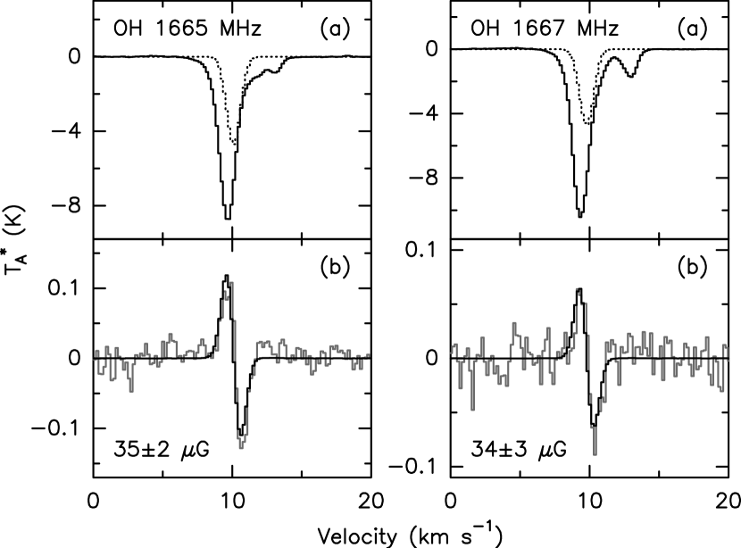
Figure New OH Zeeman measurements of magnetic field strengths in molecular clouds:

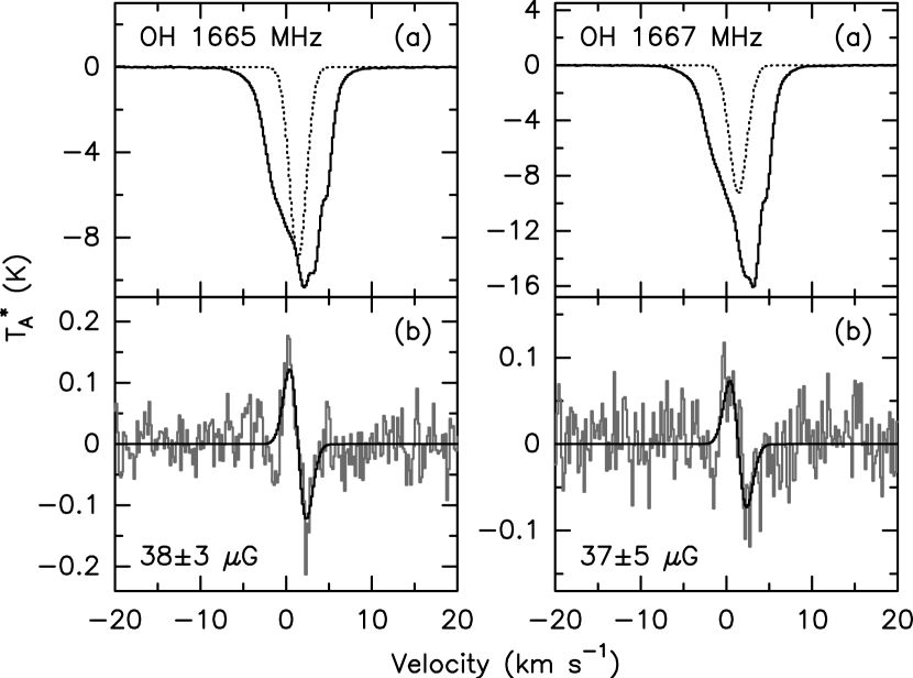
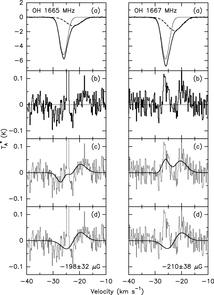
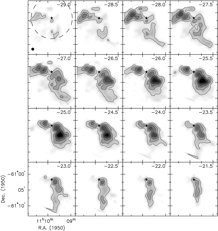
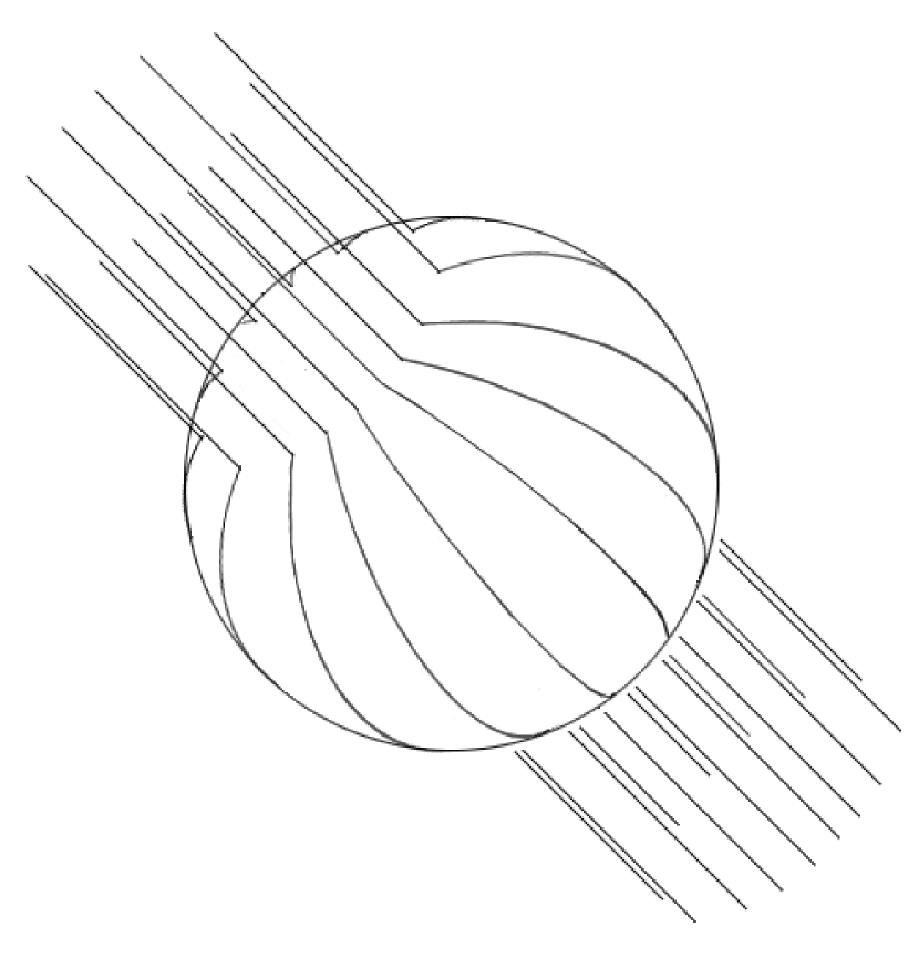
Figure New OH Zeeman measurements of magnetic field strengths in molecular clouds:

Figure New OH Zeeman measurements of magnetic field strengths in molecular clouds:

Figure New OH Zeeman measurements of magnetic field strengths in molecular clouds:

Figure New OH Zeeman measurements of magnetic field strengths in molecular clouds:

Figure New OH Zeeman measurements of magnetic field strengths in molecular clouds:

Figure New OH Zeeman measurements of magnetic field strengths in molecular clouds:

References

- (1) Allen, A., & Shu, F. H. 2000, ApJ, 536, 368
- (2) Alves, J., Petr, M., Muench, A. A., Lada, C. J., Lada, E. A., Moorwood, Cuby, J. G. 2001, in prep
- (3) Bitran, M., Alvarez, H., Bronfman, L., May, J., & Thaddeus, P. 1997, A&AS, 125, 99
- (4) Bourke, T. L., Myers, P. C., Robinson, G., & Hyland, A. R. 2001, in prep
- (5) Brand, J., van der Bij, M. D. P., de Vries, C. P., Israel, F. P., de Graauw, T., van de Stadt, H., Wouterloot, J. G. A., Leene, A., & Habing, H. J. 1984, A&A, 139, 181
- (6) Bregman, J. D., Forster, J. R., Troland, T. H., Schwartz, U. J., Goss, W. M., & Heiles, C. 1983, A&A, 118, 157
- (7) Brogan, C. L., Troland, T. H., Roberts, D. A., & Crutcher, R. M. 1999, ApJ, 515, 314
- (8) Bronfman, L., Alvarez, H., Cohen, R. S., & Thaddeus, P. 1989, ApJS, 71, 481
- (9) Brooks, K. J. 1995, Honours Thesis, Univ. Wollongong
- (10) Brooks, K. J., & Whiteoak, J. B. 2001, MNRAS, 320, 465
- (11) Brooks, K. J., Whiteoak, J. B., & Storey, J. W. V. 1998, Publ. Astron. Soc. Aust., 15, 202
- (12) Brooks, K. J., Whiteoak, J. B., & Storey, J. W. V. 2001, in prep
- (13) Cambrésy, L., Epchtein, N., Copet, E., de Batz, B., Kimeswenger, S., Le Bertre, T., Rouan, D., & Tiphène, D. 1997, A&A, 324, L5
- (14) Carpenter, J. M., Snell, R. L., Schloerb, F. P. 1990, ApJ, 362, 147
- (15) Caswell, J. L., & Haynes, R. F. 1983, Aust. J. Phys., 36, 361
- (16) Caswell, J. L., & Haynes, R. F. 1987a, Aust. J. Phys., 40, 215
- (17) Caswell, J. L., & Haynes, R. F. 1987b, A&A, 171, 261
- (18) Caswell, J. L., Haynes, R. F., & Goss, W. M. 1980, Aust. J. Phys., 33, 639
- (19) Caswell, J. L., & Robinson, B. J. 1974, Aust. J. Phys., 27, 597
- (20) Chan, S. J., Henning, Th., & Schreyer, K. 1996, A&AS, 115, 285
- (21) Crutcher, R. M. 1977, ApJ, 216, 308
- (22) Crutcher, R. M. 1979, ApJ, 234, 881
- (23) Crutcher, R. M. 1994, in ASP Conf. Ser. 65, Clouds, Cores, and Low Mass Stars, ed. D. P. Clemens & R. Barvainis (San Fransisco: ASP), 87
- (24) Crutcher, R. M. 1999, ApJ, 520, 706
- (25) Crutcher, R. M., Kazès, I. 1983, A&A, 125, L23 (CK83)
- (26) Crutcher, R. M., Kazès, I., & Troland, T. H. 1987, A&A, 181, 119
- (27) Crutcher, R. M., Roberts, D. A., Troland, T. H., & Goss, W. M. 1999a, ApJ, 515, 275
- (28) Crutcher, R. M., & Troland, T. H. 2000, ApJ, 537, L139
- (29) Crutcher, R. M., Troland, T. H., Goodman, A. A., Heiles, C., Kazès, I., & Myers, P. C. 1993, ApJ, 407, 175
- (30) Crutcher, R. M., & Troland, T. H., Lazareff, B., & Kazès, I. 1996, ApJ, 456, 217
- (31) Crutcher, R. M., & Troland, T. H., Lazareff, B., Paubert, G., & Kazès, I. 1999b, ApJ, 514, L121
- (32) Dame, T.M., Ungerechts, H., Cohen, R.S., De Geus, E.J., Grenier, I.A., May, J., Murphy, D.C., Nyman, L.-Å., & Thaddeus, P. 1987, ApJ, 322, 706
- (33) De Lara, E., Chavarría-K., C., & López Molina, G. 1991, A&A, 243, 139
- (34) Dickel, H. R., Dickel, J. R., & Wilson, W. J. 1977, ApJ, 217, 56
- (35) Dickel, H. R., Seacord, A. W., II, & Gottesman, S. T. 1977, ApJ, 218, 133
- (36) Dickel, H. R., & Wall, J. V. 1974, A&A, 31, 5
- (37) Elmegreen, B. G. 2000, ApJ, 530, 277
- (38) Frogel, J. A., & Persson, S. E. 1974, ApJ, 192, 351
- (39) Goodman, A. A. 1989, PhD. Thesis, Harvard Univ.
- (40) Goodman, A. A., Crutcher, R. M., Heiles, C., Myers, P. C., & Troland, T. H. 1989, ApJ, 338, L61
- (41) Goodman, A. A., & Heiles, C. 1994, ApJ, 424, 208
- (42) Goss, W. M. 1968, ApJS, 15, 131
- (43) Goss, W. M., Manchester, R. N., & Robinson, B. J. 1970, Aust. J. Phys., 23, 559
- (44) Hartmann, L. 2001, AJ, in press
- (45) Hayakawa, T., Mizuno, A., Onishi, T., Yonekura, Y., Hara, A., Yamaguchi, R., & Fukui, Y. 1999, PASJ, 51, 919
- (46) Heiles, C. 1988, ApJ, 324, 321
- (47) Heiles, C., Goodman, A. A., McKee, C. F., & Zweibel, E. G. 1993, in Protostars and Planets III, ed. E. H. Levy & J. I. Lunine (Tucson: Univ. Arizona Press), 279
- (48) Hildebrand, R. H., Dotson, J., L., Dowell, C. D., Platt, S. R., Schleuning, D., Davidson, J. A., & Novak, G. 1995, in ASP Conf. Ser. 73, Airborne Astronomy Symp. on the Galactic Ecosystem: From Gas to Stars to Dust, ed. M. R. Haas, J. A. Davidson, & E. F. Erikson (San Fransisco: ASP), 97
- (49) Jaffe, D. T., Stier, M. T., & Fazio, G. G. 1982, ApJ, 252, 601
- (50) Kazès, I., & Crutcher, R. M. 1986, A&A, 164, 328
- (51) Kazès, I., Troland, T. H., Crutcher, R. M., & Heiles, C. 1988, ApJ, 335, 263
- (52) Kraemer, K. E. 1998, PhD Thesis, Boston Univ.
- (53) Kraemer, K. E., & Jackson, J. M. 1999, ApJS, 124, 439
- (54) Lockman, F. J. 1989, ApJS, 71, 469
- (55) Manchester, R. N., Robinson, B. J., & Goss, W. M. 1970, Aust. J. Phys., 23, 751
- (56) Massi, F., Brand, J., & Felli, M. 1997, A&A, 320, 972
- (57) McGregor, P. J., Harrison, T. E., Hough, J. H., & Bailey, J. A. 1994, MNRAS, 267, 755
- (58) McKee, C. F. 1999, in The Origin of Stars & Planetary Systems, ed. C. J. Lada, N. D. Kylafis (Dordrecht: Kluwer), 29
- (59) McKee, C. F., Zweibel, E., Goodman, A. A., Heiles, C. 1993, in Protostars and Planets III, ed. E. H. Levy & J. I. Lunine (Tucson: Univ. Arizona Press), 327
- (60) Mac Low M.-M., Klessen R. S., Burkert, A., & Smith, M. D. 1998, Phys. Rev. Lett., 80, 2754
- (61) Mouschovias, T. Ch., & Spitzer, L. 1976, ApJ, 210, 326
- (62) Myers, P. C., Ho, P. T. P., Schneps, M. H., Chin, G., Pankonin, V., & Winnberg, A. 1978, ApJ, 220, 864
- (63) Nakano, T. 1998, ApJ, 494, 587
- (64) Nakano, T., & Nakamura, T. 1978, PASJ, 30, 671
- (65) Neckel, T. 1978, A&A, 69, 51
- (66) Padoan, P, & Nordlund, Å. 1999, ApJ, 526, 279
- (67) Persi, P., Roth, M., Tapia, M., Ferrari-Toniolo, M., & Marenzi, A. R. 1994, A&A, 282, 474
- (68) Pratap, P., Megeath, S. T., Bergin, E. A. 1999, ApJ, 517, 799
- (69) Reid, M. J., Myers, P. C., & Bieging, J. H. 1987, ApJ, 312, 830
- (70) Reid, M. J., & Silverstein, E. M. 1990, ApJ, 361, 483
- (71) Roberts, D. A., Crutcher, R. M., & Troland, T. H. 1995, ApJ, 442, 208
- (72) Roberts, D. A., Crutcher, R. M., Troland, T. H., & Goss, W. M. 1993, ApJ, 412, 675
- (73) Robinson, B. J., Goss, W. M., Manchester, R. N. 1970, Aust. J. Phys., 23, 363
- (74) Robinson, B. J., Caswell, J. L., Goss, W. M. 1971, Astrophys. Lett., 9, 5
- (75) Rodríguez, L. F., Cantó, J, Moran, J. M. 1982, ApJ, 255, 103
- (76) Sarma, A. P., Troland, T. H., Roberts, D. A., & Crutcher, R. M. 2000, ApJ, 533, 271
- (77) Sault, R. J., Killeen, N. E. B., Zmuidzinas, J., & Loushin, R. 1990, ApJS, 74, 437
- (78) Schwartz, R. D. 1991, in Loss Mass Star Formation in Southern Molecular Clouds, ESO Scientific Report 11, ed. B. Reipurth (Garching: ESO), 93
- (79) Schwartz, P. R., Thronson, H. A. Jnr., Odenwald, S. F., Glaccum, W., Loewenstein, R. F, & Wolf, G. 1985, ApJ, 292, 231
- (80) Shu, F. H., Allen, A., Shang, H., Ostriker, E. C., & Li, Z-Y. 1999, in The Origin of Stars & Planetary Systems, ed. C. J. Lada, N. D. Kylafis (Dordrecht: Kluwer), 193
- (81) Smith, C. H., Bourke, T. L., Wright, C. M., Spoon, H. W. W., Aitken, D. K., Robinson, G., Storey, J. W. V., Fujiyoshi, T., Roche, P. F., Lehmann, T. 1999, MNRAS, 303, 367
- (82) Stone, J. M., Ostriker, E. C., & Gammie, C. F. 1998, ApJ, 508, 99
- (83) Tapia, M., Roth, M., Marraco, H., & Ruiz, M. T. 1988, MNRAS, 232, 661
- (84) Tomisaka, K., Ikeuchi, S., & Nakamura, T. 1988, ApJ, 335, 239
- (85) Toriseva, M., Höglund, B., & Mattila, K. 1985, Rev. Mexicana Astron. Af., 10, 135
- (86) Troland, T. H. 1990, in Galactic and Intergalactic Magnetic Fields, ed. R. Beck, P. P. Kronberg, & R Wielebinski (Dordrecht: Kluwer), 293
- (87) Troland, T. H., Crutcher, R. M., & Kazès, I. 1986, ApJ, 304, L57
- (88) Troland, T. H., & Heiles, C. 1982, ApJ, 252, 179
- (89) Turner, B. E. 1973, ApJ, 186, 357
- (90) Turner, B. E. 1979, A&AS, 37, 1
- (91) Turner, B. E., & Heiles, C. 1971, ApJ, 170, 453
- (92) Whiteoak, J. B., & Gardner, F. F. 1974, A&A, 37, 389
- (93) Whittet, D. C. B., Prusti, T., Franco, G. A. P., Gerakines, P. A., Kilkenny, D., Larson, K. A., & Wesselius, P. R. 1997, A&A, 327, 1194
- (94) Wilking, B. A., Blackwell, J. H., Mundy, L. G., & Howe, J. E. 1989, ApJ, 345, 257
- (95) Wouterloot, J. G. A., & Brand, J. 1989, A&AS, 80, 149
- (96) Wouterloot, J. G. A., Brand, J., & Fiegle, K. 1993, A&AS, 98, 589
- (97) Wouterloot, J. G. A., & Habing, H. J. 1985, A&AS, 60, 43