Studies of multiple stellar systems – IV. The triple-lined spectroscopic system Gliese 644

Abstract

We present a radial-velocity study of the triple-lined system Gliese 644 and derive spectroscopic elements for the inner and outer orbits with periods of 2.9655 and 627 days. We also utilize old visual data, as well as modern speckle and adaptive optics observations, to derive a new astrometric solution for the outer orbit. These two orbits together allow us to derive masses for each of the three components in the system: $M_{\mathrm{A}}=0.410\pm 0.028$ (6.9%), $M_{\mathrm{Ba}}=0.336\pm 0.016$ (4.7%), and $M_{\mathrm{Bb}}=0.304\pm 0.014$ (4.7%) $M_{\odot}$. We suggest that the relative inclination of the two orbits is very small. Our individual masses and spectroscopic light ratios for the three M stars in the Gliese 644 system provide three points for the mass-luminosity relation near the bottom of the Main Sequence, where the relation is poorly determined. These three points agree well with theoretical models for solar metallicity and an age of 5 Gyr. Our radial velocities for Gliese 643 and vB 8, two common-proper-motion companions of Gliese 644, support the interpretation that all five M stars are moving together in a physically bound group. We discuss possible scenarios for the formation and evolution of this configuration, such as the formation of all five stars in a sequence of fragmentation events leading directly to the hierarchical configuration now observed, versus formation in a small N cluster with subsequent dynamical evolution into the present hierarchical configuration.

1 INTRODUCTION

This paper is the fourth in a series on triple-star systems. The overall goal of the series is to contribute to our understanding of the formation and evolution of multiple-star systems. Paper I (Mazeh, Krymolowski & Latham 1993) presented an orbital solution for the single-lined spectroscopic triple star G38-13. Paper II (Krymolowski & Mazeh 1999) developed an analytical second-order approximation for the long-term modulation of the orbital elements of triple systems. Paper III (Jha et al. 2000) analyzed the triple-lined system HD 109648, presenting observational evidence for such modulations. The present paper is devoted to the nearby triple-lined system Gliese 644.

Gliese 644 (=Wolf 630=HD 152751=HIP 82817; $\alpha$=16:55:28.76, $\delta$=$-$08:20:10.8 [J2000], $V=9.02$ mag) is a nearby system of M dwarfs at a distance of about 6 pc (Gliese 1969). The study of its multiplicity began when Kuiper (1934) discovered that Gliese 644 is a visual binary, later found to have a period of 1.7 years and semi-major axis of $0\thinspace\aas@@fstack{\prime\prime}218$ (Voûte 1946). Joy (1947) noticed large radial-velocity variations for Gliese 644, which led him to suggest that one of the two visual components is itself a spectroscopic binary with a period of a few days, making Gliese 644 one of the nearest triple systems.

Weis (1982) used photographic plates to derive a photocentric orbit and confirmed Fleischer’s (1957) suggestion that the fainter component of the visual binary, B, is more massive than the primary. He concluded that B, which is about 0.1 mag fainter than A in the visual, is the short-period spectroscopic binary. Weis derived masses of $M_{\mathrm{A}}=0.28$ and $M_{\mathrm{B}}=0.56\ {M_{\odot}}$, suggesting that the system is composed of three similar M dwarfs. These masses are consistent with the dM2.5 spectral type assigned by Henry, Kirkpatrick & Simons (1994) to the blended image of Gliese 644.

In order to learn more about Gliese 644, we started fifteen years ago to monitor the object spectroscopically. This was done within a radial-velocity study of a small sample of nearby M dwarfs carried out with the facilities at the Harvard-Smithsonian Center for Astrophysics (CfA). From the beginning of the project we could see two and occasionally even three peaks in some of the one-dimensional cross-correlation functions, which were obtained by correlating the spectra of Gliese 644 against our standard observed M-star template. Given the visual orbit of the outer binary, the triple-lined nature of Gliese 644 makes this system special, as it enables us to derive individual masses for each of the three components if spectroscopic solutions can be derived for both the inner and the outer orbits. This can add important information about the mass-luminosity relation in the solar vicinity (cf. Andersen 1991, Söderhjelm 1999) near the bottom of the Main Sequence (e.g., Henry et al. 1999).

The derivation of radial velocities for all three components in the Gliese 644 system presented an unusually difficult challenge, because the inner and outer orbits both have small radial-velocity amplitudes, resulting from the nearly face-on inclination of the outer orbit, $i\sim 165\degr$, from the relatively long period of the outer orbit, $P\sim 1.7$ yr, and from the relatively small masses of the three stars, $M\sim 0.3$ $M_{\odot}$. The lines from all three stars are rarely resolved in our spectra; in most cases all three are blended together. To solve the problem of extracting velocities for all three stars from blended spectra, we had to wait for the development of a more powerful algorithm than the one-dimensional cross-correlation techniques that we had been using. Such an algorithm is TODCOR (Zucker & Mazeh 1994), which was developed originally as a two-dimensional correlation technique for extracting velocities for both stars in double-lined spectroscopic binaries, even when the two sets of lines were not resolved. The extension of TODCOR to three dimensions for the analysis of triple-lined systems (Zucker, Torres & Mazeh 1995) provided us with the tool that we needed to analyze the spectra of Gliese 644.

Even with TODCOR, the extraction of radial velocities for all three components of Gliese 644 proved to be difficult. To address this difficulty, we developed a new approach for solving spectroscopic orbits for systems with composite spectra. The new approach searches a model that includes the observed spectra together with the orbital parameters of the system. The final model is the one that gives the best match between the observed spectra and the corresponding set of composite spectra predicted by the model.

The observations were analyzed with this approach by two different teams, one at Tel Aviv and the other at the CfA, with some differences in the details at various stages of the analysis. The two analyses led to similar results, and most of the orbital elements agreed within the internal uncertainty estimates. However, the velocity amplitudes for the outer orbit disagreed by 3.2 and 3.5 times the internal error estimates, suggesting the presence of significant systematic difference between the two analyses. Therefore, we present the results from both analyses and document the procedures used in detail. For the final orbital parameters we adopt simply the averages of the values derived by the two analyses.

Visual observations of the wide pair Gliese 644AB extend back more than 50 years. Because some recent unpublished speckle observations were available to us, we decided to reanalyze the astrometric orbit of the outer binary. Comparison between the results of the spectroscopic and astrometric analyses indicates some possible systematic scale differences between the two sets of data. This impression was supported by the observations and analysis of Gliese 644 by Ségransan et al. (2001), a work published about three months after we submitted our paper, while our paper was still being reviewed. Their astrometric orbit, which was based solely on speckle and newly obtained adaptive optics (AO) measurements and did not include any visual observations, yielded a somewhat larger semi-major axis. We find a similar trend when we use only the modern astrometric observations to estimate the semi-major axis. Because of the importance of the scale of the astrometric orbit for the mass determinations, and because the visual observations are more likely to be afflicted by systematic errors, we decided to rely only on the modern data to set the scale of the orbit.

The details of the visual analysis are reported in section 2. A new approach for solving spectroscopic orbits of systems with composite spectra is described in Section 3, together with the details of the Tel Aviv and CfA orbital solutions. In Section 4 the solutions for the spectroscopic and astrometric orbits are combined to solve for the individual masses of the three M stars in the Gliese 644 system. Section 5 discusses in detail the visual and IR photometry we have in hand for the A and B components of the system, and Section 6 considers the impact of our results on the mass-luminosity relation near the bottom of the Main Sequence. Section 7 discusses the relationship of Gliese 644 to Gliese 643 and vB 8, two nearby common-proper-motion companions. Our radial-velocity measurements support the interpretation that all five stars are moving together in a physically bound system. In the final section we summarize our results and discuss the implications for two scenarios describing the formation and evolution of binary and multiple systems.

2 THE ASTROMETRIC ORBIT FOR THE OUTER BINARY

2.1 The visual and speckle data

For nearly 50 years Gliese 644AB was the shortest-period (1.7 yr) binary resolved by visual means, with an angular separation of $\sim$0 $\aas@@fstack{\prime\prime}$2. Only when interferometric and speckle techniques became available was it possible to resolve systems with even smaller separations. Consequently, Gliese 644AB attracted a great deal of attention, and a large number of visual observations have accumulated since its discovery.

The history of the astrometric observations of Gliese 644AB is far from uniform. During the first five seasons after its discovery more than 270 visual measurements were made, approximately 200 of them by the same observer, J. G. Voûte, at the Bosscha Observatory in Lembang, Java. Voûte was also the first to publish an orbit for the system (Voûte 1946). In the following 45 years some 80 additional visual observations were collected by a number of observers. The cumulative distribution of all the visual observations is shown in Figure 1, where the irregular pattern is obvious.

Figure 1: Cumulative distribution of the visual observations.

In recent years speckle observations of Gliese 644AB have also been made at both visual and infrared wavelengths, providing additional measurements of both the separation and the relative brightness of the two wide components. Three of the speckle measurements were obtained by one of us (Henry 1991) in the infrared ($J$, $H$, $K$), using the Steward Observatory 2.3-m telescope on Kitt Peak, and have not appeared in the literature. Two are one-dimensional scanning observations in the North-South direction, and one is a two-dimensional observation. Descriptions of the instrumentation and observing techniques can be found in McCarthy (1986) for the one-dimensional speckle observations, and McCarthy et al. (1991) for the two-dimensional speckle observation. Finally, Ségransan et al. (2001) have very recently reported five adaptive optics measurements that are of very high precision.

A listing of all the astrometric observations, with the exception of the three speckle measurements mentioned above and the AO measurements, was provided to us by the late Charles E. Worley (U.S. Naval Observatory) and was extracted from the Washington Double Star Catalog (Worley & Douglass 1996). The three unpublished speckle observations are listed in Table 1. The type of measurement is indicated by “2ds” (two-dimensional speckle) or “1ds” (one-dimensional speckle).

Table 1: Unpublished speckle observations for Gliese 644AB.

Date	Orbital	$\theta$	$\rho$
(Year)	Phase	(deg)	(arcsec)	Type
1984.3570	0.797		0.13	1ds
1989.2220	0.631		0.17	1ds
1990.3530	0.289	301	00.198	2ds

With this wealth of information covering nearly 40 orbital cycles (1934-2000) it should in principle be straightforward to obtain a high-quality solution for the visual orbit. Indeed, a number of solutions have been published since Voûte’s first determination (e.g., Starikova 1980, Heintz 1984), although the original orbit is the one listed as “definitive” in the Fourth Catalog of Orbits of Visual Binary Stars (Worley & Heintz 1984). The combination of the old and the new data can in principle improve the orbital solution. This prompted us to take the present study of Gliese 644 as an opportunity to rediscuss the visual orbit.

2.2 The orbital solution

Using all the available astrometric observations together raises two problematic issues. The first has to do with the variety of observers, observing conditions, and techniques used to collect the astrometric data since 1934, which could give rise to systematic errors. The second and more fundamental issue is associated with the triple nature of Gliese 644, which introduces tidal interactions between the outer and inner orbits. This could produce slow changes in the elements of the outer orbit (as well as the inner orbit) on long timescales (e.g. Mazeh & Shaham 1976, 1977). The timescale for a complete cycle of such a modulation is of the order of 700 years (Mazeh & Shaham 1979), while the actual timescale could be shorter. Thus we cannot rule out a priori some small changes in the elements of the wide orbit during the 66 years of observational coverage.

In order to address the first of these issues, we begin by pointing out a potentially serious shortcoming of the observations obtained by the visual technique. These data are dominated in number by the measurements made by Voûte, who observed with a 60-cm refractor. At visual wavelengths the diffraction limit of such an instrument is approximately 0$\aas@@fstack{\prime\prime}$23, which is essentially the same as the angular separation displayed by Gliese 644AB throughout its entire orbit. In his original publications Voûte reports that the measurements are frequently only “estimates” made from elongated or notched images. Under these conditions angular separation measurements by the visual technique must be taken with extreme caution, since they have often been shown to be biased (see, e.g., Douglass & Worley 1992) and could affect the semimajor axis of the orbit. Nevertheless, the visual observations are potentially valuable for the extended time coverage they provide. Consequently, we started by considering a solution that incorporates only the visual measurements and none of the modern speckle or AO observations, which could have a different scale. Evidence of just this effect is discussed below.

To compute the orbital solutions described in this section we used standard non-linear least-squares techniques based on the Levenberg-Marquardt method (Press et al. 1992). All position angles were precessed to the epoch 2000. The solutions were obtained iteratively, solving for an orbit and adopting the root mean square residual as the uncertainty for the next iteration, until convergence. The errors determined through this procedure are 0 $\aas@@fstack{\prime\prime}$012 and 0 $\aas@@fstack{\prime\prime}$013/$\rho$, which are surprisingly good for the visual technique. Eight observations gave unusually large residuals in these preliminary solutions ($\gg 3\sigma$), and were rejected. Observations in which only the angular separation was discrepant were not entirely rejected, because the position angles can still be accurate (they are measured essentially independently from the separations in both the visual and the speckle techniques). These observations can contain valuable information on the period of the system, and should be included in the solution.

The residuals from a solution using only the visual data are shown in Figure 2. Unusual trends are seen in the residuals of both $\theta$ and $\rho$, plotted here as a function of position angle in the orbit. The bottom panel shows an obvious pattern of parallel curves separated by exactly 0 $\aas@@fstack{\prime\prime}$01, which is the precision to which visual observers typically read off the separations from their filar micrometers. A less obvious effect is seen in the $\theta$ residuals displayed in the top panel, which seem to change sign on either side of 90° and 270° (shown as vertical dotted lines). In addition, when plotted as a function of time (not shown here), the residuals in $\theta$ are systematically negative by about 5° during 1935, which was the first of Voûte’s very intensive observing seasons for Gliese 644.

Figure 2: Residuals in $\theta$ and $\rho$ from an astrometric orbit that uses only visual data, shown as a function of position angle.

To further investigate the latter effect we performed a sequence of additional orbital solutions in which we removed the older measurements one by one and recomputed the orbital elements in each case. These fits are therefore not independent, and perhaps a better way would be to compute solutions in a window corresponding to a fixed interval of time or a fixed number of observations, sliding it along the time axis. Unfortunately the peculiar time history for the astrometry of Gliese 644, with more than 75% of the data obtained in the initial 10% of the time coverage, does not allow this (see Figure 1). As a result of this exercise, we detected sharp changes in the orbital elements as soon as the observations in 1935 are excluded. Although tidal effects as discussed earlier can produce long-term changes in the orbital elements, the discontinuities observed are much to abrupt to be real. An alternate explanation would be a systematic error in the observations for 1935, the vast majority of which were made by Voûte. From the discussion above it appears likely that his position angles include a systematic error. This is somewhat unexpected for such a careful and experienced observer as Voûte, particularly since his later observations do not show this effect. There are no clues on the source of the systematic error, despite the fact that he recorded his observations in great detail, and we can only speculate as to the cause. We have therefore chosen to exclude Voûte’s first observing season altogether, after which the discontinuities in the orbital elements mentioned above disappear completely.

The remaining visual observations, which cover nearly 50 years, were used to examine the possibility of changes in the orbital elements due to tidal effects. For this we divided the measurements into two independent groups, although once again as seen in Figure 1 the time sampling is not very favorable for this sort of test. As a compromise between the number of orbital cycles spanned and the number of observations in each group, we chose 1955 as the dividing point. Independent solutions using the pre-1955 and post-1955 data are given in Table 2.

Table 2: Astrometric orbital solutions for Gliese 644AB, excluding the 1935 observations by Voûte.

Element	Pre-1955	Post-1955	All visual	Modern	Adopted
	(visual only)	(visual only)		(no visual)
$P$ (yr)	$1.71576\pm 0.00058$	$1.71634\pm 0.00088$	$1.71687\pm 0.00018$	$1.71671\pm 0.00091$	$1.717267\pm 0.000039$
$P$ (d)	$626.67\pm 0.21$	$626.89\pm 0.32$	$627.087\pm 0.066$	$627.03\pm 0.33$	$627.232\pm 0.014$
$a(\arcsec)$	$0.2169\pm 0.0013$	$0.2143\pm 0.0035$	$0.2166\pm 0.0013$	$0.2238\pm 0.0023$	$0.2256\pm 0.0011$
$e$	$0.0337\pm 0.0026$	$0.0666\pm 0.0082$	$0.0384\pm 0.0026$	$0.0448\pm 0.0066$	$0.0433\pm 0.0018$
$i(\degr)$	$165.0\pm 1.7$	$163.2\pm 5.1$	$164.9\pm 1.6$	$166.9\pm 6.1$	$163.1\pm 1.6$
$\omega(\degr)$	$124.4\pm 7.7$	$83\pm 17$	$118.9\pm 7.2$	$98\pm 40$	$115.6\pm 5.1$
$\Omega_{2000}(\degr)$	$169.7\pm 6.4$	$140\pm 17$	$167.2\pm 6.3$	$150\pm 26$	$163.2\pm 3.1$
$T$	$1988.111\pm 0.024$	$1988.083\pm 0.036$	$1988.129\pm 0.017$	$1988.122\pm 0.067$	$1988.143\pm 0.011$
$a^{3}/P^{2}({\mathrm{arcsec}}^{3}{\mathrm{yr}}^{-2})$	$0.003468\pm 0.000058$	$0.00334\pm 0.00021$	$0.003446\pm 0.000063$	$0.00380\pm 0.00020$	$0.003893\pm 0.000058$
$N_{\theta}$	231	39	270	14	284
$N_{\rho}$	219	37	258	13	13
$N_{\mathrm{1}-D}$	0	0	0	1	1
Span (yr)	19.1	26.0	48.9	16.0	66.0

The orbital elements derived from the two data sets are rather similar, with the exception of the eccentricity. The change in $e$ amounts to 3.8 times the combined errors, an apparently significant effect. Interestingly enough, this is one of the parameters expected to vary due to the tidal interaction between the outer and inner orbits, and for some triples it displays the most prominent modulation (Mazeh & Shaham 1979; Paper II). Although very suggestive, we hesitate to place much confidence in this result at the present time in view of the systematic trends in the visual data illustrated in Figure 2, which could alter the shape of the orbit in subtle ways. Nevertheless, continued observations with modern techniques may well confirm this in the future. A combined solution using all the visual data together is shown in the third column of the table.

Because of the potential for systematic errors in the angular separations of the visual data, a completely independent solution was carried out using only the modern speckle and AO measurements. The one-dimensional speckle observations also contain useful information on the angular separation, and can be included in the fit as well. We assigned errors for the (two-dimensional) speckle measurements of 0 $\aas@@fstack{\prime\prime}$01 in angular separation ($\rho$) and 0 $\aas@@fstack{\prime\prime}$01/$\rho$ in position angle ($\theta$). For the one-dimensional speckle measurements we adopted an error of 10 percent. We note, however, that the uncertainties reported by Ségransan et al. (2001) for their five AO measurements are substantially smaller than those of the speckle measurements, with the result that they carry a very large weight in this new fit. Two of those observations, in particular, have quoted errors in the angular separation of only 0$\aas@@fstack{\prime\prime}$0005. If allowed to carry this enormous weight (400 times that of the speckle technique), these AO measurements would completely dominate the solution, a risky situation when little is known about the systematic errors they may be affected by. We have preferred to be conservative, and have therefore chosen to set the errors in angular separation of these two AO observations to the average of the other three, which is 0$\aas@@fstack{\prime\prime}$003.

The new fit based exclusively on modern observations is shown in the fourth column of Table 2. Compared to the solution that uses all the visual data, uncertainties in all the elements are larger due to the smaller number of observations and the shorter time coverage. Still, the elements of the two fits are consistent within 1$\sigma$, with the exception of the semimajor axis (2.7$\sigma$), which is larger in the modern fit than indicated by the visual solution.

Similar indications come from a semi-independent solution published for the astrometric orbit based on data from the Hipparcos mission. Gliese 644AB was one of the targets observed by the satellite (HIP 82917), and although the orbital elements are not actually listed in the Hipparcos Catalogue (ESA 1997), a re-analysis of the intermediate transit data was performed by Söderhjelm (1999) as part of a study of 205 binary systems. Ground-based observations were incorporated to some extent in Söderhjelm’s analysis, so that his solution for Gliese 644AB is not completely independent of ours. Nevertheless, the semimajor axis he obtained, $a=0\aas@@fstack{\prime\prime}23$, is larger than suggested by the visual data, possibly due to his reliance on the very precise satellite measurements to set the scale.

As mentioned earlier, many of the angular separations measured visually are merely estimates that were made at or under the resolution limit of the telescope, and as such they are particularly susceptible to personal (i.e., subjective) errors. It seems safer, therefore, to rely on the modern speckle and adaptive optics measurements to set the scale, since these are considerably more objective in nature. On the other hand, the position angles of the visual measurements may still be useful since they are typically more accurate than the angular separations (see, e.g., Pannunzio et al. 1986). The optimal solution for Gliese 644AB, therefore, is one that uses the modern data (both $\theta$ and $\rho$) mainly for scale, and the visual position angles that provide the time coverage to strengthen the orbital period. Subtle effects such as those illustrated in the top panel of Figure 2 will tend to cancel out over many cycles and will not otherwise affect the solution significantly because of the much smaller weight of the visual data. The result of this combined fit is given in the last column of Table 2, and these are the orbital elements we adopt for the remainder of this paper.

Figure 3: The astrometric orbit and the observations on the plane of the sky. The scale is set solely by speckle and AO measurements (see text). The plus signs represent the visual observations, and the triangles and circles are for the speckle and AO measurements, respectively. Motion is clockwise.

A graphical representation of the orbit and the observations on the plane of the sky are shown in Figure 3. As expected, the visual observations fall mostly inside the orbit, since the angular separations are typically underestimated, as discussed above.

Our new orbital solution is in good agreement with the old astrometric solutions, except for the scale. The plane of the orbit is highly inclined (only $15\degr$ from face on), the motion is retrograde, and the orbit is nearly circular, with a very small but significant eccentricity. When only an astrometric orbit is available, the values of $\omega$, the longitude of the periastron, and $\Omega$, the position angle of the ascending node, are both ambiguous by $180\degr$. The values quoted in Table 2 eliminate this ambiguity by taking into account the spectroscopic orbit presented below. In particular, the relative motion of the secondary is away from the Sun at the ascending node.

The inclination angle we derive, $i=163\aas@@fstack{\circ}1\pm 1\aas@@fstack{\circ}6$, is slightly larger than the values by Ségransan et al. (2001) ($i=160\aas@@fstack{\circ}3\pm 0\aas@@fstack{\circ}1$) and Söderhjelm (1999) ($i=161\degr$), although in the latter case no errors are given and it is difficult to evaluate the results. On the other hand, the eccentricity found by Söderhjelm (1999), which presumably corresponds on average to a fairly recent epoch because of the use of the Hipparcos measurements, is $e=0.06$, which is very close to the value we obtain from the post-1955 visual data. This would seem to support the difference we noted earlier, but until stronger evidence is found all we can say at the moment is that the ground-based and Hipparcos data cannot rule out a possible slight increase in the eccentricity of the outer orbit of Gliese 644 on a long timescale.

3 THE SPECTROSCOPIC ORBITS FOR THE INNER AND OUTER BINARIES

We have monitored the spectrum of Gliese 644 with the CfA Digital Speedometers (Latham 1985, 1992), using three nearly identical instruments. Most of the spectra were obtained with the 1.5-m Tillinghast Reflector at the F. L. Whipple Observatory atop Mt. Hopkins, Arizona (113 exposures) and the 1.5-m Wyeth Reflector located at the Oak Ridge Observatory in the town of Harvard, Massachusetts (77 exposures). A few of the spectra were obtained with the MMT, also located at the Whipple Observatory (10 exposures). Photon-counting intensified Reticon detector systems were used to record a single echelle order centered near 5187 Å, with a spectral coverage of 45 Å and resolution of 8.3 km s^-1. The signal-to-noise ratio ranged from 7 to 40 per resolution element in the continuum, with 20 being a typical value. The first 194 exposures were obtained over a 2645-day span between 1984 and 1991, while the final 6 exposures were obtained 10 years later in 1997.

To analyze the data we developed a new approach in which a candidate model for the system and its two spectroscopic orbits is judged by how well it reproduces the set of observed spectra. For the sake of simplicity we choose to discuss our approach only for the case of a double-lined binary. Extending our approach to the triple-lined case is straightforward.

3.1 The New Approach

3.1.1 The old procedure

In previous studies of double-lined systems (e.g., Mazeh et al. 1995, Goldberg et al. 2000) we have derived orbital solutions in two separate steps. In the first step we extracted individual radial velocities for the two stars from each of the observed spectra. Then in the second step we derived the orbital parameters, based on the velocities obtained in the first step. The velocity extraction was accomplished using TODCOR, a two-dimensional correlation technique (Zucker & Mazeh 1994) that assumes the observed spectrum is a combination of two spectra, with shifts caused by the radial velocities of the two components. The algorithm calculates the correlation of the observed spectrum against a combination of two templates with different shifts. The result is a two-dimensional correlation function, whose maximum is expected at the shifts corresponding to the actual velocities of the two components. To find the orbital solutions of the binary systems we used ORB (Paper I) — a code that searches the orbital parameter space for a minimum of the residuals of the stellar radial velocities.

To derive the radial velocities of the two stars TODCOR requires two template spectra, one for the primary and the other for the secondary. To match the actual components of each binary we chose templates from a library of synthetic or observed spectra. To optimize the match between the templates and the observed composite spectra, we ran TODCOR for a variety of different templates from the library. To each pair of templates we assigned a measure of its fit to the spectra of the binary – the peak correlation obtained by TODCOR for that pair of templates, averaged over all the observed spectra. We then chose the pair of templates that gave the highest average value for the peak.

To extract the radial velocities for the two stars, the brightness ratio of the two templates, $\alpha$, is also needed. For each observed spectrum TODCOR can derive the radial velocity of the two components either by accepting a predetermined brightness ratio or by finding the best ratio to fit that spectrum at the velocities found. Normally we assumed the binary system had the same brightness ratio for all the observed spectra, and therefore adopted a single value of $\alpha$ for all the spectra. To choose the best brightness ratio we either averaged the derived $\alpha$ values over the observed spectra, or ran TODCOR for a grid of predetermined $\alpha$ values, searching for the value that gave the highest average value for the peak.

Choosing the best templates and best value for $\alpha$ comprised the major part of the first step of the old procedure. Only after the templates and the brightness ratio had been established did we proceed to derive the radial velocities, which were then used by ORB to find the orbital solution.

3.1.2 A modified approach

The separation of the reduction procedure into the two steps described above is somewhat artificial and is not necessarily the optimum way to find the best model for the system. We describe here a new approach, based on the philosophy that the model as a whole, namely the orbital elements together with the choice of templates and brightness ratio, should be confronted directly with the observed spectra. In short, we propose that for any suggested model of the system one should construct a set of predicted spectra and compare them with the observed spectra.

This confrontation can be done in a straightforward way. Consider a model consisting of a given set of values for the orbital parameters together with a choice of templates and brightness ratio. First, derive two stellar velocities predicted by the orbital parameters for the timing of each of the observations. Second, construct a predicted spectrum for each observation by shifting the templates with the predicted velocities and combining the two shifted templates with the adopted brightness ratio. To compare the predicted spectrum with the observed one, calculate the correlation between the two spectra. Finally, the correlations of the different observed spectra should be combined into a global score, which measures the match of all the spectra to the model.

Note that in this new approach the correlation calculated for an individual observed spectrum is the correlation at the velocities predicted by the orbital solution. This is not necessarily the highest possible correlation for that observed spectrum. There might be a different pair of velocity shifts for the two templates that yields a higher correlation. However, in the new approach what counts is the correlation corresponding to the two velocities predicted by the specific orbital solution, calculated for the time of the observation.

The best model is the one that yields the highest correlation score. Therefore, the algorithm we propose performs a search for the best model in the complete parameter space, which includes the orbital parameters and the possible templates and brightness ratios. To perform an efficient search we suggest an iterative procedure. The solution found in the old approach serves as our first guess. This gives us a choice of templates and brightness ratio, together with an orbital solution. We then iterate, so that every stage of the iteration consists of three steps:

• A search for the best templates and brightness ratio, given the velocities predicted by the previous orbital solution.

• A new TODCOR derivation of stellar velocities, given the new templates and brightness ratio.

• The determination of a new orbital solution with ORB, by minimizing the $\chi^{2}$ of the residuals with regard to the new velocities.

We require that each step yields a higher correlation score, and that the iterations converge.

The extension of the new approach to triple-lined systems is straightforward. We need to search for three templates and two brightness ratios, $\alpha$ and $\beta$, one corresponding to the ratio between the secondary and the primary brightness, the other to the ratio between the tertiary and the primary.

3.2 Analysis

The lines of the three stars of Gliese 644 are blended in most of our observed spectra. It is therefore especially important to have good template spectra, optimized to match each of the three components. In particular, it is important that the template spectra have the correct rotational broadening when using TODCOR to determine radial velocities from blended spectra. If there is not enough rotational broadening in the templates, TODCOR is forced to pick orbital velocities that are too far apart, in order to match the observed line broadening. Conversely, TODCOR will pick orbital velocities that are too close if the templates have too much rotational broadening.

For most of our radial-velocity projects we use template spectra drawn from an extensive library of synthetic spectra calculated by Jon Morse for a large grid of Kurucz model atmospheres (cf. Nordström et al. 1994, Morse & Kurucz in preparation). Synthetic templates have the advantage that they can be calculated for dense grids in effective temperature, surface gravity, metallicity, and rotational broadening. If observed spectra are used as templates, it is hard to find real stars that fill densely such grids. Unfortunately, the Kurucz models start to become increasingly unrealistic for effective temperatures below about 4000 K. For M dwarfs we have found that we get better correlations if we use templates drawn from a small library of observed spectra with spectral types in the range K7 to M5.5. The observed templates available for our analysis of Gliese 644 are summarized in Table 3, where we list the stellar spectral types of Henry et al. (1994).

Table 3: The stars observed for templates.

Gliese	$\alpha$  (J2000)  $\delta$	$V$	Spectral
		(mag)	Type
380	10:11:22.14  +49:27:15.3	6.61	K7
809	20:53:19.79  +62:09:15.8	8.54	M0.0
846	22:02:10.27  +01:24:00.8	9.16	M0.5
908	23:49:12.53  +02:24:04.4	8.98	M1.0
15A	00:18:22.89  +44:01:22.6	8.07	M1.5
49	01:02:38.87  +62:20:42.2	9.56	M2.0
745B	19:07:13.22  +20:52:36.2	10.75	M2.0
48	01:02:32.23  +71:40:47.3	9.96	M2.5
725A	18:42:46.66  +59:37:50.0	8.91	M3.0
725B	18:42:46.90  +59:37:36.6	9.69	M3.5
273	07:27:24.50  +05:13:32.8	9.89	M3.5
699	17:57:48.50  +04:41:36.2	9.54	M4.0
51	01:03:12.22  +62:21:54.2	13.66	M5.0
905	23:41:54.02  +44:09:32.	12.28	M5.5

Throughout our iterations two sets of templates performed significantly better than any others we tried: Gliese 725A for the primary and Gliese 725B for the secondary and tertiary, and Gliese 725A for the primary and Gliese 273 for the secondary and tertiary. These sets gave essentially the same peak correlation averages. We decided to adopt the Gliese 725 templates, because we hoped that this would minimize systematic errors due to differences in velocity zero points, metallicity, and rotational velocity.

To find the brightness ratio and the orbital parameters we have developed two independent procedures, one at Tel Aviv and the other at the CfA. Completely independent codes were used throughout, both for the implementation of TODCOR and for the orbital solutions. We describe the two procedures in the next two subsections.

3.2.1 The Tel Aviv Analysis

To find the brightness ratios of Gliese 644 we ran in each iteration a grid of $\alpha$ and $\beta$, using all 200 velocities derived in the previous iteration. To average the different correlations calculated for the different observed spectra we used a “generalized correlation score” derived by Zucker (in preparation) by applying a maximum-likelihood approach. This score can be thought of as a way of weighting the individual correlations by using the estimated signal-to-noise ratio of each spectrum. We finally converged to a value of $\alpha=0.56\pm 0.06$ and $\beta=0.36\pm 0.04$.

Finding the orbital solutions of a triple-lined system for a given set of velocities is somewhat more complicated than in the case of a double-lined binary. This is so because we have to solve for two orbits, one for the close pair and the other for the center of mass of the close pair together with the distant third star. To solve simultaneously for the two orbits we use the code ORB.20, a slightly modified version of ORB.18 (Paper I). The solution is reached in a few iterative steps. First, ORB solves for the orbital elements of the primary, whose sole motion is within the wide orbit. Second, ORB solves for the orbital elements of the primary and the secondary as a double-lined system in the wide orbit, ignoring at this stage the short-period motion of the secondary. Third, it solves for the elements of the primary and the secondary as a triple system, taking into account for the first time the secondary short-period motion. At this stage the wide orbit is considered as a double-lined orbit, while the short-period orbit is considered as a single-lined one. Then, in the last stage of the solution, the tertiary data are taken into account, and the short-period motion is considered as a double-lined orbit. Each step of the iteration is used as the starting point for the next one. Finally, we compute differential corrections for all the elements of the two orbits together.

It has been our experience that the period is the critical parameter of the orbital solution, so ORB first searches the orbital parameter space with a dense grid of fixed values of the orbital period, covering a range of periods given by the user. For every value of the period ORB searches for the parameters that minimize $\chi^{2}$. This procedure ensures that we do not miss any local minimum in the parameter space of the orbital elements. Only when the best period has been found, does ORB execute an iterative algorithm to find the best set of parameters to fit the data.

The velocities derived with TODCOR can encounter two problems, both resulting from the fact that all observed spectra include some noise. The problems have to do with the fact that TODCOR derives the three velocities from the location of the highest peak of the correlation in the three-dimensional velocity space. One problem occurs when a spurious peak of the three-dimensional correlation gets randomly enhanced by the noise and becomes higher than the peak that corresponds to the actual three velocities. In such a case TODCOR can chose a completely wrong peak. Another problem occurs when TODCOR switches between the velocities of the three stars. This can happen when the templates are similar and the spectra have poor signal-to-noise ratios. Both problems can generate outlier velocities with large residuals.

To minimize the problem of identifying a completely wrong peak we let TODCOR search for a peak in a limited region of the three dimensional space, centered on the point which corresponds to the three velocities predicted by the orbital solution from the previous iteration. Usually a range of $\pm 35$ km s^-1 in each dimension is searched. To identify velocities switched by TODCOR we search for exposures where the three derived velocities yield a high $\chi^{2}$ when compared to the velocities predicted by the orbital solution. We then switch the velocities if and only if the switched velocities give a significantly smaller $\chi^{2}$ for that exposure. After switching velocities we then iterate the entire orbital solution again and require that the new solution give a lower $\chi^{2}$.

The individual radial velocities and (O-C) residuals from the orbital solutions are reported in Table 4.

Table 4: Radial velocities and residuals (km s^-1) for Gliese 644 (first 20 lines)

IIIIHJD	Gliese 644A				Gliese 644Ba				Gliese 644Bb
(2,400,000$+$)	CfA		Tel Aviv		CfA		Tel Aviv		CfA		Tel Aviv
	$V_{\rm{r}}$	(O $-$ C)	$V_{\rm{r}}$	(O $-$ C)	$V_{\rm{r}}$	(O $-$ C)	$V_{\rm{r}}$	(O $-$ C)	$V_{\rm{r}}$	(O $-$ C)	$V_{\rm{r}}$	(O $-$ C)
45817.8613	10.88	$-$0.42	11.84	$+$0.80	30.70	$+$8.90	30.22	$-$0.32	11.52	$-$0.68	6.00	$+$2.94
46461.9627	14.50	$-$1.12	11.81	$+$0.21	10.80	$+$4.02	16.38	$+$4.50	27.24	$+$2.46	26.34	$+$3.50
46464.9225	11.00	$+$3.89	14.55	$+$2.84	15.95	$+$2.93	9.33	$-$2.71	25.86	$-$1.14	24.62	$+$2.11
46485.9236	12.21	$-$1.47	12.13	$-$0.40	2.44	$-$0.15	2.91	$-$0.93	30.81	$-$0.69	29.15	$-$1.25
46487.9269	13.30	$-$0.21	13.01	$+$0.39	32.38	$-$1.36	32.42	$+$0.66	$-$2.20	$+$0.32	1.08	$+$1.59
46489.9227	13.79	$-$1.94	11.69	$-$1.01	13.02	$+$3.03	16.63	$+$1.66	21.57	$+$0.73	18.04	$+$0.16
46492.9182	12.72	$+$0.18	11.60	$-$1.24	16.14	$+$1.22	13.09	$-$2.83	18.49	$-$0.47	16.24	$-$0.40
46511.9706	14.13	$+$0.45	13.66	$-$0.06	25.44	$-$1.26	23.49	$-$0.87	4.91	$+$0.07	5.38	$-$0.71
46512.8394	14.77	$+$1.37	13.92	$+$0.16	0.42	$+$0.02	$-$0.22	$+$0.88	34.80	$+$0.67	31.27	$-$2.85
46513.8548	14.82	$-$0.15	14.01	$+$0.20	21.46	$-$1.52	21.59	$+$0.25	8.26	$+$0.67	7.63	$-$1.66
46520.0076	14.34	$-$0.71	14.01	$-$0.10	27.21	$-$1.20	25.54	$-$1.79	1.23	$-$0.12	2.75	$+$0.49
46520.8817	15.08	$+$0.03	14.93	$+$0.78	24.31	$-$0.47	23.74	$+$0.10	5.93	$+$0.58	6.23	$-$0.04
46523.8260	14.33	$+$0.45	13.75	$-$0.54	25.28	$-$4.27	22.28	$-$1.90	1.32	$-$0.32	4.19	$-$1.29
46537.9235	15.75	$+$0.79	15.43	$+$0.43	30.70	$+$0.90	28.82	$-$0.29	$-$0.04	$+$0.38	0.46	$+$1.42
46538.9682	12.11	$+$5.30	12.37	$-$2.68	18.73	$+$3.45	18.90	$+$5.80	20.65	$-$3.31	17.43	$+$0.80
46539.8366	15.35	$-$0.43	15.50	$+$0.41	$-$1.29	$-$0.54	$-$1.39	$-$0.38	32.39	$-$0.12	31.86	$-$0.28
46540.8298	15.00	$-$0.40	15.75	$+$0.61	28.30	$-$0.80	27.17	$-$0.81	$-$0.60	$-$0.52	1.34	$+$1.24
46540.9278	15.31	$-$0.24	15.22	$+$0.07	30.19	$-$0.65	29.13	$-$0.46	$-$2.37	$-$0.21	$-$3.06	$-$1.36
46541.8861	14.86	$+$1.45	14.03	$-$1.17	16.54	$-$3.58	13.08	$-$1.63	11.59	$-$0.71	17.12	$+$2.48
46565.7149	16.63	$+$1.18	15.66	$-$0.72	11.68	$+$1.31	11.81	$+$1.66	20.00	$-$0.15	20.92	$+$2.91

The elements for the spectroscopic orbits derived by the Tel Aviv team are given in Table 5. For four of the observed spectra the assignment of the three velocities to the three stars in the system was swapped from the initial assignment made by TODCOR in order to improve the overall $\chi^{2}$ of the solution, as described above. We denote the orbit of Ba and Bb by B, and the orbit of A and B by AB. The period, eccentricity, longitude of periastron, and the time of periastron passage are denoted by $P,e,\omega$ and $T$, respectively. The radial-velocity semi-amplitudes of A and B are denoted by $K_{\mathrm{A}}$ and $K_{\mathrm{B}}$. Similar notations are used for Ba and Bb. We also report the light ratios derived using TODCOR in Table 5. The errors in the light ratios were estimated using an analysis of the $\chi^{2}$ values near the peak of the three-dimensional correlation surface. These errors should include the effects of photon noise, but do not take into account possible systematic errors due to template mismatch.

Table 5: The spectroscopic elements for the inner and outer orbits.

Element	Tel Aviv	CfA	Adopted
$P_{\mathrm{B}}$ (days)	$2.965530\pm 0.000011$	$2.965515\pm 0.000018$	$2.965522\pm 0.000014$
$K_{\mathrm{Ba}}$ (km s-1)	$16.81\pm 0.14$	$17.20\pm 0.17$	$17.01\pm 0.20$
$K_{\mathrm{Bb}}$ (km s-1)	$18.54\pm 0.19$	$19.00\pm 0.21$	$18.77\pm 0.23$
$e_{\mathrm{B}}$	$0.030\pm 0.006$	$0.021\pm 0.007$	$0.026\pm 0.007$
$\omega_{\mathrm{B}}(\degr)$	$170\pm 12$	$162\pm 21$	$166\pm 16$
$T_{\mathrm{B}}$ (HJD-2440000)	$7337.3\pm 0.1$	$7337.23\pm 0.18$	$7337.3\pm 0.14$
$a_{\mathrm{Ba}}\sin i_{\mathrm{B}}$ (Gm)	$0.685\pm 0.006$	$0.701\pm 0.007$	$0.693\pm 0.008$
$a_{\mathrm{Bb}}\sin i_{\mathrm{B}}$ (GM)	$0.756\pm 0.008$	$0.775\pm 0.009$	$0.766\pm 0.009$
$M_{\mathrm{Ba}}\sin^{3}i_{\mathrm{B}}({M_{\odot}})$	$0.00713\pm 0.00016$	$0.00765\pm 0.00019$	$0.00739\pm 0.00026$
$M_{\mathrm{Bb}}\sin^{3}i_{\mathrm{B}}({M_{\odot}})$	$0.00646\pm 0.00013$	$0.00692\pm 0.00016$	$0.00669\pm 0.00023$
$q_{\mathrm{B}}\equiv M_{\mathrm{Bb}}/M_{\mathrm{Ba}}$	$0.906\pm 0.012$	$0.905\pm 0.014$	$0.906\pm 0.015$
$\sigma_{\mathrm{Ba}}$ (km s-1)	$1.35$	$1.7$
$\sigma_{\mathrm{Bb}}$ (km s-1)	$1.88$	$2.1$
$P_{\mathrm{AB}}$ (days)	$625.9\pm 1.1$	$625.7\pm 1.6$	$625.8\pm 1.3$
$K_{\mathrm{A}}$ (km s-1)	$4.81\pm 0.08$	$4.38\pm 0.11$	$4.60\pm 0.22$
$K_{\mathrm{B}}$ (km s-1)	$3.22\pm 0.10$	$2.67\pm 0.12$	$2.95\pm 0.28$
$e_{\rm{AB}}$	$0.025\pm 0.016$	$0.080\pm 0.024$	$0.053\pm 0.028$
$\omega_{\mathrm{AB}}(\degr)$	$311\pm 36$	$285\pm 17$	$298\pm 27$
$T_{\mathrm{AB}}$ (HJD-2440000)	$7232\pm 62$	$7185\pm 28$	$7208\pm 45$
$a_{\mathrm{A}}\sin i_{\mathrm{AB}}$ (Gm)	$41.42\pm 0.67$	$37.53\pm 0.96$	$39.5\pm 2.0$
$a_{\mathrm{B}}\sin i_{\mathrm{AB}}$ (Gm)	$27.72\pm 0.87$	$22.93\pm 1.08$	$25.3\pm 2.4$
$M_{\mathrm{A}}\sin^{3}i_{\mathrm{AB}}({M_{\odot}})$	$0.01348\pm 0.00080$	$0.00853\pm 0.00075$	$0.0110\pm 0.0025$
$M_{\mathrm{B}}\sin^{3}i_{\mathrm{AB}}({M_{\odot}})$	$0.02014\pm 0.00089$	$0.0140\pm 0.0009$	$0.0171\pm 0.0031$
$q_{\mathrm{AB}}\equiv M_{\mathrm{B}}/M_{\mathrm{A}}$	$1.494\pm 0.048$	$1.636\pm 0.087$	$1.56\pm 0.17$
$\sigma_{\mathrm{A}}$ (km s-1)	$0.84$	$1.2$
$\gamma$ (km s-1)	$14.89\pm 0.05$	$15.30\pm 0.06$	$15.10\pm 0.21$
$N_{\mathrm{obs}}$	$200\times 3$	$200\times 3$
$\alpha$	$0.56\pm 0.06$	$0.571\pm 0.008$	$0.566\pm 0.034$
$\beta$	$0.36\pm 0.04$	$0.355\pm 0.007$	$0.358\pm 0.024$

Figure 4 depicts the radial-velocity curve for the inner orbit of the close spectroscopic pair Ba and Bb according to the Tel Aviv solution. The velocities observed for Ba and Bb are plotted with the motion of the center of mass of the B system around A removed. The radial-velocity curve for the outer orbit of the wide visual pair A and B is presented in Figure 5. The velocity plotted for B is the average of the velocities observed for Ba and Bb, weighted according to their mass ratio — $K_{\mathrm{Ba}}:K_{\mathrm{Bb}}$.

3.2.2 The CfA analysis

At CfA the standard approach has been to select the optimum templates and determine the light ratio for a double-lined binary by working with a subset of the observed spectra, just the ones where the lines of the two stars were well resolved. This did not work well for Gliese 644, because the lines were resolved in only a few spectra. We addressed this problem by sorting the spectra into an order ranked according to the minimum velocity separation between any two of the components in the system. Then we calculated the average light ratios for all the spectra with velocity separations larger than some specified minimum value. Plots of the average light ratio versus minimum separation were used to select the light ratios for the next iteration. Figure 6 shows these $\alpha$ and $\beta$ plots for the final CfA solution. The fact that these plots are quite flat is an indication that we have arrived at a robust solution where the light ratio is essentially independent of blending, down to a minimum separation of 5 km s^-1. For each point plotted in Figure 6 the error bars are the standard deviation of the mean value of the light ratio. The scatter of the points is similar to the error bars, suggesting that these errors are reasonable estimates of the internal precision. The errors quoted for the CfA light ratios in Table 5 are estimated from these error bars and scatter, and are much smaller than the corresponding errors reported for the Tel Aviv analysis.

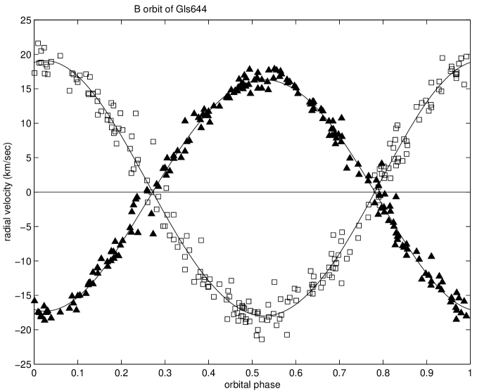
Figure 4: The radial-velocity curve for the inner orbit. The motion of the center of mass of the B system around A has been removed from the velocities plotted for Ba and Bb, represented by filled triangles and open squares, respectively.

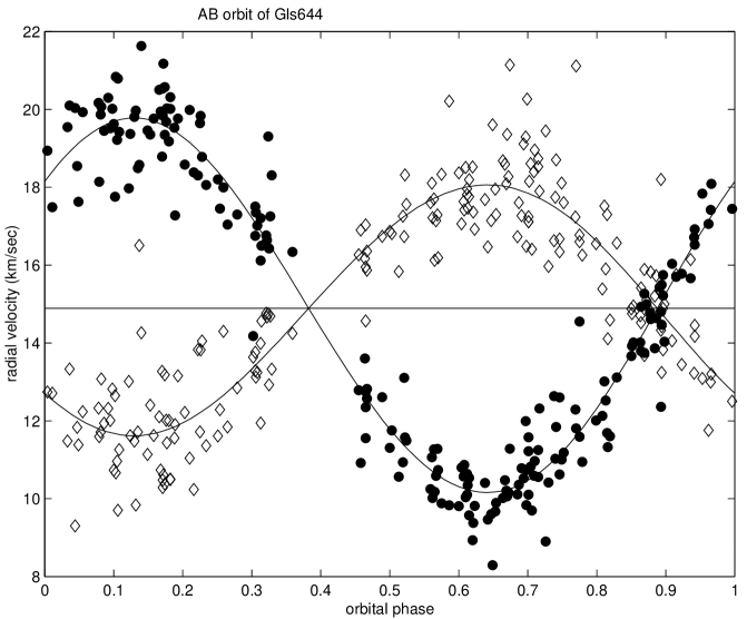
Figure 5: The radial-velocity curve for the outer orbit. The velocities observed for A are plotted as filled circles, and open diamonds are used for the average velocity of Ba and Bb, weighted according to their mass ratio.

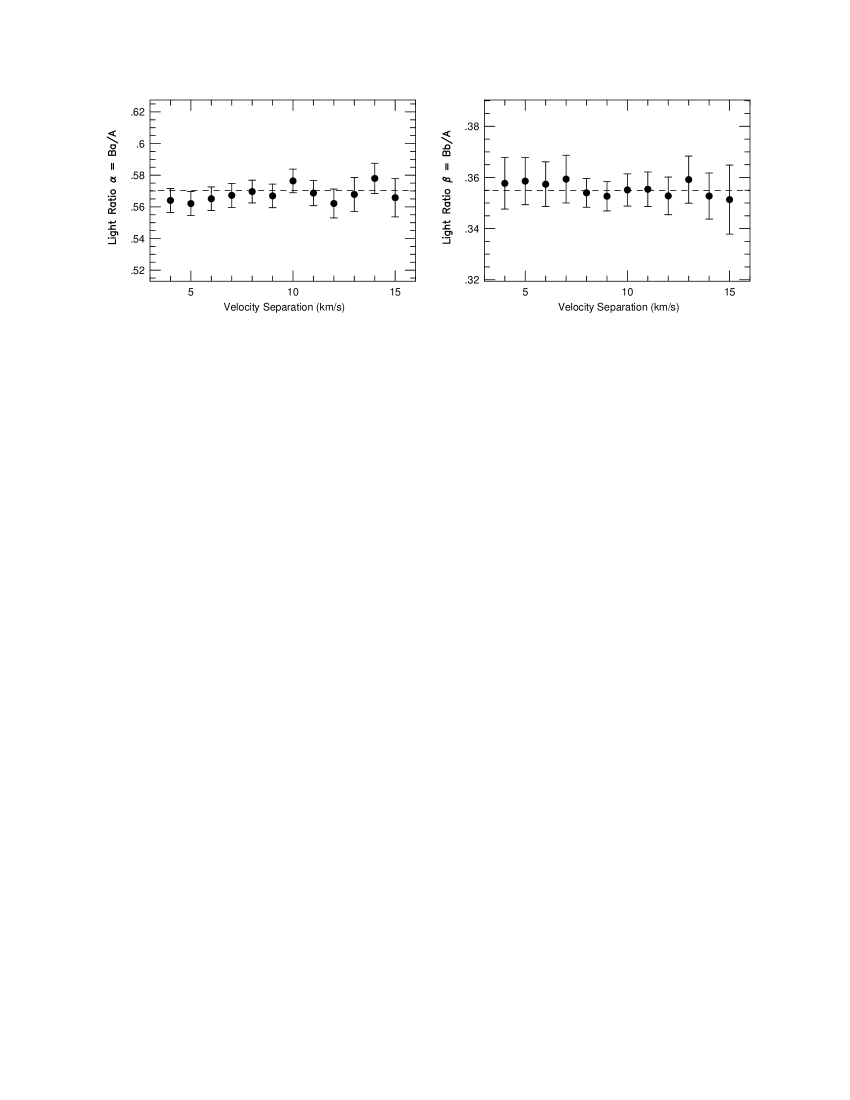
Figure 6: The light ratios $\alpha$ and $\beta$ from the CfA analysis as a function of the minimum velocity separation between any two components of the Gliese 644 system.

For each iteration in the CfA analysis we used the orbital solution from the previous iteration to provide TODCOR with initial values for the velocities of the three stars. We then allowed TODCOR to search for the nearest peak in correlation space. This procedure should eliminate or at least minimize the cases where TODCOR finds the wrong correlation peak and assigns an incorrect velocity to one or more of the stars. Therefore, for the CfA analysis we chose not to swap any of TODCOR’s velocity assignments. The orbital solution was carried out with an independent code that solves simultaneously for all elements of the inner and outer orbits, by computing differential corrections to a set of initial elements. The results are reported in Table 5, and the (O-C) residuals of the individual velocities from this solution are listed in Table 4.

3.3 The adopted spectroscopic orbits

The agreement between the Tel Aviv and CfA analyses of the spectroscopic orbits is satisfactory for all of the orbital parameters except the velocity amplitudes for the outer orbit, $K_{\mathrm{A}}$ and $K_{\mathrm{B}}$, and the center-of-mass velocity, $\gamma$, where the differences exceed three times the combined internal error estimates. These differences lead to a relatively large difference in the mass ratio $q_{\mathrm{AB}}=K_{\mathrm{A}}:K_{\mathrm{B}}$, which we use to divide up the total mass from the astrometric orbit in the next section. Apparently there is a systematic error lurking in one or both of our analyses, but we have not been able to identify the culprit. Therefore we have chosen to adopt final orbital parameters that are simply the average of the values from the two solutions, as reported in Table 5. For the final errors we adopted half the difference between the two solutions, or the average of the two internal error estimates, whichever was larger.

The agreement between the astrometric orbit and our adopted spectroscopic orbit is well within the errors, which are much smaller for the astrometric solution. By convention, the longitude of periastron for an astrometric orbit refers to the secondary, but for a spectroscopic orbit it refers to the primary. After this difference of $180\degr$ is taken into account, the values for $\omega$ agree well.

4 THE MASSES AND ORBITAL INCLINATIONS OF GLIESE 644

4.1 The masses of the three stars

The combination of spectroscopic orbits for the inner and outer binaries together with an astrometric orbit for the outer visual binary enables us to derive masses for all three components of Gliese 644. The total mass of the system can be derived from the parallax together with the dynamical quantity $(a^{3}/P^{2})$ provided by the astrometric solution. The individual masses can then be deduced using the two mass ratios derived from the spectroscopic solutions.

For the parallax we note that the Fourth Edition of the General Catalog of Trigonometric Parallaxes (van Altena, Lee & Hoffleit 1995) gives the weighted average of 16 determinations as $\pi_{\rm trig}=0\thinspace\aas@@fstack{\prime\prime}1548\pm 0\thinspace\aas@@fstack{\prime\prime}0006$. The Hipparcos catalog (ESA 1997) lists a considerably larger value ($\pi_{\rm HIP}=0\thinspace\aas@@fstack{\prime\prime}1742\pm 0\thinspace\aas@@fstack{\prime\prime}0039$), which is almost certainly affected by the 1.7-yr orbital motion of the visual pair. Söderhjelm (1999) took this orbital motion into account in his reanalysis of the Hipparcos data and derived $\pi=0\thinspace\aas@@fstack{\prime\prime}1556\pm 0\thinspace\aas@@fstack{\prime\prime}0018$, in excellent agreement with the ground-based value. These determinations are plotted in Figure 7, including the 16 individual ground-based values. A valuable check is provided by Gliese 643, which is a common-proper-motion companion to Gliese 644 and is therefore expected to be at the same distance (see Section 7). The value of its parallax as measured by Hipparcos is $\pi_{\rm HIP}=0\thinspace\aas@@fstack{\prime\prime}1540\pm 0\thinspace\aas@@fstack{\prime\prime}0040$, again in good agreement with the ground-based value for Gliese 644. We adopt the ground-based value for the parallax of Gliese 644 because it has the smallest estimated error.

Figure 7: Parallax determinations for Gliese 644. The individual ground-based results are plotted as circles. The weighted average is indicated by the dotted line. The arrow points to the corresponding error bar. Söderhjelm’s (1999) redetermination for Gliese 644 is plotted as a filled square, replacing the Hipparcos value plotted as an open square.

Combining $(a^{3}/P^{2})$ from our adopted astrometric orbit with the parallax we get that the total mass is

$$M_{\mathrm{tot}}=\frac{(a^{3}/P^{2})}{\pi^{3}}=1.049\pm 0.020\ (1.9\%)\ {M_{\odot}}\,.$$ (1)

An alternative way to derive the semi-major axis of the wide binary, and consequently the total mass of the system, is to use the radial-velocity amplitudes derived from the spectroscopy together with the inclination angle derived from the astrometry. This yields $M_{\mathrm{tot}}=1.17\pm 0.40{M_{\odot}}$. Note that the error for this approach is an order of magnitude larger than the one corresponding to the mass derived from the astrometry alone, and the total masses from the two approaches agree within this large error.

The mass ratios given by our adopted spectroscopic orbits are $q_{\mathrm{B}}=M_{\mathrm{Bb}}:M_{\mathrm{Ba}}=0.906\pm 0.015$ for the inner orbit and $q_{\mathrm{AB}}=M_{\mathrm{B}}:M_{\mathrm{A}}=1.56\pm 0.17$ for the outer orbit. Combining these mass ratios with the definitions $M_{\mathrm{tot}}=M_{\mathrm{A}}+M_{\mathrm{B}}$ and $M_{\mathrm{B}}=M_{\mathrm{Ba}}+M_{\mathrm{Bb}}$, we conclude that

$$M_{\mathrm{A}}=\frac{1}{(1+q_{\mathrm{AB}})}M_{\mathrm{tot}}=0.410\pm 0.028\ (6.9\%)\ {M_{\odot}}\,,$$ (2)

$$M_{\mathrm{Ba}}=\frac{q_{\mathrm{AB}}}{(1+q_{\mathrm{B}})(1+q_{\mathrm{AB}})}M_{\mathrm{tot}}=0.336\pm 0.016\ (4.7\%)\ {M_{\odot}}\,,$$ (3)

$$M_{\mathrm{Bb}}=\frac{q_{\mathrm{B}}q_{\mathrm{AB}}}{(1+q_{\mathrm{B}})(1+q_{\mathrm{AB}})}M_{\mathrm{tot}}=0.304\pm 0.014\ (4.7\%)\ {M_{\odot}}.$$ (4)

These values are similar to the ones found by Söderhjelm (1999), who derived $M_{\mathrm{A}}=0.41\pm 0.04$ and $M_{\mathrm{B}}=0.66\pm 0.06{M_{\odot}}$, and to the ones derived by Ségransan et al. (2001), who obtained masses of $0.4155\pm 0.0057$, $0.3466\pm 0.0047$ and $0.3143\pm 0.0040$, for the masses of $A$, $Ba$ and $Bb$, respectively.

4.2 The orbital inclinations

We can now go back and calculate the inclinations of the two orbits relative to our line of sight, using the spectroscopic values for $M\sin^{3}i$ adopted in Table 5, together with the individual masses derived in the previous section. We get

$$i_{AB}=17\aas@@fstack{\circ}4\pm 1\aas@@fstack{\circ}4\ {\rm or}\ 162\aas@@fstack{\circ}6\pm 1\aas@@fstack{\circ}4,\ \ \ i_{B}=16\aas@@fstack{\circ}3\pm 0\aas@@fstack{\circ}3\ {\rm or}\ 163\aas@@fstack{\circ}7\pm 0\aas@@fstack{\circ}3\,.$$ (5)

The ambiguity comes from the fact that the radial-velocity data can not specify whether the orbital motions are retrograde or direct. The inclination of the outer orbit from the astrometric solution, $i_{AB}=163\aas@@fstack{\circ}1\pm 1\aas@@fstack{\circ}6$, is close to the retrograde value from the spectroscopic orbit.

The inclinations of the two orbits do not provide enough information to derive the relative angle between the two orbits, $\phi$, which can be written as (Mazeh & Shaham 1976):

$$\cos\phi=\cos i_{\mathrm{B}}\cos i_{\mathrm{AB}}+\sin i_{\mathrm{B}}\sin i_{\mathrm{AB}}\cos(\Omega_{\mathrm{B}}-\Omega_{\mathrm{AB}})\,,$$ (6)

where $\Omega_{\mathrm{B}}$ and $\Omega_{\mathrm{AB}}$ are the position angles of the line of nodes of the inner and outer orbits, respectively. Since $\Omega_{\mathrm{B}}$ is unknown, we can only limit $\phi$ (Batten 1973):

$$i_{\mathrm{A}}-i_{\mathrm{AB}}\leq\phi\leq i_{\mathrm{A}}+i_{\mathrm{AB}},$$ (7)

which in our case results in

$$1\aas@@fstack{\circ}1\pm 1\aas@@fstack{\circ}4\leq\phi\leq 33\aas@@fstack{\circ}7\pm 1\aas@@fstack{\circ}4\,.$$ (8)

Equation (8) implies that the relative angle between the two orbits could be as large as $34\degr$. However, to make the two inclinations come out so close requires a special orientation. It is more natural to suppose that the two orbits really are almost coplanar.

5 PHOTOMETRY

The Hipparcos Catalogue lists $V=9.02$ mag for the total combined light of Gliese 644, while SIMBAD cites 6 determinations that lead to $V=9.02\pm 0.01$ mag. To divide the total light between the three components we use the adopted values of the spectroscopic light ratios at 5187 Å derived by TODCOR, $\alpha=0.569\pm 0.034$ and $0.358\pm 0.024$. After the application of small corrections to move these light ratios to 5550 Å, the value we adopted for the effective wavelength of the $V$ band, these ratios become $0.576\pm 0.034$ and $0.364\pm 0.024$. Dividing the $V$ brightness with these light ratios, and applying our adopted parallax of $\pi=0\thinspace\aas@@fstack{\prime\prime}1548\pm 0\thinspace\aas@@fstack{\prime\prime}0006$, we find that $M_{V}\mathrm{(A)}=10.69\pm 0.02$, $M_{V}\mathrm{(Ba)}=11.29\pm 0.05$, and $M_{V}\mathrm{(Bb)}=11.79\pm 0.05$ mag.

As a check on the spectroscopic light ratios derived with TODCOR, we calculate the total light that those ratios predict for the B subsystem and compare it with the magnitude difference between A and B found by others. The simple average of the 70 visual magnitude differences reported in the Washington Double Star Catalog (Worley & Douglass 1996) gives $0.103\pm 0.014$. Söderhjelm (1999) reports a difference in the Hipparcos magnitudes of 0.11 based on his reanalysis of the Hipparcos data. These magnitude differences are both consistent with our result that the total light of B is fainter than A by $0.07\pm 0.05$ mag in the $V$ band.

The three new speckle observations reported in this paper provide infrared magnitude differences, and show that B is brighter than A at $J$, $H$, and $K$ by $0.51\pm 0.01$, $0.56\pm 0.02$, and $0.66\pm 0.06$ mag, respectively. The fact that B is fainter than A in the visual but brighter in the infrared is qualitatively consistent with the fact that the two components of B are cooler than A.

However, when we use our derived masses to predict the magnitudes expected for A and B in detail, a problem emerges. This is illustrated in Figure 8a, where we plot the observed absolute magnitudes for A (tesselated stars) and B (filled triangles) at $V$, $J$, $H$, and $K$, using the apparent magnitudes for Gliese 644 (all three stars together) of $J=5.37$, $H=4.67$, and $K=4.38$. We used Leggett (1992) observations and applied small corrections to convert them to the Johnson system. We also plot the predicted absolute magnitudes as a function of wavelength from 5 Gyr solar-metallicity models (solid lines, Baraffe et al. 1998) and [Fe/H] = $-0.5$ metal-poor models (dash-dotted lines, Baraffe et al. 1997). In both cases the lower line of each pair corresponds to the prediction for A, and the upper line for B. The infrared absolute magnitudes predicted for A are slightly brighter than observed, while the corresponding predictions for B are typically too faint. In the visual band, the solar-metallicity model is slightly too bright for both stars.

Figure 8: Absolute magnitudes (panel a) and magnitude differences (panel b) for Gliese 644 A and B. In panel a the observed A magnitudes are denoted by stars, and those of B by triangles. The predicted absolute magnitudes for A and B from 5 Gyr solar-metallicity models are shown as solid lines, and from [Fe/H] = $-0.5$ metal-poor models as dash-dotted lines. In panel b a 0.1 Gyr solar-metallicity prediction is plotted as a dashed line. The plus signs present the magnitude differences predicted by the Henry & McCarthy (1993) empirical mass-luminosity relations.

These discrepancies become more obvious when we plot the magnitude differences (B$-$A), as shown in panel b. The 5 Gyr solar-metallicity and [Fe/H] = $-0.5$ metal-poor model predictions are again plotted as solid and dash-dotted lines, respectively, while a 0.1 Gyr solar-metallicity prediction is plotted as a dashed line. Although metallicity and age both have some effect on the predicted magnitude differences, the effect is much smaller than the discrepancy with the observed magnitude differences. To show that the models appear to be reliable, we plot (as plus signs) the magnitude differences predicted by the Henry & McCarthy (1993) empirical mass-luminosity relations. We are puzzled by these discrepancies and see no easy explanation.

6 THE MASS-LUMINOSITY RELATION AND GLIESE 644

The individual masses that we have derived for the three M dwarfs in the Gliese 644 system have formal errors of 5 to 7 %, which puts these results into a category with only a dozen or so stars that have masses smaller than 0.6 $M_{\odot}$ and mass uncertainties similar or better than ours. At this level of accuracy we can begin to make meaningful tests of the theoretical models for low-mass stars.

It has been traditional to assess the mass-luminosity relation using the absolute $V$ magnitude versus mass diagram. We can plot all three stars in the Gliese 644 system on this diagram, because TODCOR has provided us with the spectroscopic light ratios needed to divide up the light between the two components of the unresolved inner binary at a wavelength close to the V band. Thus we use the $M_{V}$ versus mass diagram to assess the present status of the confrontation between the observations and the Baraffe et al. (1997, 1998) theoretical isochrones for low-mass stars.

Table 6: Lower main-sequence stars with mass and V absolute magnitude better than 5%.

Star	Mv	Mass	Ref.
Gls 791.2 A	13.38 $\pm$ 0.03	0.2866 $\pm$ 0.0061	Benedict et al. 2000
Gls 791.2 B	16.65 $\pm$ 0.10	0.1258 $\pm$ 0.0029
Gls 860 A	11.81 $\pm$ 0.07	0.2570 $\pm$ 0.011	Henry & McCarthy 1993
Gls 860 B	13.39 $\pm$ 0.06	0.1720 $\pm$ 0.008	Henry et al. 1999
GJ 2069 A	11.70 $\pm$ 0.2	0.4329 $\pm$ 0.0018	Delfosse et al. 1999a
GJ 2069 B	12.45 $\pm$ 0.2	0.3975 $\pm$ 0.0015
Gls 866 A	15.34 $\pm$ 0.14	0.1216 $\pm$ 0.0029	Delfosse et al. 1999b
Gls 866 B	15.58 $\pm$ 0.07	0.1161 $\pm$ 0.0029
Gls 866 C	17.34 $\pm$ 0.45	0.0957 $\pm$ 0.0023
YY Gem A	8.99 $\pm$ 0.08	0.5880 $\pm$ 0.022	Andersen 1991
YY Gem B	8.99 $\pm$ 0.08	0.5880 $\pm$ 0.022
CM Dra A	12.75 $\pm$ 0.04	0.2307 $\pm$ 0.0010	Metcalfe et al. 1996
CM Dra B	12.90 $\pm$ 0.04	0.2136 $\pm$ 0.0010
Gls 644 A	10.69 $\pm$ 0.02	0.410 $\pm$ 0.028	This paper
Gls 644 Ba	11.29 $\pm$ 0.05	0.336 $\pm$ 0.016
Gls 644 Bb	11.79 $\pm$ 0.05	0.304 $\pm$ 0.014

In Table 6 we list the masses and absolute visual magnitudes obtained here for Gliese 644, as well as data for other stars below 0.6 $M_{\odot}$ with uncertainties in the masses smaller than 5%, which we take as a benchmark for comparison. These measurements are shown in Figure 9. We did not list and plot Gliese 570 BC (Forveille et al. 1999) because that close system has not been resolved in the visual, and therefore observed $V$ magnitudes are not available for the two components.

Figure 9: The mass-luminosity relation for stars on the lower main sequence with mass determinations more accurate than 5%. The three components of Gliese 644 are plotted as tesselated stars. For comparison we also show the determinations for Gliese 644 by Ségransan et al. (2001). The components of the three eclipsing binaries YY Gem, GJ 2069A, and CM Dra are plotted as filled circles, and the components of the astrometric systems Gliese 860, Gliese 866, and Gliese 791.2 as open circles. The solid line is the solar-metallicity 5 Gyr isochrone, and the dashed line is the metal-poor 5 Gyr isochrone with [Fe/H] = $-0.5$. The corresponding 10 Gyr isochrones are plotted as dotted lines.

In the figure we plot solar-metallicity 5 Gyr isochrone from Baraffe et al. (1998), and metal-poor 5 Gyr isochrone with [Fe/H] = $-0.5$ from Baraffe et al. (1997). The corresponding 10 Gyr isochrones are also plotted. As can be seen from the figure, some of the observed points are far off from both theoretical lines.

Forveille et al. (1999) suggest that the Baraffe et al. models (1997, 1998) may be missing some opacity sources, and that the solar-metallicity isochrones should be lower than they appear in Figure 9. This might produce better agreement with the observed results for CM Dra, Gliese 866 and 860, in which case the good agreement of our three points for Gliese 644 might imply that the system is slightly metal poor and/or very young. Can the much more serious discrepancies for GJ 2069A, as suggested by Delfosse et al. (1999a), and for Gliese 791.2, be explained by extreme metal richness? The answer to this question will have to wait for the calculation of theoretical isochrones for super-metal-rich models and for the observational determination of accurate metallicities for these stars. In the meantime we must conclude that the mass-luminosity relation near the bottom of the main sequence is still not well understood, at least in the visual band. Note that the above dicussion did not take into account the possiblity of stellar spots, which could affect the stellar luminosity. In the future, it might be better to move to infrared magnitudes, where the effects of stellar spots on the photometry are less severe.

Figure 9 shows that changing the stellar age from 5 to 10 Gyr has no significant effect on the theoretical isochrones for stars less massive than about 0.5 $M_{\odot}$. However, changing the metallicity from [Fe/H] = 0.0 to $-0.5$ has a large effect. To allow a meaningful confrontation between the models and the observations in the $M_{V}$ versus mass diagram, it is necessary to have accurate metallicities for the stars involved, good to 0.1 in [Fe/H] or better. Otherwise, the metallicity uncertainties are likely to dominate the uncertainties from the photometry, parallaxes, and masses. Unfortunately, accurate metallicity determinations are still beyond the state of the art for stars near the bottom of the main sequence. Of all the systems plotted in Figure 9, for example, only for CM Dra has the metallicity been analyzed in some detail, with ambiguous results (Viti et al. 1998). They find that CM Dra may be somewhat metal poor, which would be consistent with its unusually high space motion, or it may have almost solar metallicity, but it is unlikely to be metal rich.

Actually, it is possible that metallicity alone is not enough to understand the mass-luminosity relation. For example, it may turn out that it is not valid to assume that the helium abundance scales with the metallicity, in which case it will also be necessary to determine the bulk helium abundance. Stellar age is certainly another factor that can change the stellar luminosity. We expect therefore that studies of stars in clusters will (continue to) be important for progress in testing stellar models, because additional information about the age and metallicity can be derived for cluster stars.

7 THE DISTANT COMPANIONS OF GLIESE 644

In this section we discuss two additional stars associated with the Gliese 644 triple system. One of them is Gliese 643 (=Wolf 629, $\alpha=16$:55:25.26, $\delta=-8$:19:21.3 [J2000], $V=11.74$ mag), at a projected separation of about $70\arcsec$ from Gliese 644. The other companion, at a separation of $220\arcsec$, is the faint star vB 8 (=Gliese 644C, $\alpha=16$:55:35.74, $\delta=-08$:23:36.0 [J2000], $V=16.80$ mag). The common proper motion of Gliese 644 and 643 (Wolf 1919) and their similar parallax (e.g., ESA 1997) strongly indicate that they are indeed physically connected. Van Biesbroeck (1961) found that vB 8 also shares with Gliese 644 the same proper motion, attesting to its physical association with the system.

vB 8 (spectral type M7.0 V) and vB 10 (M8.0 V), a companion to Gliese 752 also found by van Biesbroeck, were long considered to represent the bottom of the stellar main sequence. Although many cooler and less luminous objects are now known, vB 8 is still of interest, because its mass must be very near the substellar limit of 0.08 $M_{\odot}$. Using the updated mass-luminosity relation of Henry et al. (1999), we derive from the $M_{V}$ values of Gliese 643 and vB 8 (12.69 and 17.75 mag) mass estimates of 0.19 and 0.08 $M_{\odot}$, respectively.

Joy (1947, see Abt 1973) obtained a few spectra of Gliese 643 and reported that its radial velocity was variable. Since that time Gliese 643 has usually been reported in the literature as a spectroscopic binary (e.g., Eggen 1978, Johnson 1987). To follow its orbital motion, we secured 83 spectra of Gliese 643, spread over 5843 days, but could not find any significant radial-velocity variation. Our velocities, derived using Gliese 725B as the template, have an r.m.s of 0.63 km s^-1, slightly larger than our typical errors for M dwarfs, and the $\chi^{2}$ probability is small, but we can not find any periodicity in the velocities or any orbital solution that pass our usual tests for being significant. If Gliese 643 is a spectroscopic binary, the orbital amplitude must be less than about 0.5 km s^-1. Our individual velocities for Gliese 643 are reported in Table 7.

Table 7: Radial velocities and internal error estimates (km s^-1) for Gliese 643 (first 20 lines)

HJD	$V_{\rm{r}}$	$\sigma_{\rm{int}}$
2445780.9993	16.44	$\pm 0.41$
2446511.9753	15.84	$\pm 0.26$
2446512.8511	15.82	$\pm 0.45$
2446513.8675	15.87	$\pm 0.59$
2446520.0150	15.94	$\pm 0.33$
2446520.8916	16.00	$\pm 0.85$
2446523.8416	15.78	$\pm 0.39$
2446537.9360	15.73	$\pm 0.20$
2446538.9771	16.22	$\pm 0.26$
2446539.8486	15.79	$\pm 0.60$
2446540.8417	15.03	$\pm 0.32$
2446540.9364	15.83	$\pm 0.21$
2446541.8916	15.17	$\pm 0.22$
2446565.7301	15.42	$\pm 0.43$
2446568.7910	15.97	$\pm 0.34$
2446569.6356	15.75	$\pm 0.79$
2446569.7865	15.58	$\pm 0.53$
2446569.7964	16.27	$\pm 0.59$
2446608.6348	15.54	$\pm 0.94$
2446612.7619	14.80	$\pm 0.69$

The mean radial velocity we find for Gliese 643 is $15.81\pm 0.07$ km s^-1on the CfA system, i.e. with the same zero point as the CfA velocities for Gliese 644. This is very close to the center-of-mass velocity of Gliese 644, $\gamma=15.10\pm 0.21$. The projected separation between Gliese 644 and 643 is about 450 AU, which corresponds to an orbital velocity of about 1.5 km s^-1 for a circular orbit. The observed velocity difference is only 0.7 km s^-1, consistent with the interpretation that Gliese 643 is gravitationally bound in an orbit with Gliese 644.

We have also secured one low S/N spectrum of vB 8 with the Digital Speedometer on the MMT and found its radial velocity to be $15.68\pm 1.09$ km s^-1, consistent with the interpretation that vB 8 is bound to the Gliese 643/644 system in a hierarchical quintuple configuration. In this picture vB 8 moves around the center of mass of the Gliese 644/643 system.

The projected separation between vB 8 and Gliese 644 is only three times larger than the projected separation between Gliese 643 and Gliese 644. Such a small ratio usually renders triple systems dynamically unstable (e.g., Eggelton & Kiseleva 1995, Kiseleva et al. 1995). Therefore, we suggest that the actual separation between vB 8 and Gliese 644 is significantly larger than its projected separation, by at least a factor of two.

8 ON THE FORMATION AND EVOLUTION OF THE SYSTEM

Our picture of the Gliese 644/643/vB 8 system can be summarized as follows:

• All five stars reside in an hierarchical system. The orbital sizes are of the order of 2000 (projected), 500 (projected), 1 and 0.05 AU for vB 8, Gliese 643, Gliese 644AB, and Gliese 644B, respectively.

• The masses of vB 8, Gliese 643, Gliese 644A/Ba/Bb are of the order 0.1, 0.2, 0.4, 0.3, 0.3 $M_{\odot}$, respectively.

• The innermost two orbits, in the Gliese 644 system itself, are probably coplanar.

In this section we briefly discuss two extremely simplistic scenarios for the formation and evolution of the system. First we consider a scenario in which the quintuple was formed by a sequence of fragmentation events during the collapse of a molecular cloud core (e.g., Burkert & Bodenheimer 1993) leading directly to the hierarchical configuration now observed. The cloud core collapsed until it was a few thousand AU in diameter, at which point it fragmented into three parts. The two smaller parts ended up as vB 8 and Gliese 643. The larger fragment continued to contract by another three orders of magnitude, until a hydrostatic core was formed with a radius of a few AU (e.g., Larson 1969). When the temperature of the core reached about 2000 K the molecular hydrogen began to dissociate, resulting in a second collapse within the hydrostatic core (e.g. Larson 1969). During the second collapse the core may have been able to fragment again into the components of the visual binary, Gliese 644A and Gliese 644B, the latter of which fragmented again into Ba and Bb.

This scenario is not free of some problems. Although fragmentation calculations have successfully simulated the formation of wide binaries during the collapse of molecular cloud cores, there is still some uncertainty about whether or not this step can succeed in forming a stable binary with separation as small as 1 AU (e.g., Boss 1989, Bonnell & Bate 1994, Bate 1998). Moreover, there have not yet been successful fragmentation calculations for the formation of very close binaries, such as Gliese 644B with a separation of only 0.05 AU. Whatever mechanism was responsible for the formation of Gliese 644B system, it is interesting that the mass ratio for this binary is close to unity, a mass ratio which is apparently quite frequent in spectroscopic binaries (Tokovinin 2000). A mechanism that can lead, under the right conditions, to nearly equal masses in a close binary has been studied by Bate & Bonnell (1997) and Bate (2000). Initially, two stellar seeds form, with masses at most a few percent of the final stellar masses. Most of the mass of the collapsing cloud core is still in a gaseous envelope surrounding the seeds. The accretion of material onto the seeds then builds the masses up to the final stellar values. The smaller of the two seeds is favored in the amount of mass that it receives, and this tends to equalize the masses of the final components of the binary, after the envelope material has been exhausted.

If the two orbits in the Gliese 644 system are coplanar, as suggested by our spectroscopic results, then this might lend support to fragmentation as the formation mechanism for the innermost binary; it is natural to suppose that the two orbital planes for Gliese 644 should both be oriented perpendicularly to the angular momentum vector of the molecular cloud core from which they formed.

Dynamical evolution in a small-N cluster (e.g., McDonald & Clarke 1993, 1995) is another possible scenario for the formation of the Gliese 644/643/vB 8 system. In this scenario all five stars were formed independently within a loosely self-gravitating small-N cluster of stars. Gravitational interactions between the cluster members then evolved the orbits of the five stars, the ones we see now, into a hierarchical configuration, while ejecting the other stars from the cluster. In this scenario, the more massive stars are expected to settle into more tightly bound orbits, while the less massive stars are raised into less tightly bound orbits, just as is observed for the system. However, this scenario does not easily account for the coplanarity of the Gliese 644 triple, a feature often found in other triple systems as well (Fekel 1981, Tokovinin 1997).

Another possible way to explain the coplanarity of the close triple Gliese 644 involves tidal interactions. It is well known that a large relative inclination between the two orbits of a triple can induce strong oscillations of the inner eccentricity (e.g., Mazeh, Krymolowski & Rosenfeld 1997), which can make the system dynamically unstable. Therefore, the low relative inclination of the two orbits in the Gliese 644 triple might be the result of some selective evolutionary process. Triple systems with large relative inclinations simply could not survive. This argument still has to be worked out, though, because the amplitude of the eccentricity modulation does not depend linearly on the relative inclination (e.g., Holman, Touma & Tremaine 1997), and there are medium-sized angles, on the order of 10–20 degrees, that do not produce large eccentricity modulations.

A potentially interesting feature of the Gliese 644 triple — the very marginal evidence for a minute variation of the outer orbit’s eccentricity — might also be a result of tidal interactions (Mazeh & Shaham 1979, Paper II). A few spectroscopic triple systems have already been observed to display direct or indirect evidence for long-term tidal modulations (Mayor & Mazeh 1987, Mazeh 1990, Jha et al. 1997), of which HD 109486 is the best example (Jha et al. 2000). Right now the effect observed in Gliese 644 is much too marginal to rely on. Many more years of observations will be needed to see if the effect is real.

The Gliese 644/643/vB 8 system is the nearest known quintuple stellar system. The next nearest system with five or more objects is Castor (=Gliese 278) at 16 pc (Tokovinin 1999). In order to better understand how multiple systems of low-mass stars form and evolve, it would be extremely interesting to find more M-star multiple systems in the solar neighborhood and to compare their features. In this vein, it is amazing that another triple M-star system exhibits very similar features to Gliese 644. This is Gliese 866, which was recently studied by Delfosse et al. (1999b) and by Woitas et al. (2000). Delfosse et al. derived the two orbital periods, of 803 and 3.78 days, and masses of 0.12, 0.11 and 0.096 $M_{\odot}$. Woitas et al. (2000) derived a period of 821 days for the outer orbit. Although the masses in the Gliese 644 triple are almost three times larger, in both systems there are three M stars with similar masses, where the most massive star is 30% more massive than the lightest one, and the period ratio is slightly larger than 200. Moreover, both systems are probably very close to coplanar. One wonders if these features are common in M-star triples.

References

- [1] Abt, H. A., 1973, ApJS, 26, 365
- [2] Andersen, J., 1991, A&AR, 3, 91
- [3] Baraffe, I., Chabrier, G., Allard, F., Hauschildt, P. H., 1997, A&A, 327, 1054
- [4] Baraffe, I., Chabrier, G., Allard, F., Hauschildt, P. H., 1998, A&A, 337, 403
- [5] Bate. M. R., 1998, ApJ, 508, L95
- [6] Bate, M. R., 2000, MNRAS, 314, 33
- [7] Bate, M. R., Bonnell, I. A., 1997, MNRAS, 285, 33
- [8] Batten, A., 1973, Binary and Multiple Star Systems, Pergamon Press, Oxford, p. 73
- [9] Benedict, G. F., McArthur, B. E., Franz, O. G., Wasserman, L. H., Henry, T. J., 2000, AJ, 120, 1106
- [10] Bonnell, I. A., Bate, M. R., 1994, MNRAS, 271, 999
- [11] Boss, A. P., 1989, ApJ, 346, 336
- [12] Burkert, A., Bodenheimer, P., 1993, MNRAS, 264, 798
- [13] Delfosse, X., Forveille, T., Mayor, M., Burnet, M., Perrier, C., 1999a, A&A, 341L, 63
- [14] Delfosse, X., Forveille, T., Udry, S., Beuzit, J.-L., Mayor, M., Perrier, C., 1999b, A&A, 350L, 39
- [15] Douglass, G. G., & Worley, C. E., 1992, in McAlister, H. A., Hartkopf, W. I., eds, ASP Conf. Ser. 32, IAU Coll. 135, Complementary Approaches to Double and Multiple Star Research, Astron. Soc. Pac., San Francisco, p. 311
- [16] Eggen, O. J., 1978, ApJ, 226, 405
- [17] Eggleton, P., Kiseleva, L., 1995, ApJ, 455, 640.
- [18] ESA, 1997, The Hipparcos and Tycho Catalogues, European Space Agency, SP-1200, ESA Publications Division, ESTEC, Noordwijk, The Netherlands
- [19] Fekel, F. C., 1981, ApJ, 246, 879
- [20] Fleischer, R., 1957, Astron. J., 62, 379
- [21] Forveille, T., Beuzit, J., Delfosse, X., Ségransan, D., Beck, F., Mayor, M., Perrier, C., Tokovinin, A., Udry, S., 1999, A&A, 351, 619
- [22] Gliese, W., 1969, Veröff. Astron. Rechen-Inst. Heidelberg No. 22
- [23] Goldberg, D., Mazeh, T., Latham, D. W., Stefanik, R. P. Carney, B. W., Laird, J. B., 2000, submitted to AJ
- [24] Heintz, W. D., 1984, PASP, 96, 439
- [25] Henry, T. J., 1991, PhD thesis, University of Arizona
- [26] Henry, T. J., Kirkpatrick, J. D., Simons, D. A., 1994, AJ, 108, 1437
- [27] Henry, T. J., McCarthy, D. W., Jr. 1993, AJ, 106, 773
- [28] Henry, T. J., Franz, O. G., Wasserman, L. H., Benedict, G. F., Shelus, P. J., Ianna, P. A., Kirkpatrick, J. D., McCarthy, D. W., Jr., 1999, ApJ, 512, 864
- [29] Holman, M., Touma, J., Tremaine, S., 1997, Nature, 386, 254 M. J., 1997, AJ, 113, 1915
- [30] Jha, S., Torres, G., Stefanik, R. P., Latham, D. W., 1997, Baltic Astronomy, 6, 55
- [31] Jha, S., Torres, G., Stefanik, R. P., Latham, D. W., Mazeh, T., 2000, MNRAS, 317, 375, Paper III
- [32] Johnson, H. M., 1987, ApJ, 316, 458
- [33] Joy, A. H., 1947, ApJ, 105, 96
- [34] Kiseleva, L., Anosova, J., Eggleton, P., Cohn, J., Orlov, V., 1995, in van der Kruit, P. C. Gilmore, G. eds, IAU Symp. 164, Stellar Populations, Kluwer Academic Publishers, Dordrecht, p. 370
- [35] Krymolowski, Y., Mazeh, T., 1999, MNRAS, 304, 720, paper II
- [36] Kuiper, G. P., 1934, PASP, 46, 235
- [37] Larson, R. B., 1969, MNRAS, 145, 271
- [38] Latham, D. W., 1985, in Philip, A. G. D., Latham, D. W., eds, IAU Coll. 88, Stellar Radial Velocities, L. Davis Press, Schenectady, NY, p. 21
- [39] Latham, D. W. 1992, in H. McAlister, H., Hartkopf, W., eds, ASP Conf. Ser. 32, IAU Coll. 135, Complementary Approaches to Binary and Multiple Star Research, Astron. Soc. Pac., San Francisco, p. 110
- [40] Leggett, S. K., 1992, ApJS, 82, 351
- [41] Mayor, M., Mazeh, T., 1987, A&A, 171, 157
- [42] Mazeh, T., 1990, AJ, 99, 675
- [43] Mazeh, T., Zucker, S., Goldberg, D., Latham, D. W., Stefanik, R. P., Carney, B. W., 1995, ApJ, 449, 909
- [44] Mazeh, T., Krymolowski, Y., Latham, D. W., 1993, MNRAS, 263, 775, paper I
- [45] Mazeh, T., Krymolowski, Y., Rosenfeld, G., 1997, ApJ, 477, L103
- [46] Mazeh, T., Shaham, J., 1976, ApJ, 205, L147
- [47] Mazeh, T., Shaham, J., 1977, ApJ, 213, L17
- [48] Mazeh, T., Shaham, J., 1979, A&A, 77, 145
- [49] McCarthy, D. W., Jr. 1986, in Kafatos, M. C., Harrington, R. S., Maran, S. P., eds, Astrophysics of Brown Dwarfs, Cambridge Univ. Press, Cambridge, p. 9
- [50] McCarthy, D. W., Jr., Henry, T. J., McLeod, B. A., Christou, J. C., 1991, AJ, 101, 214
- [51] McDonald, J. M., Clarke, C. J., 1993, MNRAS, 262, 800
- [52] McDonald, J. M., Clarke, C. J., 1995, MNRAS, 275, 671
- [53] Metcalfe, T. S., Mathieu, R. D., Latham, D. W., Torres, G., 1996, ApJ, 456, 356
- [54] Nordström, B., Latham, D., Morse, J. A., Milone, A. A. E., Kurucz, R. L., Andersen, J., Stefanik, R. P., 1994, A&A, 287, 338
- [55] Pannunzio, R., Zappala, V., Massone, G., & Morbidelli, R., 1986, A&A, 166, 337
- [56] Press, W. H., Teukolsky, S. A., Vetterling, W. T., Flannery, B. P., 1992, Numerical Recipes, 2nd Ed., Cambridge Univ. Press, Cambridge, p. 650
- [57] Ségransan, D., Delfosse, X., Forveille, T., Beuzit, J.-L., Udry, S., Perrier, C., Mayor, M. 2001, A&A, in press
- [58] Söderhjelm, S., 1999, A&A, 341, 121
- [59] Starikova, G. A., 1980, Sov. Astron. Lett., 6, 130
- [60] Tokovinin A. A., 1997, A&AS, 124, 75
- [61] Tokovinin A. A., 1999, A&AS, 136, 373
- [62] Tokovinin A. A., 2000, A&A, submitted
- [63] van Altena, W. F., Lee, J. T., W. F., Hoffleit, E. D., 1995, The General Catalogue of Trigonometric Parallaxes, 4th Ed., Yale Univ. Obs., New Haven
- [64] van Biesbroeck, G., 1961, AJ, 66, 528
- [65] Viti, S., Tennyson, J., Jones, H. R. A., Schweitzer, A., Allard, F., Hauschildt, P. H., 1998, in Rebolo, R., Martiǹ, E. L., Zapatero-Osorio M. R., eds, Brown Dwarfs and Extrasolar Planets, ASP Conf. Ser. Vol. 134, p. 475
- [66] Voûte, J. G., 1946, Riverview Coll. Obs. Publ. 2, 43
- [67] Weis, E. W., 1982, AJ, 87, 152
- [68] Wolf, M., 1919, Veroff. Sternwarte Heidelberg, 7, No. 10
- [69] Woitas, J., Leinert, C., Jahreis, H., Henry, T., Franz, O. G., Wasserman, L. H., 2000, A&A, 353, 253
- [70] Worley, C. E., Douglass, G. G., 1996, The Washington Visual Double Star Catalog, 1996.0, (Washington, D. C.: U.S. Naval Obs.) (http://aries.usno.navi.mil:80/ad_home/wds/)
- [71] Worley, C. E., Heintz, W. D., 1984, Publ. U.S. Naval Obs., Vol. XXIV, Part VII
- [72] Zucker, S., Mazeh, T., 1994, ApJ, 420, 806
- [73] Zucker, S., Torres, G., Mazeh, T., 1995, ApJ, 449, 310