Near-Infrared Photometric Variability of
Stars Toward the Orion A Molecular Cloud

Abstract

We present an analysis of $J$, $H$, and $K_{s}$ time series photometry obtained with the southern 2MASS telescope over a $0.84^{\circ}\times 6^{\circ}$ region centered near the Trapezium region of the Orion Nebula Cluster. These data are used to establish the near-infrared variability properties of pre-main-sequence stars in Orion on time scales of $\sim$ 1-36 days, $\sim$ 2 months, and $\sim$ 2 years. A total of 1235 near-infrared variable stars are identified, $\sim$ 93% of which are likely associated with the Orion A molecular cloud. The variable stars exhibit a diversity of photometric behavior with time, including cyclic fluctuations with periods up to 15 days, aperiodic day-to-day fluctuations, eclipses, slow drifts in brightness over one month or longer, colorless variability (within the noise limits of the data), stars that become redder as they fade, and stars that become bluer as they fade. The mean peak-to-peak amplitudes of the photometric fluctuations are $\sim$ 0.2^m in each band and 77% of the variable stars have color variations less than 0.05^m. The more extreme stars in our sample have amplitudes as large as $\sim$ 2^m and change in color by as much as $\sim$ 1^m. The typical time scale of the photometric fluctuations is less than a few days, indicating that near-infrared variability results primarily from short term processes. We examine rotational modulation of cool and hot star spots, variable obscuration from an inner circumstellar disk, and changes in the mass accretion rate and other physical properties in a circumstellar disk as possible physical origins of the near-infrared variability. Cool spots alone can explain the observed variability characteristics in $\sim$ 56-77% of the stars, while the properties of the photometric fluctuations are more consistent with hot spots or extinction changes in at least 23% of the stars, and with variations in the disk mass accretion rate or inner disk radius in $\sim$ 1% of our sample. However, differences between the details of the observations and the details of variability predicted by hot spot, extinction, and accretion disk models suggest either that another variability mechanism not considered here may be operative, or that the observed variability represents the net results of several of these phenomena. Analysis of the star count data indicates that the Orion Nebula Cluster is part of a larger area of enhanced stellar surface density which extends over a $0.4^{\circ}\times 2.4^{\circ}$ ($3.4\>\rm{pc}\times 20\>\rm{pc}$) region containing $\sim$ 2700 stars brighter than $K_{s}=14$^m.

1 Introduction

Optical photometric variability is one of the original defining characteristics of pre-main-sequence stars (Joy, 1945; Herbig, 1962). Although pre-main sequence objects are usually identified by other, less biased photometric and spectroscopic survey techniques now, modern variability observations remain a valuable probe of the stellar and circumstellar activity (e.g. Bouvier et al. 1993,1995). Such monitoring studies have shown that photometric variability is a diverse phenomenon in that the observed flux can change by milli-magnitudes to magnitudes on time scales of minutes to years, often with periodic as well as aperiodic components. For periodic stars, the variability is thought to originate mainly from cool magnetic or hot accretion spots on the stellar surface that are hundreds to thousands of degrees different in temperature from the photosphere and rotate with the star. Aperiodic variability may arise from mechanisms such as coronal flares, irregular accretion of new material onto the star, and temporal variations in circumstellar extinction (Herbst et al., 1994, see also review by Ménard & Bertout 1998).

Young stellar objects are also variable at x-ray, ultraviolet, infrared, and radio wavelengths. Each of these wavelength regimes probes a different aspect of the young star and its circumstellar material, and they can be used together to establish a more comprehensive picture of the temporal properties and physical characteristics of young stellar objects (see, e.g., Kenyon et al. 1994, Guenther et al. 2000, Yudin 2000). Near-infrared monitoring observations, the focus of this study, are expected to probe relatively cool phenomena compared to optical, ultraviolet, and x-ray studies, and may probe phenomena not accessible to shorter wavelength studies, such as temperature, opacity, and geometry changes in the dust- and gas-rich near-circumstellar environment.

Variability at near-infrared wavelengths (1.2-2.2µm) has long been established from aperture photometry of young stars (Cohen & Schwartz, 1976; Rydgren & Vrba, 1983; Skrutskie et al., 1996) and extensive campaigns on individual targets (e.g. RU Lup and RY Tau – Hutchinson et al. 1989; SVS13 – Liseau, Lorenzetti, & Molinari 1992, Aspin & Sandell 1994; DR Tau – Kenyon et al. 1994). More recent monitoring observations have used near-infrared arrays to study photometric variability of entire clusters of stars (Serpens – Horrobin, Casali, & Eiroa 1997; Kaas 1999, Hodapp 1999). In addition to variability best modeled by cool spots, hot spots, and extinction variations, these studies have detected variable near-infrared emission that has been interpreted as originating from circumstellar material (Skrutskie et al., 1996). However, near-infrared variability is still not as well characterized as optical variability, and many questions remain as to the fraction of stars that exhibit such variability, the amplitudes and time scales of the photometric fluctuations, and the dominant physical mechanisms contributing to it. Establishing these properties is of interest in its own right, but is also critical for understanding how to interpret single-epoch near-infrared photometry as representative of the mean flux levels in assessing the extinction, stellar mass and age, and accretion characteristics of individual stars.

In this contribution, we present an analysis of $J$, $H$, and $K_{s}$ time series photometry over a $\sim$ $0.84^{\circ}\times 6^{\circ}$ area centered on the Trapezium region of the Orion Nebula Cluster (ONC) that encompasses the northern portion of the Orion A molecular cloud. Section 2 describes the full data set obtained for this study and the data reduction procedures. In Section 3, we identify the variable stars from the time series photometry and present a sampling of the different types of observed variability. Section 4 and Section 5 analyze the near-infrared variability characteristics, and possible origins of the variability are discussed in Section 6. The implication of these results are discussed in Section 7, and our conclusions are summarized in Section 8.

2 Data

2.1 Observations and Data Processing

The $J$, $H$, and $K_{s}$ observations of the Orion region were obtained with the 2MASS 1.3 meter telescope at Cerro Tololo, Chile near the completion of the southern survey operations when auxiliary projects were scheduled in otherwise idle telescope time. All data were collected in standard 2MASS observing mode by scanning the telescope in declination to cover tiles of size ($\Delta\alpha\times\Delta\delta$) $\sim$ ($8.5^{\prime}\times 6^{\circ}$) in the three bands simultaneously. A 2MASS frame at each position within the tile consists of a doubly-correlated difference of two NICMOS readouts separated by the 1.3 second frame integration time. The first readout occurs 51 millisecond after reset and independently provides a short integration to recover unsaturated images of bright ($\sim$ 5-9^m) stars. Each position on the sky is observed 6 times in this manner for a total integration time of 7.8 seconds. The nominal region surveyed for this project consists of seven contiguous tiles in right ascension as listed in Table 1, with each tile centered on a declination of $-6$°. Adjacent tiles overlap by $\sim$ 40-50″ in right ascension to provide a total sky coverage of $\sim$ $0.84^{\circ}\times 6^{\circ}$. The seven tiles were observed on nearly a nightly basis for 16 nights in March 2000. By the middle of March, Orion set early enough that it became necessary to observe fewer tiles per night, and by early April, just a single tile was observed. In total, data were obtained on 29 days in March/April 2000 over a 36 day time period, with the longest time gap in the observations being 4 days. The observing log for each tile is provided in Table 2. In addition to these specially scheduled observations of the Orion region, the analysis conducted here incorporates data from normal 2MASS survey operations in March 1998 and February 2000. With the above time sampling, the near-infrared photometric variability characteristics can be assessed on time scales of $\sim$ 1-36 days, $\sim$ 2 months, and $\sim$ 2 years.

The data were reduced using a development version of the 2MASS data processing pipeline at the Infrared Processing and Analysis Center (IPAC). This development pipeline is the same one that generated the data products for the first and second incremental 2MASS release catalogs. The data discussed in this paper though were not part of these incremental releases and will ultimately be replaced by the results of the final 2MASS processing. The 2MASS Explanatory Supplement (Cutri et al., 2000) contains complete details of the data reduction procedures and only a brief summary is provided here. The output from the data reduction pipeline for each observed tile includes calibrated astronomical coordinates, $J$, $H$, and $K_{s}$ magnitudes, photometric uncertainties, and various photometric quality flags. Stars were identified in either the individual 51 ms images or a coadd of the six 1.3 s images using an algorithm operationally equivalent to DAOFIND (Stetson, 1987). For bright stars ($\mathbin{\lower 3.0pt\hbox{$\hbox to0.0pt{\raise 5.0pt\hbox{$\char 60\relax$}\hss}\mathchar 29208\relax$}}$ 9^m), photometry is obtained with aperture photometry on the individual 51 millisecond images using an aperture radius of 4″ and a sky annulus that extends radially from 24″-30″. The final magnitude is computed by averaging the six aperture measurements and adopting the standard deviation of the mean as the photometric uncertainty. Stars brighter than $\sim$ 5^m are saturated in the short exposure images. Photometry for stars fainter than $\sim$ 9^m are obtained by fitting a Point Spread Function (PSF) to the six 1.3 second images simultaneously. The PSF photometric uncertainty is computed from the Poisson noise within the PSF fitting radius and the observed fluctuations in the sky background. On rare occasions, the PSF fit did not converge in crowded regions and in areas with bright backgrounds such as the Orion Nebula. In such cases, an aperture magnitude is obtained on the 1.3 second integration images.

The instrumental magnitudes were calibrated by observation of a 2MASS standard field every hour as part of normal 2MASS operations, with typical 1$\sigma$ calibration uncertainties in the nightly photometric zero points of $\mathbin{\lower 3.0pt\hbox{$\hbox to0.0pt{\raise 5.0pt\hbox{$\char 60\relax$}\hss}\mathchar 29208\relax$}}$ 0.015^m in each band. For our time series data, the internal accuracy of the photometry can be improved by defining a grid of bright, isolated stars within the survey region as secondary standards and assuming that their average magnitudes as an ensemble do not change in time. These secondary standards were selected as isolated stars more than 20″ from the nearest object that are brighter than 14^m in each band with photometric root-mean-squared (RMS) from the repeated observations less than 0.1 magnitudes. A total of 3649 stars satisfied these criteria. The fiducial magnitude for each secondary standard was defined as the average magnitude computed using all available observations. The average photometric offset for each tile relative to this secondary grid was then computed with a statistical accuracy of $\sim$ 0.002^m. The applied photometric offsets were typically less than 0.015 magnitudes per band per tile, except for the 1998 data, where the offsets were as large as 0.038^m. The March 1998 observations were some of the first observations conducted with the southern 2MASS telescope and were obtained and calibrated before the complete 2MASS standard calibration grid for the southern survey had been established.

Time series photometry for each star was produced by matching point sources with positions coincident to within 1″. Sources were merged in this manner from night-to-night and also within a night to account for those stars in the overlap regions between adjacent tiles. The Julian date for each observation was estimated from the starting Julian date of the tile and assuming that the scan rate ($\sim$ 1° min^-1) along the 6° long tile is constant.

2.2 Point Source List

As mentioned in the previous section, not all tiles in our image data were observed on all nights. To establish as uniform, reliable, and complete a source list as possible over the entire region surveyed, the 16 nights in March 2000 common to all 7 right ascension tiles were used to define the areal completeness limits, the magnitude completeness limits, and the final source list.

First, the maximum angular area over which the observations are spatially complete was determined by examining the spatial distribution of sources detected on all 16 nights. In J2000 equatorial coordinates, this area encompasses the right ascension range 83.405 to 84.250 degrees and the declination range $-8$.98° to $-2$.88° for a total area of 5.12 deg². Second, the magnitude completeness limits at $J$,$H$,$K_{s}$ were assessed using all stars with at least 8 detections in the appropriate band and no artifact or confusion flags from the IPAC pipeline processing. The requirement that the star be detected at least 8 times in the time series is arbitrarily set to remove transient detections (e.g. meteor trails) and to reduce the number of double stars that are resolved on only a fraction of the nights due to differences in seeing conditions. Stars between $-6$° and $-5$° declination were excluded from the completeness analysis to avoid complications in identifying point sources in the Orion Nebula and associated dense cluster. For our data, the magnitude above which a star is detected on at least 15 of the 16 nights in the absence of source confusion occurs at $J$=16.0^m, $H$=15.4^m, and $K_{s}$=14.8^m. The 5.12 deg² area of spatial completeness contains 18,552 stars with at least 8 detections brighter than or equal to these defined magnitude completeness limits in one or more bands.

The preliminary source list thus consisted of 18,552 stars, $\sim$ 93% of which have no artifact or confusion flags from the processing pipeline in any of the observations. After removing those sources flagged as persistence or filter glints, potential lingering artifacts were identified as objects that had either unusual stellar colors stars, detected less than 15 times, or had flags indicating contaminated or confused photometry from a nearby star. Many, but not all, of these $\sim$ 1300 sources were visually inspected in the images. Most of the objects have processing flags indicating the source is either an artifact, or is real but near a diffraction spike or potentially confused with a nearby bright star. In 2MASS public data releases, many of these sources have been omitted to ensure reliability of the output catalogs. For this project, however, we used the repeated nature of our observations and visual inspection of the images to formulate criteria to distinguish real sources from the artifacts among the objects with processing flags to enhance the spatial completeness of the observations while retaining a reliable source list. From inspection of the images for many sources, it became apparent that real sources are generally detected on every night and usually in all three bands. Sources detected less than 15 times but without any flags set are generally double sources resolved on only a fraction of the nights, or sources near the completeness limits but not detected on every apparition. Artifacts, if detected on all 16 nights, are usually present in only one band even though the upper limits to the stellar flux reported in the IPAC processing indicate the source should have been detected in the other two bands. Artifacts detected in all three bands can also be distinguished by their unusual colors. These criteria then were used to identify and remove artifacts from the source list.

Finally, point source detection in regions with bright, extended backgrounds such as the Orion Nebula are notoriously difficult. Therefore, in the core of the Orion Nebula, the 2MASS source list was compared with the deep ($K$ $\sim$ 17.5^m), high resolution Keck image of the inner $5^{\prime}\times 5^{\prime}$ of the ONC presented by Hillenbrand & Carpenter (2000). While the 2MASS and Keck images were obtained $\sim$ 1 year apart and stars could in principle be present in the 2MASS images but not in the Keck data due to variability, in practice, none of the 2MASS-only sources looked to be a convincing point source from visual inspection of the images. We therefore assumed that any source present in the 2MASS data but not detected in the Keck images is likely a knot in the nebulosity and removed it from the source list.

In summary, of the 18,552 stars meeting the spatial and magnitude completeness criteria, 744 were deemed artifacts around bright stars or knots of nebulosity in the Orion Nebula and were removed from the source list. The final source list for our variability analysis contains 17,808 stars brighter than the defined completeness limits ($J$=16.0^m, $H$=15.4^m, $K_{s}$=14.8^m) in at least one band and within the angular area $\alpha$(J2000) = [83.405°- 84.250°] and $\delta$(J2000) = [$-8.98$°- $-2.88$°].

2.3 Photometric Integrity

With the point source list established, our next step was to assure photometric integrity by removing all photometry suspected of being unreliable so that true photometric fluctuations can be distinguished from spurious individual measurements. Unreliable photometry can result either from characteristics that prevent good photometry from ever being obtained for a particular real point source (e.g. a neighboring bright star, a stellar companion, bright nebulosity, etc…) or conditions that may effect a single measurement (e.g. a cosmic ray hit, meteor trail, a PSF fit that did not converge, etc…). Based on visual inspection of many sources, the following criteria were adopted to formulate a list of reliable photometric measurements. First, only photometric measurements obtained using aperture photometry in the 51 millisecond frames or PSF fitting photometry in the 1.3 second images (see Section 2.1) were used. Second, 1.8% of all objects in the source list were repeatedly identified as extended at the resolution of 2MASS, as the $\chi^{2}$ from the PSF fit averaged over all apparitions of the object exceeded 1.5 in each band. As described in Section 3.1, these sources were not considered for inclusion in the uniformly selected list of variable stars, but a few of these extended sources were identified as variable objects using subjective criteria. Finally, to remove potentially unreliable, individual photometric measurements from the time series data for a given star, any individual photometric measurement based on PSF fitting that had a resulting $\chi^{2}>3.0$ was not used in judging the photometric variability.

We tested that the estimated photometric uncertainties (see Section 2.1) accurately reflect the real noise characteristics of the 2MASS photometry using the reduced chi-squared ($\chi^{2}_{\nu}$), computed for each band and each star as

$$\chi^{2}_{\nu}={1\over\nu}\sum_{i=1}^{n}{(m_{i}-\bar{m})^{2}\over\sigma_{i}^{2}},$$ (1)

where $n$ is the number of reliable photometric measurements as defined above, $\nu=n-1$ is the number of degrees of freedom, and $\sigma_{i}$ is the estimated photometric uncertainty. Histograms of $\chi^{2}_{\nu}$ are shown in Figure 1 for the $J$, $H$, and $K_{s}$ photometry on the 16 nights common to the entire survey area. The solid curves show the expected $\chi^{2}_{\nu}$ distribution for 15 degrees of freedom normalized to the total number of stars. (In practice, $\sim$ 20% of the stars may have more than or less than 16 measurements depending on if the star is in the overlap region of adjacent tiles or if some of the individual photometric measurements were discarded as just described.) Figure 1 shows that the observed and expected $\chi^{2}_{\nu}$ distribution agree rather well for the majority of the stars, demonstrating that the estimated photometric uncertainties accurately reflect the expected photometric scatter due to random noise. A number of stars have significantly larger values of $\chi^{2}_{\nu}$ than expected for random noise. As discussed in Section 3.1, the majority of these objects are true variable stars.

To estimate the signal to noise ratio of the photometry, Figure 2 plots the observed photometric RMS ($\sigma_{\rm obs}$) in the time series for each star as a function of magnitude for objects brighter than the completeness limits. The observed RMS in the time series photometry was computed from the individual magnitudes ($m_{i}$) and photometric uncertainties ($\sigma_{i}$) using

$$\sigma_{\rm obs}^{2}={n\;\sum_{i=1}^{n}w_{i}(m_{i}-\bar{m})^{2}\over(n-1)\;\sum_{i=1}^{n}w_{i}},$$ (2)

where $w_{i}=1.0/\sigma_{i}^{2}$ is the weight assigned to each observation. We also define the expected photometric RMS ($\sigma_{\rm noise}$) in the time series data due to random noise using

$$\sigma_{\rm noise}^{2}={n\over\sum_{i=1}^{n}(1.0/\sigma_{i}^{2})}.$$ (3)

Figure 2 shows a correlation with magnitude as expected if the observed RMS in the time series is mostly due to photometric noise and not due to intrinsic variability. The observed RMS values range from a minimum of $\sim$ 0.015^m for the bright stars to $\mathbin{\lower 3.0pt\hbox{$\hbox to0.0pt{\raise 5.0pt\hbox{$\char 60\relax$}\hss}\mathchar 29208\relax$}}$ 0.15^m for stars near the completeness limit. The observed RMS floor of $\sim$ 0.015^m for the brighter stars is interpreted as the minimum photometric repeatability for these data, and consequently, a minimum photometric uncertainty of 0.015^m has been imposed on all of the photometric measurements. Based upon the estimated photometric uncertainties produced by the IPAC data reduction pipeline, we find that 97%, 89%, 86% of the stars at $J$, $H$, and $K_{s}$ respectively have a signal to noise ratio per measurement $\geq$ 10, and 99% have a signal to noise ratio $\geq$ 7.

3 Variable Stars in the Orion A Molecular Cloud

3.1 Identification

Operationally, a variable star is a star that exhibits larger photometric variations over the course of a time series than expected based upon the photometric uncertainties. Several techniques have been utilized in the literature to identify variable stars, each with its own merits and limitations. Historically, variable stars were identified through visual inspection of image data or light curves. This approach has the advantage that different types of variability can be identified visually that may be difficult to pick out in an automated fashion, and suspicious photometric measurements can be eliminated by inspection of images. However, the subjective nature of this process and the large number of stars in our survey makes this an impractical option (although we did look at several thousand light curves!), and more quantitative measures of the variability were examined.

One quantitative estimator of photometric variability is the reduced chi-squared ($\chi^{2}_{\nu}$) of the observed magnitudes (see Eq. 1), which directly translates into a probability that the observed variations can result from gaussian random noise (Bevington, 1969). The $\chi^{2}_{\nu}$ technique is amenable to multi-band photometry in that the probability that a high $\chi^{2}_{\nu}$ is observed in 2 or more bands can be readily computed. The disadvantage to this approach though, is that noise is often non-gaussian in confused regions, and a single “bad” measurement can cause a high $\chi^{2}_{\nu}$ despite our efforts to remove such observations. Further, the $\chi^{2}_{\nu}$ statistic does not take advantage of correlated changes in multi-band magnitudes as a function of time that can be used to identify variables with a low amplitude. These considerations motivated Welch & Stetson (1993, see also Stetson 1996) to propose an alternate statistic that correlates the photometric fluctuations in multi-band photometry. Although the advantages are exactly the limitations of the $\chi^{2}_{\nu}$ technique, the main difficulties with this alternate variability index are that its mathematical properties are not as well understood as $\chi^{2}_{\nu}$ (except through Monte Carlo simulations), plus it dilutes the signatures of variability occurring only in a single band.

After examining the results from each of the three techniques described above, it became apparent that a single criterion could not be implemented to identify all variable stars, and a combination of these methods was therefore used. First, a uniformly selected list of variable stars was created using the Stetson variability index, $J$, as defined in Stetson (1996), but re-naming the index $S$ to avoid confusion with the 2MASS $J$-band magnitude. Much of the analysis of variable star properties that follows uses this uniformly selected list. The Stetson variability index was computed for each star from the observed $J$, $H$, and $K_{s}$ magnitudes and associated photometric uncertainties as

$$S={\sum_{i=1}^{p}g_{i}\ {\rm sgn}(P_{i})\sqrt{|P_{i}|}\over\sum_{i=1}^{n}g_{i}},$$ (4)

where $p$ is the number of pairs of observations for a star taken at the same time, $P_{i}=\delta_{j(i)}\delta_{k(i)}$ is the product of the normalized residuals of two observations, and $g_{i}$ is the weight assigned to each normalized residual (see Stetson 1996). The normalized residual for a given band, $\delta_{i}$, is computed as

$$\delta_{i}={\sqrt{n\over{n-1}}\ {m_{i}-\bar{m}\over\sigma_{i}}},$$ (5)

where $n$ is the number of measurements used to determine the mean magnitude $\bar{m}$ and $\sigma_{i}$ is the photometric uncertainty (see Section 2.3). In the case of a star with a measurement in only one time sample, the product of the normalized residuals was set to $P_{i}=\delta_{j(i)}^{2}-1$. The formula for $P_{i}$ is different for stars with only a single measurement since the expectation value for $\delta_{j(i)}^{2}$ is 1 for random, gaussian noise. The weights, $g_{i}$, are set based upon the number of detections in a given time sample. Time samples with three band detections were assigned a weight of 2/3 (implying a total weight of 2.0 for the 3 possible pair combinations), while 1 or 2 band detections were assigned a weight of 1.

Figure 3 shows the Stetson statistic as a function of the $H$-band magnitude for photometry obtained on the 16 nights common to the entire survey area. For random noise, the Stetson variability index should be scattered around zero, and have higher, positive, values for stars with correlated variability. For this data set, the Stetson variability index has a positive value on average for the brighter stars. The origin of this offset is unclear, but suggests that a weak correlation exists between the $J$, $H$, and $K_{s}$ photometry, possibly from the fact that the three bands were observed simultaneously. Nonetheless, the Stetson variability index is skewed toward large positive values around the nominal value, indicating that a number of stars exhibit real variability that is correlated between the three 2MASS bands. The minimum value of the Stetson variability index which likely represents real variability, as opposed to random noise, was estimated through visual examination of the light curves as a function of the Stetson index and plotting the Stetson index versus the observed $\chi^{2}_{\nu}$. Based on this analysis, variable stars were defined as objects having a Stetson index $S\geq 0.55$.

The Stetson index was computed as described above for all stars in the sample for two time periods. In Sample 1, the 16 nights in common to the entire survey area were used to select a spatially complete set of variable stars based on identical temporal sampling. In Sample 2, all of the March/April 2000 data were used to obtain a broader assessment of the variability characteristics on time scales up to $\sim$ 1 month. (The $\sim$ 2 month and 2 year variability characteristics derived from inclusion of the February 2000 and March 1998 data are considered later.) All light curves and images for each candidate variable star were visually examined, and 47 stars were removed since the photometry was deemed suspect due to a nearby bright star or bright nebulosity from the Orion Nebula. As summarized in Table 3, a total of 1006 variable stars were identified in Sample 1, and 1054 stars in Sample 2. These two samples largely overlap, as just 72 variables are identified only in Sample 1, and 120 only in Sample 2. The light curves for stars identified as variable in only one of the time samples were examined, and indeed many appear variable for only a portion of the light curve or have Stetson indices close to the adopted threshold, but exceeding or falling short of the threshold depending on which data were included. While the observed photometric $\chi^{2}_{\nu}$ did not formally enter into the selection criteria, $\sim$ 90% of the stars in both samples have $\chi^{2}_{\nu}$ values indicating that there is less than a 0.1% chance that the observed fluctuations could be due to random, gaussian noise. The observed $\chi^{2}_{\nu}$ distributions suggest indicate that less than 1% of the identified variables are likely to be spurious due to random noise, although the contamination rate in practice is likely somewhat higher due to non-gaussian noise (e.g. nebulosity, source confusion, etc…) in some regions.

To evaluate whether our selection criteria for photometric variability were too stringent or too liberal, we estimated the number of variable stars we should detect based on the statistics of the observed and expected $\chi^{2}_{\nu}$ distributions shown in Figure 1. Assuming for the moment that only stars with $\chi^{2}_{\nu}\geq 2$ are variables, and subtracting the expected $\chi^{2}_{\nu}$ distribution from the observed distribution, the predicted number of variable stars is $\sim$ 900 at $K_{s}$-band and $\sim$ 1300 at $J$-band. Compared to $\sim$ 1100 variables actually identified in our analysis, we conclude that our adopted criteria with regard to the Stetson index have identified approximately the number of variables expected given the noise characteristics of the data and the observed photometric fluctuations.

In addition to the variable star sample selected strictly according to the Stetson index, we also include stars in our variable star list that have sufficiently impressive variability as judged from visual inspection of light curves but which did not meet the imposed Stetson index and PSF thresholds. Light curves were identified for visual inspection based on one or more of the following quantitative criteria: (1) large $\chi^{2}_{\nu}$ in one or more bands but otherwise a small Stetson index; (2) long term photometric variations, as defined in Section 5.3.1; (3) significant periods in a Lomb-Scargle analysis despite small Stetson index (see Section 5.3.2); and (4) sources extended at the 2MASS resolution, but having a large Stetson index. These somewhat arbitrary additions comprise a small percentage ($\sim$ 10%) of the final variable star list.

Table 4 summarizes the photometric properties of the 1235 variable stars identified from our data. Included in the table are an ID number, the equatorial J2000 coordinates, the average $J$, $H$, and $K_{s}$ magnitudes, the observed photometric RMS in each, the number of high quality photometric measurements used to assess the variability, the Stetson variability index, and a 6 digit flag that indicates the variability exhibited by the star. The photometric information and Stetson index reported in this table were computed using all available photometry meeting the criteria in Section 2.3. Each digit in the variability flag represents a different variability indicator, and is set to ‘1’ if the star exhibits that type of variability, and is set to ‘0’ otherwise. In order starting from the leftmost digit, the flags represent (1) variability in the 16 nights common to the survey area as indicated by the Stetson index; (2) variability identified in the entire March/April 2000 time series as indicated by the Stetson index; (3) long term variability relative to either the March 1998 or February 2000 data (see Section 5.3.1); (4) periodicity as determined from the Lomb-Scargle periodogram analysis (see Section 5.3.2) (5) candidate eclipsing system (see Section 6.4) and (6) variability identified from subjective, visual inspection of the light curves, usually among sources that appear extended at the 2MASS resolution. Note that one or more of the first 5 digits in the variability flag may be set for any individual star.

3.2 Light Curves

For each variable star listed in Table 4, a figure has been generated showing the $J$, $H$, and $K_{s}$ light curves, and the $K_{s}$ vs. $H-K_{s}$ color-magnitude diagram and $J-H$ vs. $H-K_{s}$ color-color diagram for the time series data. It is not feasible to present figures for all 1235 variable stars here, but figures for all variable stars are available in the electronic version of this article. (The electronic version of the figures also include the $J-H$ and $H-K$ light curves, the $J$ vs. $J-H$ color-magnitude diagram, postage stamps of the $J$, $H$, and $K_{s}$ images, and a tabular summary of the photometric data.) Further, .gif images for each star, along with search capabilities by object name or coordinates, links to tabular data, and cross references to existing optical and near-infrared catalogs are also currently available at the web site http://www.astro.caltech.edu/$\sim$jmc/variables/orion. Many stars display unique variability characteristics that can only be appreciated from inspection of these figures.

Figures 4-13 present a sampling of the observed near-infrared variability characteristics. Figure 4 shows a star with a Stetson index of 0.58 (just above the adopted threshold of 0.55 to identify variable stars) that exhibits correlated, low amplitude magnitude changes in all three bands. Figure 5 illustrates a star with periodic, nearly sinusoidal, colorless variations with a peak-to-peak amplitude of $\sim$ 0.25^m in each band. Figure 6 also shows a possible periodic system where the photometric fluctuations do not occur smoothly in time, but on discrete days, as expected for an eclipsing binary system. As opposed to the relatively rapid fluctuations illustrated thus far, Figure 7 shows a star that continuously brightened over the March/April 2000 time period. The brightness of the star, however, has not changed significantly between March 1998 and March 2000, suggesting these variations are not a long term trend.

Some of the larger amplitude variables also display significant color variations. Figure 8 shows a star (YY Ori) where the photometric fluctuations are largest at $K_{s}$-band, and the stellar colors become bluer as the star gets fainter. Figure 9, on the other hand, illustrates one of the more dramatic instances where the amplitude fluctuations are largest at $J$-band and the stellar colors become redder as the star gets fainter, with the fluctuations occurring on a day-to-day basis. Not all stars with color changes vary continuously in time, as Figure 10 presents a star in which the photometry was relatively constant for the first two weeks of the March/April 2000 observations before the star became fainter by 1-2^m in each band with progressively redder colors. Further, as the star faded in brightness, a near-infrared excess become apparent for 2-3 days. By the end of the time series observations, the magnitudes and colors were nearly back to the values at the start of the observations. Figure 11 shows another star with large color variations, but in which the slope of the photometric fluctuations is less steep in the color-color diagram and more steep in the color-magnitude diagrams than in the prior examples. The photometric fluctuations in this star are also suggestive of quasi-periodic variations.

Finally, we illustrate two examples of stars that display long term photometric variability. The star in Figure 12 was not identified as a variable in the March/April 2000 time series data, but decreased in brightness by $\sim$ 1^m relative to the March 1998 observations. The star in Figure 13 is variable in the March/April 2000 observations, and shows even larger photometric fluctuations when the March 1998 data are included. The long term variability characteristics are such that while the star became fainter at $J$-band over a two year period, it simultaneously brightened at $K_{s}$-band.

4 Properties of the Variable Stars

In this section we discuss the properties of the 1006 uniformly selected variables stars from Sample 1 (see Table 3), including the spatial distribution of near-infrared variables compared with other tracers of the Orion star-forming region, the fraction of the Orion stars exhibiting near-infrared variability, and the distribution of the variable stars in color-magnitude and color-color diagrams. In the following section we analyze the amplitude, color, and time scale characteristics of the variable stellar population.

4.1 Spatial Distribution

The spatial distribution of the variable stars from Sample 1 is presented in Figure 14. Also shown for comparison are (1) the spatial distribution of all stars brighter than $K_{s}$=14.8^m displayed both as discrete sources and a surface density map; (2) H$\alpha$ emitting stars from the Kiso surveys with a Kiso class of 3, 4, or 5 (Wiramihardja et al. 1991,1993; see also Parsamian & Chavira 1982); (3) the 305 variable stars from Sample 1 that have a near-infrared excess in the $J-H$ vs. $H-K_{s}$ color-color diagram (see Section 4.3). and (4) a map of the Orion molecular cloud as traced by ¹³CO(1–0) emission (Bally et al., 1987).

Figure 14 shows that near-infrared variable stars are found in substantial numbers between declinations of $\sim$ $-7$° and $-4.5$° which closely reflects the distribution of enhanced $K_{s}$-band star counts. The densest concentration of variables is located toward the Trapezium region of the ONC at $\delta$ $\sim$ $-5.5$° with a secondary density peak near NGC 1977 at ($\alpha,\delta$) $\sim$ (83.8°,$-$4.8°). Variable stars with a near-infrared excess are distributed over a more restricted declination range than the complete variable star sample and share a similar spatial distribution with the H$\alpha$ stars, although the Orion Nebula prevents identifying H$\alpha$ emitting stars in the Trapezium region. The OB stars, not shown in Figure 14, are a sparser population, but nonetheless are concentrated within the same declination range as the variable and H$\alpha$ emitting stars (Brown, de Geus, & de Zeeuw, 1994). Further, the spatial distribution of each of these stellar populations closely resembles that of the large scale molecular cloud structure. These properties suggest that most of the near-infrared variables are associated with the Orion A molecular cloud.

4.2 Fraction of Stars Exhibiting Near-Infrared Variability

We have taken advantage of the large areal coverage of our observations to estimate the spatial extent and statistical membership of the stellar population associated with the northern portion of the Orion A molecular cloud using the $K_{s}$-band star counts as outlined in the Appendix. The results of this analysis are summarized in Table 5, including various surface densities at which the stellar density enhancement identified in Figure 14 can be defined, the corresponding angular extent, stellar census counts, and the number and fraction of variable stars at these surface density limits. At the lowest defined surface density level (1$\sigma$ above the mean field star surface density), the density enhancement contains $\sim$ 2700 stars with $K_{s}$$\leq$14^m distributed over a $0.4^{\circ}\times 2.4^{\circ}$ ($3.4\>\rm{pc}\times 20\>\rm{pc}$) region. The 1$\sigma$ boundary encompasses 786 variable stars, or 78% of the total variable star population. The 220 variable stars not within this boundary tend to be located on the periphery of the density enhancement and may also be cloud members since the 1$\sigma$ boundary is artificially limited by the field star contamination. If not true cloud members, these variables may be part of the larger scale Orion star forming region which extends many tens of parsec in all directions, although some may be field stars as discussed in the Appendix.

With the total number of stars in the Orion A molecular cloud detectable to the sensitivity limits of our observations quantified, we can now establish the fraction of the stellar population that is variable. At the lowest surface density at which we can define the density enhancement, $\sim$ 29% of the stellar members are variable within the photometric noise limits of the data (see Table 5). This fraction does not change appreciably with the surface density used to define the density enhancement. While there is some suggestion that the variable fraction decreases in the inner $5^{\prime}\times 5^{\prime}$ near the Trapezium, it is more difficult to identify variable stars in this region due to the bright sky background from the Orion Nebula which increases the photometric noise.

To investigate the variable star fraction as a function of magnitude, Figure 15 shows $K_{s}$-band histograms for the cloud population and for the variable stars within the 1$\sigma$ boundary. The field stars have been subtracted from the cloud population using a procedure similar to that described in the Appendix, but applied to the differential magnitude intervals. The $K_{s}$-band histogram for the cloud population as a whole is broadly peaked at $\sim$ 11-13^m with a median value of 11.7^m that is significantly brighter than the completeness limit of the observations ($K_{s}$=14.8^m). Similarly, the $K_{s}$-band histogram for the variable star population peaks well above the completeness limit, but at a median magnitude (11.1^m) that is brighter than the cloud population. Further, $\sim$ 45% of the cloud members brighter than $K_{s}$=11^m show near-infrared variability, but only 14% of stars fainter than $K_{s}$=12^m are near-infrared variable within the noise limits of the data.

To determine whether the fainter cloud members are intrinsically less variable or whether the increased photometric noise (see Fig. 2) is masking low amplitude fluctuations, a Monte Carlo simulation was run in which simulated variability common to all 3 bands was added to random noise. The amplitude of the noise in each band was set based on the photometric noise in the actual data. The variability was simulated with a gaussian random number generated with a dispersion ranging from 0.01 to 0.2 mag. Variable stars in the simulated photometry were then identified using a Stetson index threshold of 0.55. For $K_{s}$=12^m, $\sim$ 1/2 of the simulated stars are identified as variable when the dispersion in the photometric fluctuations is 0.03^m. Since the median $K_{s}$-band amplitude dispersion for identified variables over all magnitudes is $\sim$ 0.05^m (see Section 5.1), these results suggest that the lack of variable stars at faint magnitudes is indeed a result of increased photometric noise.

4.3 Mean Colors and Magnitudes

Basic physical properties of the variable star population can be constrained by the observed stellar magnitudes and colors. As already shown in Figure 15, the histogram of the $K_{s}$-band magnitudes for the variable star population peaks slightly brighter than the peak for the cloud population. The overall peak has been seen in several previous studies of the Trapezium region of the ONC (Zinnecker et al., 1993; McCaughrean et al., 1996; Lada, Alves, & Lada, 1996; Simon, Close, & Beck, 1999; Hillenbrand & Carpenter, 2000), and can be accounted for by a combination of pre-main-sequence evolution for a $\sim$ 1 Myr cluster and a Miller-Scalo Initial Mass Function (Zinnecker et al., 1993). Assuming this age and neglecting extinction and near-infrared excesses, the peak in the variable star $K_{s}$-band histogram corresponds to a stellar mass of $\sim$ 0.2-0.6 M_⊙ according to the evolutionary theory of D’Antona & Mazzitelli (1997) for a cluster distance of 480 pc (Genzel et al., 1981). Extensive photometric and spectroscopic observations have shown that the ONC stellar population near the Trapezium does in fact consist predominantly of young ($\mathbin{\lower 3.0pt\hbox{$\hbox to0.0pt{\raise 5.0pt\hbox{$\char 60\relax$}\hss}\mathchar 29208\relax$}}$ 1 Myr) low mass stars (Herbig & Terndrup, 1986; Hillenbrand, 1997). Since the peak in the $K_{s}$-band histogram is a feature of the entire stellar density enhancement and not just near the Trapezium region, this result suggests that the majority of the cloud population and hence variable stars is relatively young and of low mass.

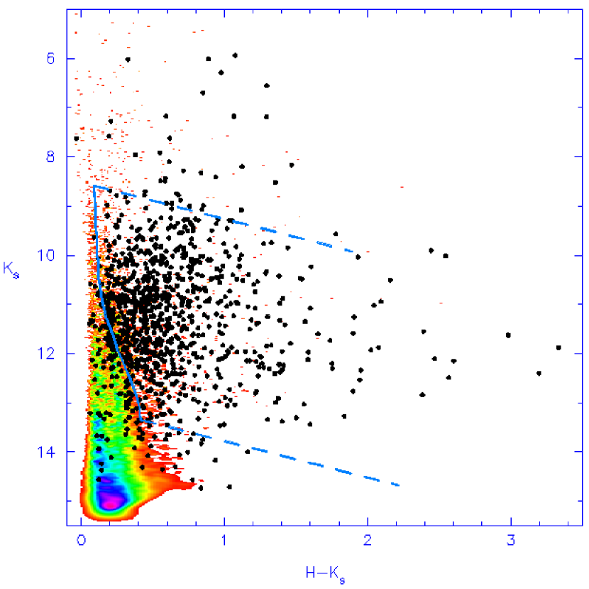
Figure 16: $K_{s}$ vs. $H-K_{s}$ color-magnitude diagram for all stars (color scale) and the variable stars (black circles) identified from the 16 nights in which all tiles were observed. For reference, the solid blue curve shows the 1 Myr pre-main-sequence isochrone from D’Antona & Mazzitelli (1997) for stellar masses between 0.08 M_⊙ and 3.0 M_⊙. The dashed lines indicate the reddening vector for 10 magnitudes of visual extinction from Cohen et al. (1981) transformed into the 2MASS photometric system (Carpenter, 2001). The lowest halftone is 1% of the peak density. This figure shows that the observed magnitudes and colors for the majority of the variable population is consistent with reddened pre-main-sequence stars with masses $\mathbin{\lower 3.0pt\hbox{$\hbox to0.0pt{\raise 5.0pt\hbox{$\char 60\relax$}\hss}\mathchar 29208\relax$}}$ 3 M_⊙.

The $K_{s}$ vs. $H-K_{s}$ color-magnitude diagram shown in Figure 16 further supports the conclusion that most of the variable stars are young ($\mathbin{\lower 3.0pt\hbox{$\hbox to0.0pt{\raise 5.0pt\hbox{$\char 60\relax$}\hss}\mathchar 29208\relax$}}$ 1 Myr), low mass ($\mathbin{\lower 3.0pt\hbox{$\hbox to0.0pt{\raise 5.0pt\hbox{$\char 60\relax$}\hss}\mathchar 29208\relax$}}$ 1 M_⊙), moderately reddened members of the Orion A molecular cloud. The color scale in this figure represents all detected stars, $\sim$ 85% of which are likely field stars (see the Appendix). The non-variable stars (predominantly field stars) are located primarily to the left of the 1 Myr isochrone, while most of the variable stars (filled symbols) are located to the right and are consistent with reddened pre-main-sequence objects.

To further examine the properties of the variable star population, Figure 17 shows the $J-H$ vs. $H-K_{s}$ color-color diagram for all stars in our sample (left panel) compared to the variable stellar population (right panel). This figure shows that the majority of non-variables have colors consistent with unreddened main sequence stars either in front of the cloud or at a variety of distances but along lines of site exterior to the cloud boundaries, or reddened main sequence and giant stars seen through the cloud. The variable stars are systematically redder compared to the non-variable stars, many with colors that place them in a region of the diagram that cannot be explained by interstellar extinction. These near-infrared colors are characteristic of young, low mass Classical T Tauri stars (CTTS’s) surrounded by optically thick accretion disks (Lada & Adams, 1992; Meyer, Calvet, & Hillenbrand, 1997) and moderately reddened. Approximately 30% of the variable stars have near-infrared colors consistent with CTTS’s as identified in the $J-H$ vs. $H-K_{s}$ color-color diagram, suggesting that up to 50% of the variable star population may be CTTS’s if the efficiency factor for this diagram as described in the Appendix of Hillenbrand et al. (1998) is adopted. Many of the variable stars, however, do not have such distinctive near-infrared colors. The variable stars without substantial near-infrared excesses are either CTTS’s with small excesses or weak-line T Tauri stars (WTTS’s) which as a class do not have strong signatures of optically thick circumstellar disks. Near-infrared variability therefore appears to be a characteristic of both CTTS’s and WTTS’s.

5 Characteristics of the Variability

After establishing that most of the near-infrared variable stars are young, low mass stars associated with the Orion A molecular cloud, we now investigate in more detail the variability characteristics exhibited by these stars. Our goal is to use the statistics inherent in our large sample to categorize the predominant types of near-infrared photometric fluctuations. To include as complete a sample as possible in characterizing the photometric variations, we incorporate all of the March/April 2000 time series data for the stars listed in Table 4 (unless otherwise stated). Strictly speaking, this results in non-uniform time coverage for stars as a function of their location in the survey region and also incorporates some stars that were included as variables based on somewhat subjective criteria. In practice, however, $\sim$ 77% of the variables are located in the center tiles 3-5 (see Table 2) and were observed on at least 25 of the possible 29 nights. Further, the number of stars included in the variable star list for reasons other than high Stetson index amount to less than 10% of the entire sample. Therefore, the following results should closely reflect those obtain from a more uniformly selected sample.

5.1 Amplitude of Magnitude and Color Changes

The amplitude of the variability was characterized by computing the observed RMS and peak-to-peak fluctuations in the magnitudes and the colors for individual stars. Since the observed photometric fluctuations reflect both actual astrophysical variability and photometric noise, a statistical correction needs to be applied to recover the intrinsic amplitude. For the RMS values, the actual variability amplitude ($\sigma_{\rm var}$) was estimated by subtracting in quadrature the expected RMS due to photometric noise ($\sigma_{\rm noise}$; see Eq. 3) from the observed RMS ($\sigma_{\rm obs}$; see Eq. 2) as

$$\sigma_{\rm var}=\sqrt{\sigma_{\rm obs}^{2}-\sigma_{\rm noise}^{2}}.$$ (6)

The noise correction for the peak-to-peak amplitudes is not as straight forward since it depends on the noise in the individual observations (which vary in the time series data) and the number of samples. A Monte Carlo simulation was run 500 times for each star to estimate the average expected peak-to-peak amplitude due to noise given the number of measurements and the photometric uncertainties. This expected peak-to-peak amplitude was subtracted linearly from the observed value to estimate the intrinsic peak-to-peak fluctuations.

Histograms of the peak-to-peak and RMS amplitudes for the magnitudes and colors, after correcting the observed values for the photometric noise, are shown in Figure 18 and Figure 19. The top panels in each figure show the histogram over the full dynamic range of the amplitudes, and the bottom panels emphasize the distribution at low amplitudes where most of the variable stars in fact reside. Statistics on the maximum, mean, median, and dispersion in the amplitudes are summarized in Table 6. The peak-to-peak fluctuations in the magnitudes are a couple tenths on average, but can be as large as 2.3^m at $J$-band and 1.2^m at $K_{s}$-band. Peak-to-peak fluctuations as large as 1.7^m at $K_{s}$-band are observed in three stars when the March 1998 are included. Fluctuations in the colors are less pronounced, as most of the photometric variations are essentially colorless within the photometric noise of the data. Thus stars that exhibit large magnitude and color variations (see, e.g., Figures 8-11) are among the more extreme cases of near-infrared variability in our sample.

5.2 Correlation of Magnitude and Color Changes

For stars with significant color variations, any correlation between the color-magnitude and color-color changes can serve as a clue to the origin of the variability. Cases of stars becoming bluer as they fade (e.g. Fig. 8) and others becoming redder as they fade (e.g. Fig. 9-11) exist in our data, with the photometric changes within a star usually well correlated along narrow vectors in the various color-color and color-magnitude diagrams. However, not all possible vector orientations are found in the time series data. To quantify the observed correlations, the slopes of the photometric variations in the $J$ vs. $J-H$, $K_{s}$ vs. $H-K_{s}$ and $J-H$ vs. $H-K_{s}$ diagrams were computed for individual stars. For each correlation, only stars in which the observed RMS in the colors exceeded the expected photometric uncertainties by 50% were included so that the derived slopes would not be dominated by noise in the data. As only $\sim$ 10% of the variable stars satisfied this criterion, the analysis that follows is most appropriate for those objects with relatively large-amplitude color variations and may not be applicable to those with largely colorless variability. The routine FITEXY (Press et al., 1992), which incorporates uncertainties in both axes in computing the best fit linear model to the data, was used to derive the slopes. A slope angle of 0° is defined as positive color change along the X-axis with no magnitude or color change along the Y-axis. The slope angle increases counter clockwise in the color-color diagram and clockwise in the color-magnitude diagram (since magnitudes are plotted with decreasing values towards the top).

Histograms of the derived slopes in various color-magnitude and color-color diagrams are shown in Figure 20. The open histogram represents all stars for which slopes were derived. The hatched histogram are stars where the slopes have been determined to better than 20% accuracy, with a typical 1$\sigma$ uncertainty of $\mathbin{\lower 3.0pt\hbox{$\hbox to0.0pt{\raise 5.0pt\hbox{$\char 60\relax$}\hss}\mathchar 29208\relax$}}$ 5°. In the $J-H$ vs. $H-K_{s}$ diagram, all but 5 of the stars have positive slopes between $\sim$ 30° and 60°. The photometric correlations for the 5 stars with negative slopes do not vary along a well-defined vector in the color-color diagram and the slope is not meaningful. Thus the dominant type of photometric variability in the near-infrared color-color diagram has both colors becoming redder together. In the $J$ vs. $J-H$ diagram, the predominant trend is that stars become fainter as the colors get redder with a slope between $\sim$ 50° and 80°. Two stars have negative slopes with uncertainties less than 20%; both are long term variables with large magnitude and color variations revealed by including the March 1998 data. In the $K_{s}$ vs. $H-K_{s}$ diagram the derived slopes show two distinct trends. In addition to stars with colors becoming redder as they fade (positive slopes; e.g. Figs. 9-11), a number of variables have colors becoming bluer as the stars become fainter (negative slopes; e.g. Fig. 8); $\sim$ 1% of the total number of variables are of this kind.

Figure 21 compares $J-H$ vs $H-K_{s}$ color-color diagrams for stars with positive and negative slope in the $K_{s}$ vs. $H-K_{s}$ color-magnitude diagram. (This figure also includes a panel for periodic stars, which are discussed in Section 5.3.2.) The majority ($\sim$ 90%) of variable stars do not have large color variations and do not appear in this figure. On average, the stars with large color variations tend to have redder near-infrared colors compared to the variable star population as a whole (see Fig. 17). Further, $\sim$ 76% of the stars with positive slope variations have near-infrared excesses characteristic of CTTS’s, compared to $\sim$ 53% of the small number of stars with negative slope variations and 30% for the uniformly select variable star population of $\sim$ 1000 stars (Section 4.3).

5.3 Temporal Properties

5.3.1 Time scales for Variability

The temporal variability characteristics can be evaluated on time periods of 1 day to $\sim$ 1 month using the March/April 2000 observations, on $\sim$ 2 month time scales by incorporating the February 2000 data, and on $\sim$ 2 year time scales with addition of the March 1998 data. The temporal properties of the March/April 2000 observations were evaluated using the autocorrelation function (ACF), which measures the similarity of photometric measurements over different time samples. While photometry is nominally available in our data set on a daily basis, the time series can contain gaps of up to 4 days. To account for this non-uniform sampling, the Fourier transform of the observed measurements was computed using the Scargle (1989) algorithm for unevenly sampled data. The power spectrum was then computed from the Fourier transform, and the inverse transform of the power spectra yielded the ACF. The resulting ACF was normalized by the ACF of the sampling function for each star (Scargle, 1989) and was sampled every 1 day in accordance with the nominal separation between our observations. A positive value of the ACF at a given time indicates that the photometry is correlated on that time scale, while negative value indicates the photometry is uncorrelated. The time scale of the variability can then be characterized by computing the largest time lag before the ACF first becomes negative. Since the mean value of the photometry was subtracted from the data before computing the ACF, the time lag is a crude measure of the number of consecutive days a star remains brighter or fainter than the mean magnitude over the time series. The longest variability time scale that can be estimated from the data then is approximately half of the total time period of the observations. The maximum time scale will vary between 9-18 days depending on the spatial location of the star. For variable stars locate in the center three tiles ($\sim$ 77% of the total number of variable stars), the maximum variability time scale that can be inferred is $\sim$ 14 days.

For random noise with an infinite number of samples, the distribution of time lags is a delta function at $\Delta t=0$; a finite number of samples though broadens the ACF. To estimate the expected distribution of time lags for random noise, the ACF was computed for each star as described above but replacing the observed magnitudes by a random number with a gaussian probability distribution with dispersion given by the photometric uncertainties. The time sampling in these simulated data are identical to that in the real observations.

Figure 22 shows the inferred time lags in the three bands for all identified variables (solid lines) and the simulated $J$-band data (dotted line). The $H$ and $K_{s}$ band simulated data are similar to the $J$-band simulation and for clarity are not shown. This figure demonstrates that the random noise data has a peak near zero time lag as expected since each data point is independent. By contrast, the distribution of time lags for the variable stars peaks at 1 day and has a more extended tail toward larger time lags than the simulated observations. The shape of these distributions suggests then that most of the variability occurs on time scales of less than a few days.

The near-infrared variability characteristics on $\sim$ 2 month and 2 year time scales were assessed using the February 2000 and March 1998. (Note that the February 2000 data are available only for sources north of $\delta=-6$°.) A long term variable was identified as a star in which the $J$, $H$, or $K_{s}$ magnitudes from these earlier measurements differed from the average March/April 2000 data by more than four times the observed RMS scatter in that time period. A 4$\sigma$ deviation was chosen since only $\sim$ 1 star in the entire source list should exhibit a fluctuation that large due to random noise. Given typical photometric uncertainties for the variable stars of 0.02-0.03^m, the 4$\sigma$ criteria imposes a minimum amplitude change of $\sim$ 0.1^m. By this definition, a total of 14 stars exhibited variability in the February 2000 data, but only 5 of these were variables not previously identified based on the Stetson index in Sample 1 or Sample 2 (see Table 3). A total of 72 stars exhibited significant photometric fluctuations on $\sim$ 2 year time scales, with 26 of these new variables not previously identified from the March/April 2000 data based on the Stetson statistic. The fact that few new long term variables were identified indicates that most of the short term variations are not part of larger amplitude variations occurring long time periods.

5.3.2 Periodic Behavior

The properties of variable stars can be further characterized by determining if the photometric variations are typically aperiodic or periodic. The Lomb periodogram algorithm in Press et al. (1992) was used to compute the power spectrum of all 17,808 stars in our sample and to determine the “false alarm probability” (FAP) that the highest peak in the power spectrum could result by chance. The highest frequency searched was 0.5 days^-1, and the shortest independent frequency was the reciprocal of the time period of the March/April 2000 data sequence for that star. So that at least 2 full cycles are present in the time series data, only periods less than half the total time span of the observations were considered reliable. Stars in the overlap regions of adjacent tiles have more than one photometric measurement recorded per night. Such clumping in the time sampling can invalidate the FAPs, and therefore only one of the overlap measurements was considered. The power spectrum and FAP were computed in this manner for all stars and in each band that contain $\geq$ 8 reliable photometric measurements.

Due to the multi-band nature of our time series data, the periodicity derived for a star can have high significance under several different scenarios. In generating a list of periodic stars we nominally required that the false-alarm-probability be $\leq 10^{-4}$ in any one of the following combinations: (1) a single band, (2) the product of any two bands, or (3) the product in all three bands. In practice, only one star had a FAP less than $10^{-4}$ in a single band. The effective single-band FAP through this procedure is $\sqrt{10^{-4}}\approx 0.01$ for two bands and $\root 3 \of{10^{-4}}\approx 0.05$ for three bands. When the product of the FAP in two or three bands was used, it was further required that the periods agree to within 20%.

Table 7 summarizes the periods and false-alarm-probabilities for the 233 stars identified as periodic variables in this study. Only 8 (3.4%) of these periodic sources were not identified as variable stars from the Stetson statistic. Conversely, the fraction of the near-infrared variable star population that is periodic is $\sim$ 18%, however, this is a lower limit to the actual percentage given the conservative FAP limits used to establish periodicity. If a FAP of 10^-3 is used, an additional $\sim$ 100 stars are identified with consistent periods in all three bands. Furthermore, optical monitoring studies have identified $\sim$ 760 periodic stars within a $\sim$ 60′ radius of the Trapezium region of the ONC (Stassun et al., 1998; Herbst et al., 2000; Rebull, 2001), only $\sim$ 100 of which are in common to our periodic stars. The $J-H$ vs. $H-K_{s}$ color-color diagram for the periodic stars identified in our sample is shown in Figure 21, where it is shown that most of the periodic stars have colors consistent with WTTS’s.

To verify that our criteria produced a reliable sample of periodic stars, robust estimation with replacement (Press et al., 1992) was used to find the number of false periods one would expect to detect among the 17,808 stars in our sample. For each time sample, the observed magnitude was replaced by a magnitude chosen randomly from the time series photometry for that star. The $J$, $H$, and $K_{s}$ photometry were re-distributed in parallel since the coincidence of periodic behavior in these bands were used to select periodic stars from the real data. The power spectra of the redistributed data were computed and the number of significant periodic stars assessed using the same criteria described above. Of the 17,808 stars in the Monte Carlo simulation, only 2 were identified as periodic.

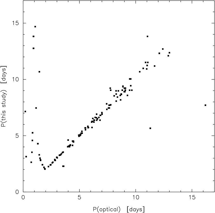
Figure 23: Comparison of the optical, $I$-band periods (Stassun et al., 1998; Herbst et al., 2000; Rebull, 2001) with the $H$-band periods derived in this study. For $\sim$ 80% of the stars, the optical and near-infrared periods agree to better than 10%. Stars with periods less than $\sim$ 2 days as indicated by the optical data are aliased to longer periods in this study due to the 1 day time sampling of the near-infrared observations. Stars that have optical periods roughly twice that of the near-infrared period may be examples of “period doubling” which results when multiple star spots are present (Herbst et al., 2000). One star with an optical period of $\sim$ 60 days and a near-infrared period of $\sim$ 14 days is not shown in this figure since the optical period is uncertain (Rebull, 2001).

Finally, we examined the accuracy of our derived periods by comparing them with those found from optical monitoring observations (Stassun et al. 1998; Herbst et al. 2000; Rebull 2001 and references therein). Figure 23 compares the periods for 109 stars identified as periodic at both optical ($I_{C}$) and near-infrared ($J$ and/or $H$ and/or $K_{s}$) wavelengths. The periods agree to within 10% for $\sim$ 80% of the stars, suggesting that for these stars the origin of the periodicity is the same at optical and near-infrared wavelengths. The biggest discrepancy in the derived periods occurs when our reported period is actually an alias of a more significant period at $<$2 days found from optical monitoring at higher time resolution than our time series. Figure 23 suggests that this occurs for $\sim$ 10% of the stars in our periodic sample. Three of the stars with optical periods greater than 10 days have near-infrared periods that differ by a factor of two or more. In a few cases, the near-infrared period is approximately half that of the optical period. These may be examples of “period doubling”, where the presence of two star spots on opposite sides of the star causes the periodogram analysis to derive a period half that of the actual value (Herbst et al., 2000). The other discrepant source (with an optical period of $\sim$ 60 days and a near-infrared period of $\sim$ 14 days) has been noted to have uncertain optical period (Rebull, 2001).

A histogram of our derived periods is shown in Figure 24. The shaded region indicates periods that are suspected aliases of sub-2 day periods based on comparison with optical monitoring data; only $\sim$ 1/2 of our periodic sample has the information necessary to make this comparison due largely to our larger spatial coverage compared to optical period searches. The frequency distribution is characterized by a peak at 2-3 days and a slow decline towards longer periods. The range of amplitudes and periods to which our data are sensitive was established by replacing the time series data for each variable star with a sinusoidal signal plus gaussian random noise that has a dispersion equal to the photometric noise of the actual data. Periodic stars in these simulated data were then identified as described above using an maximum effective FAP of 10^-4. The results indicate that our data are roughly uniformly sensitive to periods between 2 and 10 days, although with reduced sensitivity at 2 and 3 days due to the 1 day time sampling of the observations. Approximately half of the simulated stars with peak-to-peak amplitudes of $\sim$ 0.08^m and $\sim$ 90% with peak-to-peak amplitudes of 0.16^m were identified as periodic in the simulations. By comparison, 55% of the total variable star population and 60% of the identified periodic stars have $H$-band peak-to-peak amplitudes $\geq 0.08$^m.

6 Origins of Near-Infrared Variability

We turn now from observational characterization of the near-infrared photometric variations to examination of possible physical origins of the variability. The primary observational constraints as established in Section 5 are (1) nearly all of the identified variables are young, low mass stars associated with the Orion A molecular cloud; (2) the typical time scale for the variability is a few days or less; (3) the light curves exhibit a variety of features ranging from periodic behavior, to discrete variability episodes superposed on otherwise steady light curves, to smooth photometric variations over several days, to month long (or longer) rises and fades; (4) the amplitudes of the fluctuations are $\sim$ 0.2^m on average, but can reach $\sim$ 2^m in the extreme; and (5) the photometric fluctuations are nearly colorless in most cases, with $\sim$ 77% of the variable stars having color variations $<$0.05^m.

Both the spatial distribution and the observed colors and magnitudes of the variable stars are consistent with what is expected for the Orion pre-main-sequence population, suggesting that much of the observed near-infrared variability is intimately related to the properties of young stellar objects. Further, the short time scale for the photometric fluctuations suggests that the variability originates either within the stellar photosphere or close to it in the inner circumstellar environment. As established by previous studies (Rydgren & Vrba, 1983; Liseau, Lorenzetti, & Molinari, 1992; Kenyon et al., 1994; Skrutskie et al., 1996; Hodapp, 1999), there are several short term phenomena related to young stellar objects that may contribute to near-infrared variability, including rotational modulation by cool and hot spots on the stellar surface, changes in the line-of-sight obscuration due to circumstellar dust, variations in accretion geometry or mass transfer rates from circumstellar disks, and gradual declines in brightness from EX Lup or FU Ori type bursts. Mechanisms not necessarily unique to young stellar objects may also be operative, such as eclipses due to binary companions. Many of these mechanisms were first suspected from optical monitoring observations of young stellar objects (e.g. Herbst et al. 1994; Bouvier et al. 1999). Infrared observations, however, uniquely probe variability related to circumstellar material which radiates at temperatures too cold ($\mathbin{\lower 3.0pt\hbox{$\hbox to0.0pt{\raise 5.0pt\hbox{$\char 60\relax$}\hss}\mathchar 29208\relax$}}$ 2000 K) to contribute substantially to optical emission.

In the following sections we investigate the amplitudes and the time scales expected for photometric fluctuations due to star spots, extinction, and accretion disk phenomena. We begin by analyzing the contributions from cool and hot spots since these are known to exist on young stars from optical studies and must contribute to near-infrared variability as well. However, as will be shown, star spots cannot explain all of the observed near-infrared variability characteristics and other mechanisms must be present, with extinction and accretion-related phenomenon as strong candidates. While throughout this discussion we consider the effects of these mechanisms separately, in reality, a number of mechanisms may be operating simultaneously for any individual star.

6.1 Star Spots

6.1.1 Models

Star spots, which can be either cooler or hotter than the photospheric temperature, modulate the brightness of a star as stellar rotation alters the fractional spot coverage visible to the observer. Cool spots are thought to arise from magnetic activity on the stellar surface, whereas hot spots are interpreted as regions where material accreting along magnetic field lines (e.g. Hartmann, Hewett, & Calvet 1994) impacts the star. Instead of discrete hot spots, a more realistic model may be one in which the accretion is confined to a high latitude ring on the stellar surface, where the inclination of the ring with respect to the stellar rotation axis depends on the orientation of the dipole magnetic field (see, e.g., Mahdavi & Kenyon 1998). In this scenario, variability may result either from simple rotation of the inclined accretion ring around the star, or from non-steady accretion.

The photometric amplitudes expected from both cool and hot star spots were calculated assuming that spots can be characterized by a single temperature blackbody, $T_{\rm spot}$, that covers a fraction, $f$, of the stellar photosphere with an effective temperature $T_{*}$. The amplitude of the photometric variations, relative to pure photospheric emission, can then be expressed as (see, e.g., Vrba et al. 1986)

$$\Delta m(\lambda)=-2.5\>{\rm log}_{10}\{1-f[1.0-B_{\lambda}(T_{\rm spot})/B_{\lambda}(T_{*})]\},$$ (7)

where $B_{\lambda}(T)$ is the Planck function. This star spot model ignores limb darkening, inclination effects, and opacity differences as a function of wavelength between the spot and the stellar photosphere. The models shown in Figure 25 assume a stellar effective temperature of 4000 K, corresponding to a 0.5 M_⊙ star at age 1 Myr (D’Antona & Mazzitelli, 1997), and cool and hot spot temperatures of 2000 K and 8000 K respectively. Results are presented for spots that cover 1, 2, 5, 10%, 20%, and 30% of the stellar surface. These models encompass the more extreme spot parameters inferred from optically selected sample of low mass pre-main-sequence stars (Bouvier & Bertout, 1989; Bouvier et al., 1993; Fernández & Eiroa, 1996).

Figure 25 shows that cool and hot spots can be distinguished observationally in the near-infrared based on the amplitude of the photometric fluctuations. While hot and cool spots with small fractional coverages both produce low amplitude, nearly colorless fluctuations, the maximum amplitude from cool spots is $\sim$ 0.4^m at $J$-band, while hot spots can produce photometric fluctuations as large as 1^m for sufficiently hot spot temperatures and/or large fractional coverages. Further, the maximum changes in the $J-H$ and $H-K_{s}$ colors that can be produced with the spot parameters considered here is $\sim$ 0.03^m for cool spots but 0.1-0.2^m for hot spots.

The time scale for variability caused by cool or hot star spot modulation is governed by the stellar rotation period. The frequency distribution of periods in T Tauri stars derived from optical monitoring observations imply rotation periods of $\mathbin{\lower 3.0pt\hbox{$\hbox to0.0pt{\raise 5.0pt\hbox{$\char 60\relax$}\hss}\mathchar 29208\relax$}}$ 10 days for $\sim$ 90% of the known periodic stars in Orion (Stassun et al., 1998; Herbst et al., 2000; Rebull, 2001), assuming that the observed periodicity is a result of rotational modulation by star spots. Similar rotation periods have been derived from Doppler imaging of T Tauri stars (Joncour, Bertout, & Bouvier, 1994; Rice & Strassmeier, 1996; Johns-Krull & Hatzes, 1997; Neuhäuser et al., 1998). Rotational velocities derived from high resolution spectroscopy ($v\ {\rm sin}\>i$) also imply that young stellar objects have rotational periods on the order of a few days (Bouvier et al., 1986; Hartmann et al., 1986). Time scales of a few days are consistent with the results of our ACF analysis (Section 5.3.1).

Cool and hot spots are perhaps distinguishable based not on the time scale of the photometric variability, but on the time scale over which it persists. Cool spots are thought to be relatively stable features that can last several years or more. Hence observed periodicity is often a repeatable result, especially in WTTS’s which do not have additional variability components related to accretion phenomena. Hot spots, however, generally last only a few days or weeks as evidenced by period changes and even disappearance/reappearance in a few cases where hot spot periods have been detected (Vrba et al. 1989,1993). Thus hot spots tend to produce irregular variability, especially if the accretion of material onto the star is unsteady as has been inferred in some stars (Gullbring et al., 1996; Basri, Johns-Krull, & Mathieu, 1997; Smith et al., 1999), or if the geometry is complicated by misaligned rotation and magnetic dipole axes (e.g. Mahdavi & Kenyon 1998; Bouvier et al. 1999). Based on these tendencies, Herbst et al. (1994) introduced a classification scheme in which periodic fluctuations from cool spots (mainly in WTTS’s, but in some CTTS’s as well) are Type I variables, irregular fluctuations in CTTS’s from hot spots are Type II variables, and periodic fluctuations in CTTS’s from hot spots are Type IIp variables. (Type III variability in this classification scheme is discussed in Section 6.3).

6.1.2 Comparison to Observations: Cool Spots

For cool spot parameters typically inferred from optical observations ($T_{*}$-$T_{\rm spot}$ $\mathbin{\lower 3.0pt\hbox{$\hbox to0.0pt{\raise 5.0pt\hbox{$\char 60\relax$}\hss}\mathchar 29208\relax$}}$ 2000 K, $f$ $\mathbin{\lower 3.0pt\hbox{$\hbox to0.0pt{\raise 5.0pt\hbox{$\char 60\relax$}\hss}\mathchar 29208\relax$}}$ 30%; see Bouvier & Bertout 1989, Bouvier et al. 1993, Fernández & Eiroa 1996), the expected peak-to-peak amplitudes should be $\mathbin{\lower 3.0pt\hbox{$\hbox to0.0pt{\raise 5.0pt\hbox{$\char 60\relax$}\hss}\mathchar 29208\relax$}}$ 0.4^m in the $J$, $H$, and $K_{s}$ bands and $\mathbin{\lower 3.0pt\hbox{$\hbox to0.0pt{\raise 5.0pt\hbox{$\char 60\relax$}\hss}\mathchar 29208\relax$}}$ 0.03^m in the $J-H$ and $H-K_{s}$ colors (Figure 25). These amplitudes are only approximate given the simplicity of the model with the essential predictions that the color variations from cool spots should be relatively low and appear periodic (moreso in WTTS’s than CTTS’s) by analogy with Type I optical variability (Herbst et al., 1994, see also Herbst, Maley, & Williams 2000). In our data, 65% of the periodic variables stars have amplitudes $\leq$ 0.4^m at $J$-band and $\leq$ 0.03^m in the $J-H$ color, 77% have color amplitudes $\leq$ 0.05^m, and 80% have near-infrared colors consistent with WTTS’s. Thus rotational modulation by cool spots can account for the variability characteristics in the majority of the periodic stars.

Periodic stars, however, account for only $\sim$ 18% of the total variable population, and an additional $\sim$ 600 stars ($\sim$ 50% of the identified variables) also have low amplitude, nearly colorless photometric fluctuations but have not been identified as periodic. While arbitrarily low photometric fluctuations can be produced by many of the physical mechanisms discussed in this section, Figure 26 suggests that rotational modulation by cool spots may cause much of the low amplitude variability, independent of whether a period is actually detected. This figure shows the $J-H$ vs. $H-K_{s}$ color-color diagram as a function of the peak-to-peak $J$-band amplitude. Most stars with low amplitudes ($\leq$ 0.2^m) have near-infrared colors consistent with WTTS’s or stars with small infrared excesses. As the $J$-band amplitude increases, the near-infrared colors tend to become redder and an increasing fraction contain a near-infrared excess characteristic of the optically thick circumstellar disks of CTTS’s. This trend suggests that different mechanisms related to the absence or presence of an accretion disk may be producing the low and high amplitude variability. Of the variability mechanisms examined here, only cool spots and eclipsing binaries do not require the presence of a circumstellar disk. Since eclipsing systems cannot account for the large number of stars with low amplitude variability, cool spots appear as a more likely explanation.

Cool spot modulation produces larger amplitude fluctuations at optical wavelengths, and so optical surveys should provide a more complete census of the periodic variables. As mentioned in Section 5.3.2, optical studies have found $\sim$ 750 periodic stars in the Orion Nebula region (Stassun et al., 1998; Herbst et al., 2000; Rebull, 2001), of which $\sim$ 330 are identified as near-infrared variables and $\sim$ 100 as periodic in this study. Of those optical periodic stars also identified as near-infrared variables (but not necessarily periodic near-infrared variables), $\sim$ 70% have low peak-to-peak amplitudes in the $J$-band magnitudes ($\leq$ 0.4^m) and $J-H$ colors ($\leq$ 0.03^m). Further, $\sim$ 88% of the $\sim$ 650 optical periodic variables not identified as periodic in the near-infrared have near-infrared colors consistent with reddened WTTS’s.

Based on the observational evidence just described we speculate that the photometric fluctuations observed in many of the low amplitude variable stars are due to cool spot modulation. As a lower limit to the star that may have variability due to cool spot modulation, we find that 57% of the variables have $J$-band amplitudes $\leq$ 0.4^m, $J-H$ amplitudes $\leq$ 0.03^m, and no near-infrared excess as expected for cool spot parameters inferred from optical observations. Given the simplicity of the star spot model, if we crudely assume that the maximum $J-H$ color change that can be produced by cool spots is 0.05^m, we derive a upper limit of 77% as the percentage of the variability that may be attributed to cool spots.

6.1.3 Comparison to Observations: Hot Spots

While cool spots can plausibly account for the low amplitude variables with small color variations, they cannot explain the 23% of the variable stars that have color variation exceeding $\sim$ 0.05^m (see Fig. 25). Stars with significant color variations were analyzed in Section 5.2 where it was shown that these objects tend to have colors consistent with CTTS’s (see Fig. 20). Therefore, again by analogy with optical variability characteristics, we investigate whether hot spots, which cause Type II optical variability in CTTS’s in the Herbst et al. (1994) classification scheme, can account for the color amplitudes observed in some of the near-infrared variable stars.

For hot spot parameters typically inferred from optical observations ($T_{\rm spot}$ $\mathbin{\lower 3.0pt\hbox{$\hbox to0.0pt{\raise 5.0pt\hbox{$\char 60\relax$}\hss}\mathchar 29208\relax$}}$ 8000 K, $f$ $\mathbin{\lower 3.0pt\hbox{$\hbox to0.0pt{\raise 5.0pt\hbox{$\char 60\relax$}\hss}\mathchar 29208\relax$}}$ 10%), hot spots can cause peak-to-peak amplitudes at near-infrared wavelengths as large as $\sim$ 0.2-0.4^m in the magnitudes and $\mathbin{\lower 3.0pt\hbox{$\hbox to0.0pt{\raise 5.0pt\hbox{$\char 60\relax$}\hss}\mathchar 29208\relax$}}$ 0.06-0.12^m in the colors (see Fig. 25). About 10% of the near-infrared variable stars have magnitude and color amplitudes larger than these hot-spot predictions (see Section 5.2). A combination of hotter spot temperatures ($\mathbin{\lower 3.0pt\hbox{$\hbox to0.0pt{\raise 5.0pt\hbox{$\char 62\relax$}\hss}\mathchar 29208\relax$}}$ 10,000 K) and higher coverages ($\mathbin{\lower 3.0pt\hbox{$\hbox to0.0pt{\raise 5.0pt\hbox{$\char 62\relax$}\hss}\mathchar 29208\relax$}}$ 20%) are needed to explain these stars from hot spots alone. These spots parameters are evidently rare, but may be possible and simply not identified previously due to small number statistics that are overcome by the extensive near-infrared variable sample obtained here.

Because of the substantial color variability expected from hot spots, a more quantitative comparison between the observations and the hot spot model can be made by assessing correlated color and magnitude changes in individual stars. Figure 20 showed the observed slopes in various color-color and color-magnitude diagrams as discussed in Section 5.2. The predicted slope from the hot spot model is also indicated on this figure, which varies only by a few degrees for stellar effective temperatures between 3000 and 6000 K and spot temperatures up to 40,000 K. Figure 20 shows that many of the observed slopes in the $J$ vs. $J-H$ diagram can be accounted for quantitatively by hot spots (and extinction variations as discussed in the following section). However, in the $J-H$ vs. $H-K_{s}$ and $K_{s}$ vs. $H-K_{s}$ diagrams, while there is an approximate correspondence between the observed and predicted slopes, the observed slopes are systematically shallower than expected if the variability is due solely to hot spots. These differences may not be significant though given the simplicity of the hot spot model. In addition, the $K_{s}$ vs. $H-K_{s}$ diagram contains a number of stars with negative slopes in that the colors become bluer as the star gets fainter. Such variations are completely inconsistent with the hot spot model, and suggest that additional mechanism(s) are present that contribute to the near-infrared variability, especially at $K_{s}$-band.

6.2 Extinction

6.2.1 Models

Variability due to extinction can result from inhomogeneities in either the inner circumstellar environment or the ambient molecular cloud that move across the line of site. Photometric changes induced by visual extinction variations of $\Delta{\rm A_{V}}=\pm 2$^m are illustrated in the middle column in Figure 25, although the extinction changes in practice can be of arbitrary value. The extinction vectors were calculated from the interstellar reddening law measured by Cohen et al. (1981) and transformed into the 2MASS photometric system (Carpenter, 2001). If the extinction variations originate from a circumstellar disk and the dust grains have conglomerated into larger particles to produce a more grey extinction law, the amplitude of the color variations will be less than indicated. For the interstellar reddening law, Figure 25 shows that extinction variations produce photometric slopes at near-infrared wavelengths similar to those expected from hot spots except in the $K_{s}$ vs. $H-K_{s}$ diagram, where the extinction slope is shallower by $\sim$ 25°.

The time scale for extinction variations caused by the ambient molecular cloud is set by the size scale of the structural inhomogeneities and the velocity field of the molecular gas. The typical line of sight full-width-at-maximum line width observed in the Orion molecular cloud from single dish ¹³CO(1–0) observations is $\sim$ 2 km s^-1 (Bally et al., 1987). Thus the time scale for one point in the cloud to transit a 1.5 R_⊙ radius star (representative of a $\sim$ 0.5 M_⊙ at an age of 1 Myr) is $\sim$ 12 days. The line wings in molecular line profiles can extend to several kilometers per second, which may shorten the appropriate time scales to a few days.

If structural inhomogeneities in a circumstellar disk occult the star to cause extinction variations, a variety of time scales are possible. Possible inhomogeneities include azimuthal asymmetries in the plane of the disk, a warped or flared outer disk (Bertout, 2000), or a warped/precessing inner disk (Lai, 1999; Bouvier et al., 1999; Terquem & Papaloizou, 2000). Azimuthal asymmetries or warped features will produce variability on time scales dictated by the rotational velocity of the disk and the size scales of the inhomogeneous features. The time for one position in the disk to transit the star ranges from hours within a few stellar radii to a week or more for radii $\mathbin{\lower 3.0pt\hbox{$\hbox to0.0pt{\raise 5.0pt\hbox{$\char 62\relax$}\hss}\mathchar 29208\relax$}}$ 30 AU. (If a warp extends for a significant azimuthal distance around the star, however, the relevant time scale will be given by the rotation period at that radius.) The fraction of the stars that show extinction variability will depend on the probability that these inhomogeneous features transit the star. These predictions are heavily model dependent, but Bertout (2000) suggests that as many as 20% of the stars with circumstellar disks may be occulted by the flared outer disk. Azimuthal asymmetries require viewing the disk nearly edge on, and are not likely to contribute substantially to the total number of variables. The magnetospheric accretion columns and the inner disk wind are likely optically thin and would not contribute to extinction variations (Kenyon, Yi, & Hartmann 1994 and references therein).

6.2.2 Comparison to Observations

If the ambient molecular cloud produces extinction variations, then the variable star population exhibiting significant color variations should contain a mixture of all (non-foreground) populations to which our survey is sensitive. This would include background field stars and Orion population stars with and without near-infrared excesses (i.e. CTTS’s and WTTS’s). Since field stars and WTTS’s outnumber CTTS’s, CTTS’s should be the least represented group in the variable star population. However, as shown in the left panel of Figure 21, stars with large color variations preferentially have near-infrared excesses characteristic of circumstellar disks and CTTS’s. This, combined with the longer time scale ($\sim$ 12 days) expected for cloud transit events compared to the typical observed variability time scale ($\mathbin{\lower 3.0pt\hbox{$\hbox to0.0pt{\raise 5.0pt\hbox{$\char 60\relax$}\hss}\mathchar 29208\relax$}}$ 3 days; see Figure 22) suggests that if extinction changes do contribute to near-infrared variability, the source of the extinction is in the inner circumstellar environment and not the ambient cloud.

Visual extinction variations of $\sim$ 10^m are need to account for the extreme magnitude and color variations indicated in Table 6. The typical observed variability time scale of $\mathbin{\lower 3.0pt\hbox{$\hbox to0.0pt{\raise 5.0pt\hbox{$\char 60\relax$}\hss}\mathchar 29208\relax$}}$ 3 days indicates that any inhomogeneities in the disk structure must transit the star within a similar interval. For a stellar radius of 1.5 R_⊙, the implied velocity of the inhomogeneous region is $\mathbin{\lower 3.0pt\hbox{$\hbox to0.0pt{\raise 5.0pt\hbox{$\char 62\relax$}\hss}\mathchar 29208\relax$}}$ 10 km s^-1. Assuming Keplerian rotation, the maximum radial distance from a 0.5 M_⊙ star that produces such velocities is $\sim$ 7 AU. If the size of the warp is significantly larger the stellar diameter, the warp would need to be located at smaller radial distances to be consistent with the observed variability size scale. This suggests that the outer disk flares described by Bertout (2000) are not likely responsible for the short term photometric variability observed here, but may still be contribute to the longer term fluctuations.

The slope of the photometric correlations shown in Figure 20 can also be used to test if the observed variability may be due to extinction variations. The expected slope of the interstellar extinction law is indicated by the filled squares in Figure 20. This figure shows that extinction variations (along with hot spots) can quantitatively explain most of the observed slopes in the $J$ vs. $J-H$ diagram. However, as with the hot spot model, extinction cannot in detail account for the observed slopes in the $J-H$ vs. $H-K_{s}$ and $K_{s}$ vs. $H-K_{s}$ diagrams. In the color-color diagram, the observed slopes are not as steep as expected from extinction. In the $K_{s}$ vs. $H-K_{s}$ diagram, while extinction can account for many of the observed slopes, the average observed slope is steeper than expected for interstellar extinction and shallower than predicted by hot spots. Invoking a more grey extinction (although not completely grey, as color variability is observed) would provide better agreement with the observed slopes in the $J-H$ vs. $H-K_{s}$ and $K_{s}$ vs. $H-K_{s}$ diagrams, but then could not simultaneously account for the already good agreement with the $J$ vs. $J-H$ slopes. Therefore, extinction cannot simply account for the observed variability characteristics. Further, similar to hot spots, extinction cannot explain any of the stars that have negative slopes in the $K_{s}$ vs. $H-K_{s}$ diagram.

6.3 Accretion Disks

The above discussion indicates that the simple star spot and extinction models cannot explain all of the variability characteristics of stars that exhibit color variations. The two main discrepancies are the slopes of the positive photometric correlations in the $J-H$ vs. $H-K_{s}$ and $K_{s}$ vs. $H-K_{s}$ diagrams (but not the $J$ vs. $J-H$ diagram), and any of the stars with negative slopes in the $K_{s}$ vs. $H-K_{s}$ diagram. This result suggests that an additional mechanism may be present that affects the emission at longer wavelengths more so than at shorter wavelengths. Since the stars that cannot be explained by the star spot and extinction models tend to have near-infrared excesses, we consider emission from a circumstellar disk as a source of near-infrared variability.

6.3.1 Models

Disks contribute to the near-infrared emission through two means. First, they absorb radiation from the star and re-radiate it at longer wavelengths, producing the infrared excess that is commonly observed in young stellar objects. The shortest wavelength at which a near-infrared excess is produced depends on how close the disk extends to the stellar surface and how hot the inner disk material becomes (Meyer, Calvet, & Hillenbrand, 1997). A second source of near-infrared emission from circumstellar disks occurs when energy is released as material is radially transported through a viscous, optically thick, accretion disk (Lynden-Bell & Pringle, 1974). Photometric variability due to a circumstellar disk can result then from changes in the mass accretion rate and consequently the accretion luminosity, or changes in the inner disk structure that alters the amount of absorbed and re-processed stellar radiation. Changes in the re-processed radiation may result, for example, from physical variations in the disk inner hole radius, or variations in the thickness of the inner edge of a warped disk. Such complicated inner disk geometries are predicted to occur when the dipole magnetic field is misaligned with the stellar rotation axis (Mayhavi & Kenyon, 1998; Lai, 1999; Terquem & Papaloizou, 2000).

Figure 25 shows the expected photometric variations for changes in the mass accretion rate and inner hole radius of a circumstellar disk around a star with an effective temperature of 4000 K. These model results are from the same models used by Meyer, Calvet, & Hillenbrand (1997), and were kindly provided by N. Calvet. The open and filled triangles in Figure 25 represent mass accretion rates of $M{\raise 6.45831pt\hbox{\hskip-6.0pt$\mathchar 513\relax$}\kern 1.99997pt}_{acc}$ = 10^-8.5 and 10^-7.0 M_⊙ year^-1, respectively, and for each accretion rate, the triangles represent the photometric emission for an inner hole radius of 1, 2, and 4 R_⊙, all for a disk inclination angle of 45°. As the inner hole radius increases, the star/disk system gets fainter in the near-infrared with less emission absorbed and reprocessed by the circumstellar disk. However, unlike the hot spot and extinction models, the system colors become bluer (approaching the stellar color) as it becomes fainter since the disk radiates more strongly at $K_{s}$-band than at $J$ or $H$. For hole sizes $\mathbin{\lower 3.0pt\hbox{$\hbox to0.0pt{\raise 5.0pt\hbox{$\char 62\relax$}\hss}\mathchar 29208\relax$}}$ 4  R_⊙ and a mass accretion rate of $\sim$ 10^-8.5 M_⊙ year^-1, no near-infrared excess emission is produced. The photometric variations expected from these disks models can be as large as 1^m at $K$-band for the hole sizes and accretion rates illustrated in Figure 25. Photometric variations of several magnitudes can be achieved if the accretion rates increase to $M{\raise 6.45831pt\hbox{\hskip-6.0pt$\mathchar 513\relax$}\kern 1.99997pt}_{acc}$ $\sim$ $10^{-5}$-$10^{-4}$ M_⊙ year^-1. These accretion disk models also predict a shallower slope in the $J-H$ vs. $H-K_{s}$ diagram than expected from extinction or hot spot variability, which is consistent with the observed locus of CTTS’s in this color-color diagram (Meyer, Calvet, & Hillenbrand, 1997).

To examine the time scales associated with viscous accretion disks, we considered an accretion disk around a 0.5 M_⊙ star using the $\alpha$ viscosity parameterization (Shakura & Sunyaev, 1973) and assuming $\alpha=0.01$ (Hartmann et al., 1998). The accretion rate can change globally within the disk or in a localized region. The time scale to transport material from the outer to the inner disk is $\mathbin{\lower 3.0pt\hbox{$\hbox to0.0pt{\raise 5.0pt\hbox{$\char 62\relax$}\hss}\mathchar 29208\relax$}}$ 1000 years for $M{\raise 6.45831pt\hbox{\hskip-6.0pt$\mathchar 513\relax$}\kern 1.99997pt}_{acc}$ $\sim$ 10^-8 M_⊙ year^-1 and radii greater than 1 AU (Frank, King, & Raine, 1985). Accretion rates may also vary if the disk equilibrium is perturbed. Thermal instabilities in the disk can be on the order of $\sim$ 1 day in the inner disk region given the uncertainty in $\alpha$ (Frank, King, & Raine, 1985). Another possible mechanism that may lead to variable mass accretion rates in the inner disk is a time-variable magnetic field. In the current paradigm of magnetospheric accretion, the size of the inner hole of a circumstellar disk in steady state is a function of the mass accretion rate and the stellar magnetic field strength (Königl, 1991). If the magnetic field strength varies in time, the magnetosphere will intersect the disk at a radius other than the corotation radius, which will modulate the accretion flow in the inner disk. Armitage (1995) and Clarke et al. (1995) (see also Kenyon, Yi, & Hartmann 1996) invoked this model to explain the variability characteristics in T Tauri stars over many years, but since the viscous time scale in the inner disk approaches $\sim$ 10 days for large values of $\alpha$, this may contribute to shorter term variability as well. Finally, the growth time of a warping instability in the inner disk, which may lead to variations in the amount of re-processed emission, is $\sim$ 6 days (Lai, 1999).

6.3.2 Comparison to Observations

The observed time scales of the near-infrared fluctuations rule out any global changes in the disk mass accretion rate (expected on time scales $\mathbin{\lower 3.0pt\hbox{$\hbox to0.0pt{\raise 5.0pt\hbox{$\char 62\relax$}\hss}\mathchar 29208\relax$}}$ $10^{3}$ years, if indeed occurring) as the origin of the near-infrared variability observed here. Short term variations in the mass accretion rate or geometry in the inner disk are somewhat speculative and it is not clear that they can in fact produce variability on time scales of days. Nonetheless, the following discussion considers short term variations in the disk properties as possible origins of the observed near-infrared photometric fluctuations.

The accretion disk models plotted in Figure 25 reproduce the observed locus of CTTS’s in the $J-H$ vs. $H-K_{s}$ color-color diagram (Meyer, Calvet, & Hillenbrand, 1997), and this observed CTTS’s locus slope is indicated in Figure 20. In the $J-H$ vs. $H-K_{s}$ diagram, the variable stars follow an observed slope that is steeper on average than expected from a time-variable disk (although extinction and hot spots are no more successful in uniquely explaining the observed slopes). In the color-magnitude diagrams, the observed slopes are positive, while the predicted slopes from the disk models are distinctly negative. Thus the majority of the stars exhibiting color variability can not have their variability explained solely by these disk models. However, a small number of stars ($\sim$ 17) do have negative observed slopes in the $K_{s}$ vs. $H-K_{s}$ diagram (see, e.g., Fig. 8) that agree quantitatively with that expected from the disk models. In fact, 7 of the 17 stars with significant negative slopes may have a near-infrared excess indicative of a circumstellar disk. About half of the stars with negative slopes do not show a near-infrared excess, although it should be noted that not all stars with $K_{s}$ excesses will be identified in the $J-H$ vs. $H-K_{s}$ diagram.

Finally, we briefly discuss the limits set by our data on the frequency of FU Ori type bursts in which a star brightens by several magnitudes in $\mathbin{\lower 3.0pt\hbox{$\hbox to0.0pt{\raise 5.0pt\hbox{$\char 60\relax$}\hss}\mathchar 29208\relax$}}$ 1 year, presumably due to a dramatic increase in accretion driven by large-scale disk instabilities (Hartmann, Kenyon, & Hartigan, 1993). All stars brighter than $K_{s}$=14^m in the March/April 2000 data are apparent in the March 1998 images, and the largest observed change in the $K_{s}$-band magnitudes is 1.7^m, with an approximately equal number of stars decreasing in brightness by $>$1^m as increasing over this $\sim$ 2 year period. Thus no convincing evidence exists for a FU Ori type burst in these monitoring observations. A lower limit on the time scale for such bursts is given then by the number of stars in the Orion A molecular cloud ($\sim$ 2700; see Appendix) and the time spanned by the observations ($\sim$ 2 years), or $\mathbin{\lower 3.0pt\hbox{$\hbox to0.0pt{\raise 5.0pt\hbox{$\char 62\relax$}\hss}\mathchar 29208\relax$}}$ 5400 years. This is consistent with the time scale between FU Ori bursts commonly assumed ($\sim$ 10⁴ years; Herbig 1977, Hartmann, Kenyon, & Hartigan 1993).

6.4 Eclipsing Systems

Although the above mechanisms are the leading candidates to account for most of the observed near-infrared variability, a small number of systems have variability properties consistent with eclipsing binary systems. This type of variability is distinguished by simultaneous drops in the $J$, $H$, and $K_{s}$ amplitudes on a single observation for the 1 day time interval of our observations (see, e.g., BM Ori in Fig. 6). As an initial screening for potential eclipsing systems, the March/April 2000 data was searched for stars in which at least 2 of the 3 bands decreased in brightness by more than 5$\sigma$ from the mean magnitude, where $\sigma$ is the observed photometric rms after excluding the faintest 20% of the measurements (as to exclude the actual eclipses from the RMS measurements). These criteria yielded 73 stars, all of which were previously identified as variable based on the Stetson index or other criteria. The light curves for these stars were then visually inspected to identify possible eclipsing systems. The 22 candidate eclipsing systems in our sample are listed in Table 4. All but 2 of these stars are located within the spatial boundaries of the stellar density enhancement identified here (see the Appendix) and are likely pre-main-sequence stars. If these stars can be verified as eclipsing systems and followed up spectroscopically to determine the orbital elements, they can provide valuable means to measure the stellar masses and test pre-main-sequence evolutionary tracks. Only one candidate in our list, BM Ori, is known to be an eclipsing system from previous studies (see, e.g., Antokhina, Ismailov, & Cherepashchuk 1989). For the remaining sources, the drop in the $J$, $H$, and $K_{s}$ amplitudes either does not repeat within the time range covered by these observations, or the star exhibits additional variability characteristics such that the amplitude drops may be attributed to other phenomena. The eclipsing nature of these systems then remain to be confirmed.

7 Discussion

Although the current data are not sufficient to identify uniquely the predominant variability mechanisms on a star-by-star basis, we can make a few general statements about the origins of the observed near-infrared variability. Rotational modulation by cool spots is the leading candidate for the low amplitude variables since many of these stars have photometric characteristics analogous to Type I optical variability (Herbst et al., 1994). Approximately 56-77% of the variable stars may have variability attributed to cool spot modulation. The origin of the larger amplitude variable stars that also exhibit color variations is not clear. Hot spots, extinction, and accretion disk phenomenon can explain the coarse properties of these stars, but the detailed correlation between the colors and magnitudes cannot be accounted for by any single mechanism. The largest discrepancy is among photometric correlations involving the $K_{s}$-band photometry ($J-H$ vs. $H-K_{s}$ and $K_{s}$ vs. $H-K_{s}$), indicating that relatively cool variability phenomenon are present in many of the stars. This suggests that either (1) the hot spot and extinction models used here are too simplistic, (2) a process not identified in this study is contributing to the variability, or (3) that several of these mechanisms are operative in any individual star. It would not be surprising, and possibly even expected, that more than one variability mechanism is present since several of the identified phenomena (hot spots, extinction, and accretion variability) are all related to the presence of a circumstellar disk. Since extinction tends to make stars fainter, while hot spots and accretion tend to make stars brighter, the net result on the photometric properties of any individual star is not easy to predict.

Evidence for multiple variability mechanisms within a single star is in fact available for a few objects. YY Ori, shown in Figure 8, is the namesake for a class of objects displaying broad, inverse P Cygni absorption lines that indicate matter infalling onto the star at nearly free-fall velocities (Walker, 1972). YY Orionis stars generally have ultraviolet excesses (Walker, 1983), presumably a result of the accretion shock that develops when infalling material impacts the star. YY Ori is suspected to contain a hot spot from optical observations (Bertout et al., 1996) which will also contribute to near-infrared variability. However, the near-infrared observations are best explained by variations in the accretion disk properties (see Fig. 8). Other stars in our survey show evidence for multiple variability mechanisms within the near-infrared data itself. The star shown in Figure 10, for example, initially shows photometric fluctuations most consistent with extinction, but then shows a clear near-infrared excess which subsequently disappears. As another example, the long term variable shown in Figure 13 faded at $J$-band over a 2 year time period while simultaneously brighten at $K_{s}$-band. This behavior cannot be produced by any single variability mechanism considered here.

Finally, we briefly discuss the implications that near-infrared variability has for determining the stellar mass and age distributions in young star forming regions. These distributions are frequently established either by modeling the observed colors and magnitudes of the young stars (e.g. Comerón, Rieke, & Neuhäuser 1999; Muench, Lada, & Lada 2000; Hillenbrand & Carpenter 2000), or by combining photometric and spectroscopic observations (e.g. Greene & Meyer 1995; Meyer 1996; Luhman et al. 1998). Variability can influence the results since it sets a limit to how accurately the luminosity of the star can be measured. Assuming that the near-infrared variability characteristics established here are typical for most star forming regions, our results suggest variability will have a relatively minor effect in analyzing the mass and age distributions for the majority of the stellar population. For a 1 Myr, 0.5 M_⊙ star, the average $J$-band dispersion of 0.09^m translates into a mass and age uncertainty of $\sim$ 10% (D’Antona & Mazzitelli, 1997), which are minor relative to current uncertainties in pre-main-sequence evolutionary tracks. Given that most stars in the Orion A molecular cloud are not detected as variable in this study, the mass and age uncertainties for the typical star will be even less. Even for stars that exhibit large amplitude variability, the color variations follow roughly the interstellar reddening law, suggesting that the simultaneous observations can reasonably estimate the extinction from the observed colors and spectral type (assuming the spectral variability is negligible). However, if the broad-band photometric observations are taken on separate days, or if the stars exhibit spectral as well as photometric variability, photometric errors of up to $\sim$ 2^m may be introduced in estimating the stellar luminosities, which can lead to mass errors of a factor of 2-3 and age errors of up to an order of magnitude for a 1 Myr, 0.5 M_⊙ star. Only a small percentage of the stars should be affected in this manner, indicating that one must consider variability in interpreting the tails of mass and age distributions (see also Hartmann 2001).

8 Summary

We have investigated the $J$, $H$, and $K_{s}$ near-infrared variability characteristics of stars in a $\sim$ $0.84^{\circ}\times 6^{\circ}$ region centered on the Trapezium region of the Orion Nebula Cluster using the southern 2MASS telescope. The primary set observations analyzed here were conducted on nearly a nightly basis for a one month time period in March/April 2000, but also include data from March 1998 and February 2000. These data are used to establish the near-infrared variability characteristics of young stars on time scales of $\sim$ 1-36 days, $\sim$ 2 months, and $\sim$ 2 years, and to investigate possible mechanisms that may cause near-infrared variability in pre-main-sequence objects.

Variable stars were identified primarily by quantifying the correlated photometric fluctuations in the $J$, $H$, and $K_{s}$ bands using the Stetson (1996) variability index. The light curves of the identified stars exhibit a diversity of features including periodic fluctuations, continuous aperiodic variations over day time scales, long term variability over $\sim$ 2 years, steady rises or fades, photometric fluctuations on discrete days imposed on otherwise constant brightness (including eclipses), colorless variability, stars that get redder as they fade, and stars that get bluer as they fade. Examples of many of these phenomenon can be found in Figures 4-13, and light curves for all identified variable stars can be found at http://www.astro.caltech.edu/$\sim$jmc/variables/orion as well as in the electronic version of this article.

In total, 1235 variable stars were identified, compared to the estimated $\sim$ 2700 stars with $K_{s}\leq 14$^m that are associated with the Orion A molecular cloud. The observed spatial distribution, magnitude, and colors suggest that $\sim$ 93% of the variables are pre-main-sequence stars associated with Orion A. This sample of variable stars were analyzed as an ensemble to establish the characteristics of the amplitude, time scales, and any correlated magnitude-color fluctuations for pre-main-sequence stars. The mean peak-to-peak photometric fluctuation is $\sim$ 0.2^m in each band, although the more extreme variable stars have amplitudes as large as $\sim$ 2^m. Most of the variability is essentially colorless within the photometric noise, with 77% of the variables stars having peak-to-peak $J-H$ color variations less than 0.05^m. The time scale of the photometric fluctuations as established from the autocorrelation function are typically less than a few days. Only $\sim$ 2% of the variable stars were identified based solely on their long term variability with amplitude fluctuations $\mathbin{\lower 3.0pt\hbox{$\hbox to0.0pt{\raise 5.0pt\hbox{$\char 62\relax$}\hss}\mathchar 29208\relax$}}$ 0.1^m, suggesting that most near-infrared variability is a result of short term processes.

The variability characteristics established from these observations constrain the mechanisms that lead to near-infrared photometric variability in individual sources. While any variety of mechanism can produce the observed low amplitude fluctuations, stars with low amplitudes typically show colorless photometric variations and near-infrared colors consistent with reddened photospheres (i.e. lack near-infrared excesses), and often exhibit periodic photometric fluctuations. These characteristics are analogous to that observed in Type I optical variability in the (Herbst et al., 1994) classification scheme, and we suggest that the variability in 56-77% of the stars is a result of rotational modulation by cool spots. Cool spots cannot explain the 23% of the stars that have color variations $\mathbin{\lower 3.0pt\hbox{$\hbox to0.0pt{\raise 5.0pt\hbox{$\char 62\relax$}\hss}\mathchar 29208\relax$}}$ 0.05^m, however, and alternate mechanisms were investigated to explain these variability characteristics, including hot spots, extinction and accretion disks. Rotational modulation by hot spots and extinction variations can account for the amplitude of the photometric variations and the observed correlation between the $J$ and $J-H$ variations. However, the more extreme variable stars would require spot temperatures and spot coverages larger than inferred from optical observations. In addition, neither hot spots nor extinction can quantitatively explain the correlations between the magnitude and color variations in the $J-H$ vs. $H-K_{s}$ and $K_{s}$ vs. $H-K_{s}$ diagrams or account for stars that become bluer as they fade. Accretion disk models were investigated as another source of near-infrared variability. By invoking changes in the mass accretion rate or changes in the inner hole radius of the circumstellar disk (whether by dynamical, opacity, or temperature variations), accretion disk models can account for the $\sim$ 17 stars that become bluer as they decrease in brightness. Like hot spots and extinction, however, accretion disk models cannot explain the detailed distribution of stars in the color-color diagram. This suggests that either another variability mechanism not considered here may be operative, or that the observed variability represents the net results of several of these phenomena. In particular, hot spots, extinction variations, and accretion variations all relate to the properties of the circumstellar disk, and it is plausible, if not likely, that more than one of these mechanisms is simultaneously contributing to the near-infrared variability in many of these stars.

Appendix A The Stellar Population in the Orion A Molecular Cloud

Hillenbrand & Hartmann (1998) demonstrated that the Trapezium cluster, a $\sim$ $3^{\prime}\times 5^{\prime}$ region centered near $\theta^{1}$ C Ori (Herbig & Terndrup, 1986), constitutes the core of the Orion Nebula Cluster. They further showed that the Orion Nebula Cluster contains upwards of a few thousand stars extended over at least a 18′ (2.5 pc) region and is elongated along the direction of the Orion A molecular cloud with an aspect ratio of $\sim$ 2:1. Ali & Depoy (1995) indicated though that the observed $K$-band stellar surface density is higher than the expected field star density over much of the $39^{\prime}\times 39^{\prime}$ region they surveyed. Carpenter (2000) further found from analysis of the 2MASS Second Incremental Release data that the enhanced $K_{s}$-band star counts extend for $\sim$ 2° in declination. The observations obtained here are spatially more complete than the data analyzed in that study and allow for a more thorough investigation of the spatial extent and membership of the northern portion of the Orion A molecular cloud as now described.

In general it is not possible to identify the individual stars associated with the Orion A molecular cloud from $J$, $H$, and $K_{s}$ photometry alone unless a star has a near-infrared excess. Since not all stars have such distinctive colors, we identified the spatial distribution of stars statistically by subtracting the expected field star population from the observed star counts using the semi-empirical procedure described by Carpenter (2000). Briefly, the field star contamination in the absence of extinction from the Orion A molecular cloud itself was assessed using the regions ($\alpha<84$°, $\delta<-7$°) and ($\delta>-4$°) that are off of the molecular cloud and away from the stellar density peaks (see Fig. 14). The mean $K_{s}$-band surface density in these regions is 0.66 arcmin^-2 for stars brighter than $K_{s}$=14.8^m and 0.006 arcmin^-2 for the variable stars. These results indicate that the field star contamination to the variable population is only $\sim$ 7% and is therefore neglected throughout this paper. The field star surface density for the $K_{s}\leq 14.8$^m star counts decreases by $\sim$ 10% from $\delta>-4.2$° to $\delta<-7$°, which is consistent with the expected variation predicted by Galactic star count models due to variations in the Galactic latitude across the region surveyed (Wainscoat et al., 1992). The variation with Galactic longitude is predicted to be $\sim$ 1%. The expected surface density of unreddened field stars was estimated by making a linear fit to the stellar surface density map in the off-cloud regions as a function of Galactic latitude. Extinction from the Orion A molecular cloud, however, will decrease the number of background field stars predicted by this linear fit. The reddened field star density as a function of position in the cloud was estimated using the ¹³CO(1–0) map from (Bally et al., 1987) as a tracer of the cloud extinction and the Wainscoat et al. (1992) star count model to estimate the fraction of field stars that are background to the molecular cloud (see Carpenter 2000 for complete details). This reddened field star model was subtracted from the observed surface density map to yield the stellar population associated with the Orion A molecular cloud.

Generally the star count analysis should be performed over all $K_{s}$-band magnitudes to obtain the most complete estimate of the stellar population. In practice, a spatial enhancement in the stellar surface density is only prominent at brighter magnitudes as shown in Figure 27, which shows the spatial distribution of stars in differential magnitude intervals. An excess of stars is discerned against the field star population for magnitudes $K_{s}$ $\mathbin{\lower 3.0pt\hbox{$\hbox to0.0pt{\raise 5.0pt\hbox{$\char 60\relax$}\hss}\mathchar 29208\relax$}}$ 13^m, but is no longer prominent at $K_{s}$ $\mathbin{\lower 3.0pt\hbox{$\hbox to0.0pt{\raise 5.0pt\hbox{$\char 62\relax$}\hss}\mathchar 29208\relax$}}$ 14^m (see also Fig. 15). Including the star counts fainter than $K_{s}$=14^m will add noise to the statistical analysis, and therefore, only stars with magnitudes $K_{s}$ $\leq$ 14^m were used in this analysis.

The extent and number of stars in the Orion A molecular cloud were estimated by forming closed contours in the field star subtracted surface density map at various density levels. For each density, we computed the number of observed stars in excess of the field star model, the number of variable stars, and the spatial extent assuming a distance of 480 pc (Genzel et al., 1981). The spatial extent is characterized by a major and minor axis, defined as the largest angular extent in declination at the defined surface density level, and the perpendicular angular dimension needed in order to reproduce the total contour area. The lowest surface density considered begins at $\sim$ 1$\sigma$ (0.25 arcmin^-2) above the mean field star density, where $\sigma$ is the Poisson noise in the field star contamination in the absence of extinction from the molecular cloud. Table 5 summarizes the angular extent and number of stars as a function of the surface density. At the lowest surface density level identified here, the closed contour extends over a $0.4^{\circ}\times 2.4^{\circ}$ region ($3.4\>\rm{pc}\times 20\>\rm{pc}$) and contains $\sim$ 2700 stars brighter than $K_{s}$=14^m. These source counts represent a lower limit to the total stellar population in the northern portion of the Orion A molecular cloud due to unresolved binaries and the difficulty in identifying point sources in the Trapezium region with its bright nebular background and high overall source density. A more global star count analysis indicates that these observations cover the full area of the stellar density enhancement even though the Orion A molecular cloud extends further to the southeast (Carpenter, 2000). The angular extent of the density enhancement is similar to that seen in OB stars and H$\alpha$ emitting objects (Gomez & Lada, 1998).

The lowest surface density contour encompasses several regions that have been previously labeled as individual clusters, including the ONC, the Trapezium (which is now considered part of the ONC; Hillenbrand & Hartmann 1998), L1641N (Strom, Strom, & Merrill, 1993; Hodapp & Deane, 1993), OMC2 (Jones et al., 1994), smaller groups of stars associated with low luminosity IRAS sources (Chen & Tokunaga, 1994), and a more dispersed grouping of stars near NGC 1977. While each of these regions represent a local stellar density peak, the results obtained here suggest that they are all connected as part of an extended ridge of stars that have formed within a localized region of the Orion A molecular cloud. This assertion is supported by the spatial continuity of the enhanced star counts, their close correspondence with the shape of Orion A molecular cloud (see Fig. 14), and observational signatures of young stellar ages ($\sim$ 1 Myr) over the entire region, either from direct spectroscopic evidence (Hodapp & Deane, 1993; Hillenbrand, 1997) or from the presence of outflows and near-infrared excesses common in pre-main-sequence stars (Strom, Strom, & Merrill, 1993; Chen & Tokunaga, 1994; Jones et al., 1994).

Whether the enhanced ridge of star counts should be identified as a single object or several clusters is somewhat ambiguous. Historically clusters have been defined as gravitationally bound groups of stars. The elongated shape of the stellar density enhancement observed in Orion A suggests that it is unlikely it will persist as a bound group once the molecular gas is dispersed. Localized regions within the stellar density enhancement may remain gravitationally bound, though, and specifically, the ONC as defined by Hillenbrand & Hartmann (1998) may emerge as a cluster if a factor of $\sim$ 2 more stars are formed in the 2.5 pc region centered on the Trapezium. Near-infrared star count analyses in the past decade though have loosely identified clusters as groups of stars forming within a localized region of a molecular cloud that may not necessarily emerge as gravitationally bound entities. By this definition, the boundaries of the previously identified ONC, L1641N, and OMC2 clusters are not easily distinguished, and it is not clear how, or if, the stellar density enhancement should be divided into separate clusters.

Table 1: Coordinates of Observed Tiles

Tile	Right Ascension	Number of Nights Observed
	(J2000)	Complete	Partial
1	05h33m47s	18	3
2	05h34m16s	22	3
3	05h34m45s	26	3
4	05h35m14s	28	3
5	05h35m42s	26	3
6	05h36m11s	21	3
7	05h36m40s	16	3

Table 2: Observing Log

UT Date	Tile 7	Tile 6	Tile 5	Tile 4	Tile 3	Tile 2	Tile 1	Comments
March 19, 1998	x	x	x	x	x	x	x	$\delta>-6^{\circ}$
March 22, 1998	x	x	x	x	x	x	x	$\delta<-6^{\circ}$
February 6, 2000	x	x	x	x	x	x	x	$\delta>-6^{\circ}$
March 4, 2000	x	x	x	x	x	x	x
March 5, 2000	x	x	x	x	x	x	x
March 6, 2000	x	x	x	x	x	x	x
March 7, 2000	x	x	x	x	x	x	x
March 9, 2000			x	x	x	x
March 11, 2000	x	x	x	x	x	x	x
March 12, 2000	x	x	x	x	x	x	x
March 13, 2000	x	x	x	x	x	x	x
March 14, 2000	x	x	x	x	x	x	x
March 15, 2000	x	x	x	x	x	x	x
March 16, 2000	x	x	x	x	x	x	x
March 18, 2000	x	x	x	x	x	x	x
March 19, 2000	x	x	x	x	x	x	x
March 20, 2000	x	x	x	x	x	x	x
March 21, 2000	x	x	x	x	x	x	x
March 22, 2000	x	x	x	x	x	x	x
March 23, 2000	x	x	x	x	x	x	x
March 24, 2000		x	x	x	x	x	x
March 25, 2000		x	x	x	x	x	x
March 26, 2000		x	x	x	x	x
March 27, 2000		x	x	x	x	x
March 28, 2000		x	x	x	x	x
March 30, 2000			x	x	x
March 31, 2000			x	x	x
April 1, 2000			x	x	x
April 5, 2000				x	x
April 6, 2000				x
April 7, 2000				x
April 8, 2000			x

Table 3: Stellar Samples

Sample	Nstars
All stars	17808
All variables	1236
Sample 1 variables	1006
Sample 2 variables	1054
2 Month variables	14
2 Year variables	72
Periodic	233
Eclipsing Candidates	22
Subjective Additions	60

Table 4: Near-Infrared Variable Stars (INCOMPLETE LIST)

	Equatorial (J2000)		Magnitudes			Observed RMS			N			Variability
ID	$\alpha$	$\delta$	$J$	$H$	$K_{s}$	$J$	$H$	$K_{s}$	$J$	$H$	$K_{s}$	Index	Flags
91	83.410336	$-6.000067$	13.724	13.086	12.814	0.034	0.031	0.042	22	21	21	$0.46$	110000
123	83.412085	$-7.502039$	11.428	10.809	10.573	0.054	0.062	0.054	19	19	19	$0.89$	000001
237	83.418483	$-3.056776$	14.113	13.511	13.126	0.052	0.056	0.084	21	21	21	$0.79$	110000
292	83.421295	$-3.224478$	14.872	14.484	14.351	0.111	0.117	0.142	20	20	20	$1.09$	110000
307	83.421983	$-4.823802$	12.192	11.525	11.292	0.035	0.038	0.036	20	20	20	$0.87$	110000
341	83.423342	$-6.102054$	14.510	13.573	12.854	0.218	0.185	0.128	19	19	19	$3.55$	110000
376	83.424761	$-6.263577$	14.036	13.334	12.895	0.111	0.089	0.072	19	19	19	$1.95$	110000
517	83.432022	$-6.408023$	11.194	10.568	10.386	0.040	0.041	0.037	19	19	19	$1.00$	110100
609	83.436659	$-5.236045$	10.770	10.041	9.654	0.037	0.034	0.034	20	20	20	$0.45$	100000
621	83.437227	$-5.519041$	11.242	10.464	10.160	0.042	0.046	0.034	20	20	20	$0.98$	110100
654	83.438991	$-6.676367$	14.855	14.229	13.634	0.080	0.103	0.103	19	19	19	$1.39$	110000
662	83.439227	$-4.591010$	16.249	15.359	14.595	0.227	0.209	0.186	17	20	20	$0.90$	110000
665	83.439355	$-6.951656$	12.719	12.027	11.816	0.050	0.042	0.045	19	19	19	$1.09$	110000
666	83.439399	$-5.609014$	12.041	11.244	10.732	0.042	0.049	0.099	20	20	20	$0.80$	000001
703	83.441158	$-5.549489$	16.445	15.077	13.972	0.287	0.427	0.296	18	20	20	$1.98$	001000
724	83.442073	$-5.574040$	11.789	11.133	10.955	0.038	0.029	0.024	20	20	20	$0.48$	110000
766	83.444522	$-5.390434$	13.681	12.270	11.059	0.229	0.245	0.258	20	20	20	$6.96$	110000
839	83.448550	$-5.430148$	12.552	11.878	11.560	0.038	0.034	0.025	20	20	20	$0.67$	100000
897	83.450932	$-5.223924$	13.007	12.208	11.726	0.059	0.046	0.047	20	20	20	$0.97$	110000
996	83.456430	$-5.605810$	12.775	11.706	10.975	0.376	0.307	0.207	20	20	20	$9.56$	110000
1048	83.459572	$-6.363610$	13.973	13.004	12.448	0.363	0.315	0.242	19	19	19	$7.54$	110000
1079	83.461424	$-5.010936$	13.118	12.387	12.080	0.034	0.039	0.035	20	20	20	$0.83$	110000
1114	83.463838	$-5.387879$	13.146	11.102	9.771	0.218	0.173	0.128	20	20	20	$3.89$	110000
1117	83.463960	$-4.806136$	12.483	11.671	11.288	0.125	0.106	0.070	20	20	20	$2.77$	110000
1150	83.465796	$-5.551001$	15.361	13.466	12.252	0.329	0.264	0.185	20	20	20	$3.97$	110000
1185	83.467603	$-6.984333$	13.165	12.501	12.267	0.049	0.024	0.025	19	19	19	$-0.16$	000001
1186	83.467627	$-7.924482$	14.406	14.029	13.910	0.072	0.049	0.067	19	19	19	$-0.04$	000001
1189	83.467694	$-8.469353$	14.283	13.777	13.685	0.063	0.052	0.045	19	19	19	$-0.01$	000001
1199	83.468187	$-5.697293$	11.704	10.978	10.685	0.063	0.039	0.043	20	20	20	$0.92$	110000
1340	83.476564	$-5.753533$	13.690	12.918	12.473	0.131	0.104	0.083	20	20	20	$2.44$	110000
1426	83.481348	$-5.432632$	13.342	12.044	11.262	0.250	0.175	0.125	20	20	20	$5.62$	110000

Table 5: Stellar Population Associated with Orion A

Surface Density	Size	N($K_{s}\leq$14)	Nvar	$f_{var}$
(arcmin-2)	(′ $\times$ ′)
0.25	$24\times 144$	2704	786	0.29 $\pm$ 0.010
0.50	$20\times 87$	2148	627	0.29 $\pm$ 0.011
0.75	$14\times 86$	1881	554	0.29 $\pm$ 0.012
1.00	$12\times 57$	1488	445	0.30 $\pm$ 0.014
1.25	$12\times 40$	1262	386	0.31 $\pm$ 0.016
2.50	$9.3\times 20$	895	258	0.29 $\pm$ 0.018
3.75	$7.9\times 17$	752	202	0.27 $\pm$ 0.019
5.00	$7.0\times 14$	621	158	0.25 $\pm$ 0.020
7.50	$4.9\times 9.5$	397	94	0.24 $\pm$ 0.025
10.00	$4.2\times 6.0$	253	52	0.21 $\pm$ 0.029

Table 6: Variable Star Amplitudes in March/April 2000

Band	Peak-to-Peak (mag)				RMS (mag)
	Maximum	Mean	Median	Dispersion	Maximum	Mean	Median	Dispersion
$J$	2.31	0.26	0.15	0.31	0.54	0.09	0.06	0.09
$H$	1.95	0.22	0.12	0.25	0.45	0.08	0.05	0.07
$K_{s}$	1.16	0.17	0.11	0.18	0.36	0.07	0.05	0.05
$J-K_{s}$	1.22	0.10	0.02	0.16	0.38	0.04	0.02	0.05
$J-H$	0.61	0.03	0.00	0.07	0.21	0.02	0.00	0.03
$H-K_{s}$	0.82	0.04	0.02	0.08	0.19	0.02	0.00	0.03

Table 7: Periodic Stars (INCOMPLETE LIST)

ID	Periods (days)			FAP
	$J$	$H$	$K_{s}$	$J$	$H$	$K_{s}$
517	6.52	6.16	6.25	0.03	0.03	0.04
621	2.66	2.60	2.65	0.07	0.05	0.03
1721	5.06	4.95	5.06	$<$0.01	0.02	0.01
1936	4.21	4.17	4.21	0.02	0.01	0.02
1994	2.65	2.68	2.66	0.02	0.06	0.05
2276	6.11	5.87	6.03	$<$0.01	0.01	0.02
2342	4.58	4.54	4.67	0.02	0.01	0.03
2718	9.96	10.18	10.41	0.01	0.05	0.08
3179	8.81	8.81	8.64	0.02	0.02	0.04
3238	2.25	2.26	2.26	0.07	0.01	0.05
3285	5.52	5.39	5.33	0.01	0.01	0.08
3644	10.65	10.41	10.65	0.01	0.01	0.02
3730	8.18	7.90	7.76	$<$0.01	$<$0.01	$<$0.01
3960	5.09	5.03	4.98	0.01	0.02	$<$0.01
3993	9.54	9.35	9.16	$<$0.01	$<$0.01	$<$0.01
4034	7.05	7.05	6.94	$<$0.01	$<$0.01	$<$0.01
4094	4.36	4.36	4.40	0.06	0.06	0.02
4097	2.06	2.07	2.04	$<$0.01	$<$0.01	0.01
4127	9.16	8.98	9.16	0.06	0.01	0.02
4156	10.65	10.18	9.96	0.05	0.02	0.04

Figure 1: Histogram of the reduced chi-squared ($\chi_{\nu}^{2}$) for the observed photometric deviations about the mean for the $J$ (top), $H$ (middle), and $K_{s}$-band photometry from the 16 nights in which all 7 tiles were observed. The solid curve in each panel is the expected $\chi_{\nu}^{2}$ distribution for 15 degrees of freedom, where the curves have been normalized by the total number of stars. This figure demonstrates that the observed photometric scatter for the majority of the stars is consistent with random noise. Stars with large values of $\chi_{\nu}^{2}$ are candidate variable stars.

Figure 2: The observed photometric RMS in the time series data as a function of magnitude for stars brighter than the defined completeness limits. The observed RMS ranges from $\sim$ 0.015^m for the brightest stars to $\mathbin{\lower 3.0pt\hbox{$\hbox to0.0pt{\raise 5.0pt\hbox{$\char 60\relax$}\hss}\mathchar 29208\relax$}}$ 0.15 magnitudes (i.e. signal to noise ratio $\geq$ 7) for stars at the completeness limit.

Figure 3: The Stetson variable index (S) plotted as a function of the $H$ magnitude for stars brighter than $H$=15.4^m. Only data for stars in the 16 nights common to all seven tiles were used to compute the variability index. The dashed line at $S=0$ shows the expected value of the variability index for non-variable stars, and the dotted line at $S=0.55$ represents the minimum adopted value used to identify variable stars in this study. The origin of the positive bias in the computed index values is unknown, and suggests that a weak correlation exists between the $J$, $H$, and $K_{s}$ photometry, possibly from the fact that the three bands were observed at the same time. Note that 53 stars with $S>5.0$ are not shown for clarity.

Figure 4: Photometric data for star 5123, which has a Stetson variability index ($S=0.58$) that is just above the limit (0.55) to be classified as a variable. The left panels show the $J$, $H$, and $K_{s}$ light curves. The first data point in each light curve is from March 1998, the second data point from February 2000, and the remaining photometry from March/April 2000. The vertical bars through the data points represent the $\pm 1\sigma$ photometric uncertainties. The right panels show the $K_{s}$ vs. $H-K_{s}$ color-magnitude diagram and the $J-H$ vs. $H-K_{s}$ color-color diagrams for each data point in the time series, where the dotted line represents the interstellar reddening vector from Cohen et al. (1981) transformed into the 2MASS photometric system (Carpenter, 2001). The uncertainties in the photometric measurements have been omitted for clarity. The solid line in the color-magnitude diagram is the 1 Myr pre-main-sequence isochrone from D’Antona & Mazzitelli (1997) for stellar masses between 0.08 M_⊙ and 3 M_⊙. The solid curves in the color-color diagram are the loci of red giant and main-sequence stars from Bessell & Brett (1988) in the 2MASS color system.

Figure 5: Photometric data for star 3730, classified as a periodic star based upon the Lomb-Scargle periodogram analysis (see Section 5.3.2). The derived period in each band is $\sim$ 8 days.

Figure 6: Photometric data for star 8783 (also known as BM Ori), classified as an eclipsing system based on the simultaneous drops in the $J$, $H$, and $K_{s}$ magnitudes on 3 discrete days. This eclipsing system was identified previously from optical observations (see, e.g., Antokhina, Ismailov, & Cherepashchuk 1989 and references therein).

Figure 7: Photometric data for star 4067, an example of a star that steadily increased in brightness in the March/April 2000 time period. The March 1998 photometry though indicates that this has not been a long term trend.

Figure 8: Photometric data for star 5707 (also known as YY Ori), an example of a star in which the stellar colors get bluer as the star gets fainter. The sense of the color-magnitude changes are opposite of that expected from either rotational modulation by hot spots or extinction variations, but are consistent with a model in which the geometry or mass accretion rate in a circumstellar disk changes in time.

Figure 9: Photometric data for star 11926 (also known as AO Ori), an example of a star where the stellar colors get redder as the star gets fainter. Qualitatively the photometric fluctuations are consistent with either the presence of time variable hot spots or variations in the amount of extinction.

Figure 10: Photometric data for star 1048, another example of a star in which the stellar colors get redder as the star gets fainter (see also Fig. 9). In this instance, the stellar magnitudes are relatively constant for the first two weeks of the time series before the star becomes fainter by over 1^m in each band with progressively redder colors over a period of a couple of days. As the star faded in brightness, a near-infrared excess become apparent for 2-3 days.

Figure 11: Photometric data for star 13688 (also known as AW Ori), another example of a star in which the stellar colors get redder as the star gets fainter (see also Figs. 9 and 10). In this instance, the star exhibits quasi-periodic fluctuations, and the colors and magnitudes vary along a vector that is shallower in the color-color diagram than prior examples and steeper in the color-magnitude diagrams.

Figure 12: Photometric data for star 10527, an example of a star that is not variable in the March/April 2000 time frame, but exhibits longer term photometric fluctuations in both the March 1998 and February 2000 observations.

Figure 13: Photometric data for star 5841 (also known has JW 101 and V1314 Ori), a second example of a star that exhibits long term photometric variability relative to the March/April 2000 time series data (see also Fig. 12). In this case, the star is identified as a variable in the March/April 2000 data, but exhibits even larger fluctuations in the March 1998 data. The long term variability is such that the star got fainter at $J$-band while simultaneously getting brighter at $K_{s}$-band.

Figure 14: Spatial distribution of stars and molecular gas toward the Orion Nebula Cluster. Starting with the left-most panel, these figures show the (a) spatial distribution of stars with $K_{s}$$\leq 14.8$^m; (b) surface density of stars with $K_{s}$$\leq 14.8$^m, where the surface density map was created by convolving the stellar spatial distribution shown in (a) with a gaussian kernel of size $\sigma=60$″; (c) spatial distribution of variable stars from Sample 1 (see Table 3); (d) distribution of variable stars shown in (c) that have a near-infrared excess in the $J-H$ vs. $H-K_{s}$ color-color diagram; (e) distribution of H$\alpha$ emitting stars from the Kiso H$\alpha$ survey with a Kiso class of 3, 4, or 5 (Wiramihardja et al. 1991,1993); (f) contour map of the integrated ¹³CO(1–0) emission ($\int T_{R}dv$) from Bally et al. (1987). The contours levels are 1, 5, 10, 20, 30, 40, and 50 K km s^-1. These panels indicate that the variable stellar population follow the large scale spatial distribution of stars in the Orion A molecular cloud as traced by the total $K_{s}$-band star counts and $H\alpha$ emitting objects.

Figure 15: Histogram of the $K_{s}$-band magnitudes for stars in the Orion A molecular cloud and the variable star population. The field star contribution to the cloud population has been subtracted from the observed star counts using the procedure described in the Appendix applied to differential magnitude intervals. The completeness limit of the observations is $K_{s}$=14.8^m. This figure indicates that the variable star population identified with these observations tend to be the brighter stars in the cluster. The lack of faint variable stars is likely a result of increased photometric noise at these magnitudes that masks any low amplitude photometric fluctuations.

Figure 17: $J-H$ vs. $H-K_{s}$ color-color diagram for all stars (left panel) and the variable stars (right panel) identified from the 16 nights in which all tiles were observed. The lowest halftone in each panel begin at 1% of the peak density. The stars represented in the left panel are dominated by field stars unrelated to the Orion A molecular cloud. The variable stars are on average redder than the field star population, and $\sim$ 30% have colors indicating the presence of a near-infrared excess.

Figure 18: Histograms of the variable star peak-to-peak (solid histogram) and RMS (dotted histogram) amplitudes in the $J$, $H$, and $K_{s}$ data after correcting the observed amplitudes for photometric noise (see text). The top panels show the histograms over the full dynamic range, and the bottom panels show in more detail the distribution at low amplitudes which contain most of the variables. The amplitudes were computed using all measurements in the March/April 2000 time series.

Figure 19: Similar to Figure 18, except for the $J-K_{s}$, $J-H$, and $H-K_{s}$ colors.

Figure 20: Histograms of the derived slopes in the $J-H$ vs. $H-K_{s}$, $J$ vs. $J-H$, and $K_{s}$ vs. $H-K_{s}$ diagrams. Only variable stars in which the observed RMS of the appropriate colors/magnitudes exceeded the expected RMS by a factor of 1.5 are shown. The open histogram is for all stars that meet these criteria, and the hatched histogram is those stars in which the slope have been determined to an accuracy of better than 20%. The predicted slopes based on hot spot models, extinction variations, and circumstellar disks models (see text) are indicated. The predicted slopes from cool spot models are not shown since they cannot account for the amplitude of the color variability observed in most of these objects. This figure shows that while each of these models can account for some aspect of the variability amongst these stars, none alone can account for all of the observed trends.

Figure 21: $J-H$ vs. $H-K_{s}$ diagrams for three groups of variable stars. The left panel shows variable stars that have significant fluctuations in both the observed $K_{s}$ magnitudes and $H-K_{s}$ colors, and the photometric fluctuations are such that the colors become redder as the star gets fainter (i.e. slope in the $K_{s}$ vs $H-K_{s}$ diagram is positive). The middle panel shows stars that have negative slopes such that the colors become bluer as the stars gets fainter. The right panel is the color-color diagram for stars that are identified as periodic variables in the near-infrared. Stars with significant color and magnitude variations are generally redder than the periodic stars, and in particular, stars with positive slope variations tend to have near-infrared excesses more so than periodic variables.

Figure 22: Distribution of time lags inferred from the autocorrelation function for the variables stars in the March/April 2000 time series data. The three solid lines represent the time lags for the $J$, $H$, and $K_{s}$ data. The dotted line shows the time lags for a simulated data set with the same random noise characteristics and time sampling as the observations. The maximum time lag possible in this ACF analysis is approximately half the time period of the observations. For 77% of the variable stars, the maximum possible time lag is $\sim$ 14 days. This figure shows that in the $\sim$ 1 month time series observations, most of the variability occurs of time scales of a few days, but can be as long as 10-15 days in the more extreme cases.

Figure 24: Frequency distribution of periods for stars in this study that have false-alarm-probabilities less than 10^-4. The open histogram is for all the stars, and the hatched histogram are stars which are suspected to be aliased with a sub-2 day period based on comparison to the optical derived periods (see Fig. 23). Only about half the stars represented by the open histogram have the necessary information to establish if the inferred period is aliased in this manner.

Figure 25: Model $J$ vs. $J-H$, $K_{s}$ vs. $H-K_{s}$, and $J-H$ vs. $H-K_{s}$ diagrams for cool and hot spots, extinction, and accretion disk variations. These models can be compared with the observed diagrams in Figures 4-13 to investigate the origin of the near-infrared variability. The models assume an photospheric temperature of 4000 K, appropriate for a 1 Myr, $\sim$ 0.5 M_⊙ star (D’Antona & Mazzitelli, 1997), spot temperatures of 2000 K for cool spots (asterisk symbols) or 8000 K for hot spots (open circles), and spot coverages of 1, 2, 5, 10, 20, and 30% (see Eq. 7). The extinction vectors were calculated from the interstellar reddening law from Cohen et al. (1981) transformed into the 2MASS color system (Carpenter, 2000). The length of the vectors correspond to $\Delta\rm{A_{V}}=\pm 2$^m. The disk models have been provided courtesy of N. Calvet, and represent the effects of varying the mass accretion rate and inner hole size of the accretion disks. Results are presented for mass accretion rates of 10^-8.5 M_⊙ year^-1 (open triangles) and 10^-7.0 M_⊙ year^-1 (filled triangles), and for each accretion rate, inner hole sizes of 1, 2, and 4 R_⊙. The larger hole sizes correspond to small infrared excesses.

Figure 26: $J-H$ vs. $H-K_{s}$ diagrams for variable stars as a function of the $J$-band peak-to-peak amplitude. This figure shows that stars with larger $J$-band amplitudes tend to have redder colors and larger near-infrared excesses than stars with smaller fluctuations.

Figure 27: Spatial distribution of stars in differential $K_{s}$ magnitude intervals. This figure demonstrates that the stellar population associated with the Orion A molecular cloud is prominent only for $K_{s}$ $\mathbin{\lower 3.0pt\hbox{$\hbox to0.0pt{\raise 5.0pt\hbox{$\char 60\relax$}\hss}\mathchar 29208\relax$}}$ 14^m. At fainter magnitudes, the star counts are dominated by the field star population.

References

- Ali & Depoy (1995) Ali, B., & Depoy, D. L. 1995, AJ, 109, 709
- Antokhina, Ismailov, & Cherepashchuk (1989) Antokhina, E. A., Ismailov, N. Z., & Cherepashchuk, A. M. 1989, Soviet Astr. Letters, 15, 362
- Armitage (1995) Armitage, P. J. 1995, MNRAS, 274, 1242
- Aspin & Sandell (1994) Aspin, C., & Sandell, G. 1994, A&A, 288, 803
- Bally et al. (1987) Bally, J., Stark, A. A., Wilson, R. W., & Langer, W. D. 1987, ApJ, 312, L45
- Basri, Johns-Krull, & Mathieu (1997) Basri, G., Johns-Krull, C. M., & Mathieu, R. D. 1997, AJ, 114, 781
- Bertout (2000) Bertout, C. 2000, A&A, 363, 984
- Bertout et al. (1996) Bertout, C., Harder, S., Malbet, F., Mennessier, C., & Regev, O. 1996, AJ, 112, 2159
- Bessell & Brett (1988) Bessell, M. S., & Brett, J. M. 1988, PASP, 100, 1134
- Bevington (1969) Bevington, P. R. 1969, in Data Reduction and Error Analysis for the Physical Sciences (New York: McGraw-Hill)
- Bouvier et al. (1986) Bouvier, J., Bertout, C., Benz, W., & Mayor, M. 1986, A&A, 165, 110
- Bouvier & Bertout (1989) Bouvier, J., & Bertout, C. 1989, A&A, 211, 99
- Bouvier et al. (1993) Bouvier, J., Cabrit, S., Fernández, M., Martín, E. L., & Matthews, J. M. 1993, A&A, 272, 176
- Bouvier et al. (1999) Bouvier, J. et al. 1999, A&A, 349, 619
- Bouvier et al. (1995) Bouvier, J., Covino, E., Kovo, O., Martín, E. L., Matthews, J. M. Terranegra, L., & Beck, S. C. 1995, A&A, 299, 89
- Brown, de Geus, & de Zeeuw (1994) Brown, A. G. A., de Geus, E. J., & de Zeeuw, P. T. 1994, A&A, 289, 101
- Carpenter (2000) Carpenter, J. M. 2000, AJ, 130, 3139
- Carpenter (2001) . 2001, AJ, in press
- Chen & Tokunaga (1994) Chen, H., & Tokunaga, A. T. 1994, ApJS, 90, 149
- Clarke et al. (1995) Clarke, C. J., Armitage, P. J., Smith, K. W., & Pringle, J. E. 1995, MNRAS, 273, 639
- Cohen et al. (1981) Cohen, J. G., Grogel, J. A., Perrson, S. E., & Elias, J. H. 1981, ApJ, 249, 481
- Cohen & Schwartz (1976) Cohen, M., & Schwartz, R. D. 1976, MNRAS, 174, 137
- Comerón, Rieke, & Neuhäuser (1999) Comerón, F., Rieke, G. H., & Neuhäuser, R. 1999, A&A, 343, 477
- Cutri et al. (2000) Cutri, R. M. et al. 2000, Explanatory Supplement to the 2MASS Second Incremental Data Release, http://www.ipac.caltech.edu/2mass/releases/second/doc/explsup.html
- D’Antona & Mazzitelli (1997) D’Antona, F. & Mazzitelli, I. 1997, MmSAI 68, 807
- Fernández & Eiroa (1996) Fernández, M. & Eiroa, C. 1996, A&A, 310, 143
- Frank, King, & Raine (1985) Frank, J., King, A. R., & Raine, D. J. 1985, Accretion power in astrophysics, (Cambridge: Cambridge University Press)
- Genzel et al. (1981) Genzel, R., Reid, M.J., Moran, J.M., & Downes, D. 1981, ApJ, 224, 884
- Gomez & Lada (1998) Gomez, M. & Lada, C. J. 1998, AJ, 115, 1524
- Greene & Meyer (1995) Greene, T. P., & Meyer, M. R. 1995, ApJ, 450, 233
- Grinin, Rostopchina, & Shakhovskoi (1998) Grinin, V. P., Rostopchina, A. N., & Shakhovskoi, D. N. 1998, Astronomy Letters, 24, 925
- Guenther et al. (2000) Guenther, E. W., Stelzer, B., Neuhäuser, R., Hillwig, T. C., Durisen, R. H., Menten, K. M., Greimel, R., Barwig, H., Englhauser, J., & Robb, R. M. 2000, A&A, 357, 206
- Gullbring et al. (1996) Gullbring, E., Petrov, P. P., Ilyin, I., Tuominen, I., Gahm, G. F., & Loden, K. 1996, A&A, 314, 835
- Harder, Bertout, & Mennessier (1998) Harder, S., Bertout, C., & Mennessier, C. 1998, A&AS, 129, 337
- Hartmann (2001) Hartmann, L. 2001, AJ, in press
- Hartmann et al. (1998) Hartmann, L., Calvet, N., Gullbring, E., & D’Alessio, P. 1998, ApJ, 495, 385
- Hartmann, Hewett, & Calvet (1994) Hartmann, L., Hewett, R., & Calvet, N. 1994, ApJ, 426, 669
- Hartmann et al. (1986) Hartmann, L., Hewett, R., Stahler, S., & Mathieu, R. D. 1986, ApJ, 309, 275
- Hartmann, Kenyon, & Hartigan (1993) Hartmann, L., Kenyon, S., Hartigan, P. 1993, Protostars and Planets III, eds. E. H. Levy and J. I. Lunine (Tucson: University of Arizona Press), 497
- Herbig (1962) Herbig, G. H. 1962, Adv. Astron. Astrophys., 1, 47
- Herbig (1977) . 1977, ApJ, 217, 693
- Herbig & Terndrup (1986) Herbig, G. H., & Terndrup, D. M. 1986, ApJ, 307, 609
- Herbst et al. (1994) Herbst, W., Herbst, D., Grossman, E. J., & Weinstein, D. 1994, AJ, 108, 1906
- Herbst, Maley, & Williams (2000) Herbst, W., Maley, J. A., Williams, E. C. 2000, AJ, 120, 349
- Herbst et al. (2000) Herbst, W., Rhode, K. L., Hillenbrand, L. A., & Curran, G. 2000, AJ, 119, 261
- Herbst & Shevchenko (1999) Herbst, W., & Shevchenko, V. S. 1999, AJ, 118, 1043
- Hillenbrand (1997) Hillenbrand, L. A. 1997, AJ, 113, 1733
- Hillenbrand & Carpenter (2000) Hillenbrand, L.A., & Carpenter, J. M. 2000, ApJ, 540, 236
- Hillenbrand, Carpenter, & Skrutskie (2001) Hillenbrand, L. A., Carpenter, J. M., & Skrutskie, M. F. 2001, ApJ, in press