A Non-Parametric Approach to Infer the Energy Spectrum and the Mass Composition of Cosmic Rays

Abstract

The experiment KASCADE observes simultaneously the electron-photon, muon, and hadron components of high-energy extensive air showers (EAS). The analysis of EAS observables for an estimate of energy and mass of the primary particle invokes extensive Monte Carlo simulations of the EAS development for preparing reference patterns. The present studies utilize the air shower simulation code CORSIKA with the hadronic interaction models VENUS, QGSJet and Sibyll, including simulations of the detector response and efficiency. By applying non-parametric techniques the measured data have been analyzed in an event-by-event mode and the mass and energy of the EAS inducing particles are reconstructed. Special emphasis is given to methodical limitations and the dependence of the results on the hadronic interaction model used. The results obtained from KASCADE data reproduce the knee in the primary spectrum, but reveal a strong model dependence. Owing to the systematic uncertainties introduced by the hadronic interaction models no strong change of chemical composition can be claimed in the energy range around the knee.

, , , , ,, , , , , , , , , , , , , , , , , , , , , ,, , , , , , , , , , ,,, , , , , , , , , , =

1 Introduction

The basic astrophysical questions in high-energy cosmic rays (CR) relate to the sources, the acceleration mechanisms and the propagation of CR through space. In particular, the observation of the change of the power law slope (the knee [1]) of the all-particle spectrum at an energy of a few times $10^{15}\,\mathrm{eV}$ has induced considerable interest and experimental activities. Nevertheless, despite of many conjectures and attempts, the origin of the knee phenomenon has not yet been convincingly explained.

Due to the rapidly falling intensity and low fluxes, cosmic rays of energies above $10^{14}\,\mathrm{eV}$ can be studied only indirectly by observations of extensive air showers (EAS) which are produced by successive interactions of the cosmic particles with nuclei of the Earth’s atmosphere. EAS develop in the atmosphere as avalanche processes in three different main components: the most numerous electromagnetic (electron-photon) component, the muon component and the hadronic component. The properties of EAS are usually measured with large ground-based detector arrays. In most experiments only one or two components are studied. The KASCADE experiment [2, 3] studies all three main components simultaneously and a large number of shower parameters are registered for each event. Their analysis to determine the properties of the primary particle are obscured by the considerable fluctuations of EAS development.

The analysis of the EAS variables to deduce the properties of the primary particle relies on the comparison with Monte Carlo simulations (MC) of the shower development (see Figure 1),

Figure 1: Twofold way of the EAS analysis procedure.

including the detector response. Usually only one or two EAS parameters are measured and various simplified procedures are used to describe the relation between the observed EAS properties and the nature and energy of the primary particle. The simplification often implies the use of parameterizations of the average behavior, which may bias the results and limit the accuracy because fluctuations are neglected or not properly accounted for. For the analysis of multivariate parameter distributions and accounting for fluctuations more sophisticated methods are needed. The decades-old Bayesian methods and the neural network approaches, currently in vogue, meet these necessities. The methods facilitate an event-by-event analysis.

In the present paper we report on an investigation of the energy spectrum and mass composition of cosmic rays in the energy range of $10^{15}-10^{16}\,\mathrm{eV}$, based on the analysis of 700,000 EAS events. A subset of approximately 8000 showers with cores near the center of the hadron calorimeter yields information on all three components and has been studied in more detail. Following the analysis scheme shown in Figure 1, the simulated showers calculated with the simulation program CORSIKA [4] have been convoluted with the apparatus response using the GEANT code [5]. Non-parametric procedures [6] yield not only an estimate of the primary energy and mass composition, but they also allow to specify the uncertainty of the results in a quantitative way. In addition, we specify the dependence of the results on the hadronic interaction models. The necessity to invoke such models in an energy range beyond the experimental limits of accelerator experiments, implies a model dependence of the results on the energy spectrum and mass composition. Quantifying this model dependence is one of the objectives of the present paper. The model dependence is illustrated by using two different interaction models for the analysis. The dependence implies not only the degree to which a particular EAS observable is correlated to energy and mass of the primary particle, it shows also how sensitively different EAS observables reveal primary mass. As an example, the mass composition depends on the particular set of observables being considered simultaneously in the analysis if the model is inconsistent with the data in all internal correlations.

It should be stressed that the present study emphasizes the methodical aspects of how to infer energy spectrum and mass composition of CR rather than providing a final answer. This would require improved statistical accuracy both in experiment and simulation and, first of all, a reduction of systematic uncertainties due to the incomplete knowledge of high energy interactions. Nevertheless our findings on spectrum and mass composition are compatible within the methodical accuracy to the results of other experiments.

2 The KASCADE experiment

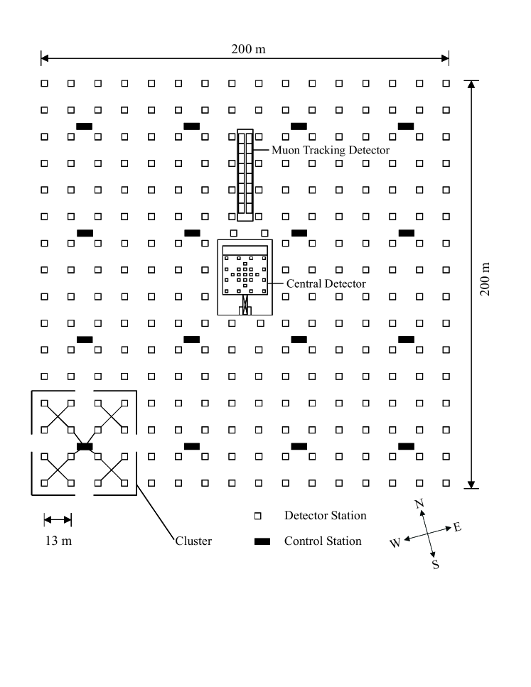
Figure 2: Schematic layout of the KASCADE experiment.

The detector installation of the experiment KASCADE (KArlsruhe Shower Core and Array DEtector) [2, 3] is located on the site of the Forschungszentrum Karlsruhe, Germany ($8^{\circ}$ E, $49^{\circ}$ N; 110 m a.s.l.). The three major components of the detector system (Figure 2) are

• an Array of scintillation detectors,

• a Central Detector: an arrangement of several different detector components, basically a hadron iron sampling calorimeter using liquid ionization chambers and

• a Muon Tracking Detector (MTD) using limited streamer tubes.

The Array covers an area of about $200\times 200\,\mathrm{m^{2}}$ and consists of 252 detector stations. These are organized in 16 clusters and placed on a square grid of 13 m separation. The detector stations contain liquid scintillation counters ($e/\gamma$ detectors) of $0.79\,\mathrm{m^{2}}$ area each and plastic scintillators of $0.81\,\mathrm{m^{2}}$ each ($\mu$ detectors; $E_{\mu}^{\rm thres}=230\,\mathrm{MeV}$), the latter covered by a shielding of $10\,\mathrm{cm}$ lead and $4\,\mathrm{cm}$ steel. The inner four clusters (60 stations) contain four $e/\gamma$ detectors per station but no $\mu$ detectors while the outer 12 clusters (192 stations) have two $e/\gamma$ detectors and four $\mu$ detectors per station. The reconstruction of the EAS data measured with the Array provides the basic information about lateral distributions and total intensities of the electron-photon (shower size $N_{\rm e}$) and muon components ($N_{\mu}^{\rm tr}$; see Section 4), the location of the EAS core and the direction of incidence.

The layout and performance of the Central Detector are described in reference [7]. The finely segmented hadron calorimeter is the main part of in the Central Detector system. It consists of a $20\times 16\,\mathrm{m^{2}}$ stack of about $4000\,\mathrm{tons}$ of iron with eight horizontal gaps. The calorimeter thickness corresponds to 11 interaction lengths $\lambda_{\rm I}$ for vertical hadrons. The detectors, measuring the energy deposit of the traversing charged particles, are ionization chambers filled with the room temperature liquids tetramethyl-silane (TMS) or tetramethyl-pentane (TMP), inserted into the gaps of the iron stack and read out by 40,000 electronic channels. From their signals the impact point, the direction and the energies of individual hadrons are reconstructed. In particular, the number of EAS hadrons with energies larger than $100\,\mathrm{GeV}$ ($N_{\rm h}^{E>100\,\mathrm{GeV}}$), the energy of the most energetic hadron observed in the shower ($E_{\rm h}^{\rm max}$) and the energy sum of all reconstructed hadrons ($\sum E_{\rm h}$) are deduced as shower observables (see Section 4).

A layer of 456 scintillation detectors, each with a size of $0.45\,\mathrm{m^{2}}$, is mounted in the third gap at a depth of 2.2 $\lambda_{\rm I}$. It is used for triggering the Central Detector system, for muon detection (with a threshold of $E_{\mu}^{\rm thres}=490\,\mathrm{MeV}$), and to determine arrival time distributions [8].

In the basement of the central building, below the iron stack and 77 cm of concrete, two layers of multi-wire proportional chambers (MWPCs) are arranged as a tracking hodoscope, covering an area of $122\,\mathrm{m^{2}}$ [9]. The MWPCs register muons with an energy threshold $E_{\mu}^{\rm thres}=2.4\,\mathrm{GeV}$ and provide the observable $N_{\mu}^{\star}$, i.e. number of reconstructed muons in the MWPCs. Due to the good position resolution, the MPWCs register also the spatial distribution of the high-energy muons together with traversing secondaries produced in the absorber by high-energetic hadrons, whose pattern has been shown to carry valuable information about the mass of the primary particle [10], expressed by particular parameters ($D_{-6}$, $D_{6}$) in terms of a fractal moment analysis (see Section 4).

Table 1: KASCADE detector components used in the present analysis.

Detector	Total Area	Threshold $E_{\rm{kin}}$	Observables
array $e/\gamma$	$490\,\mathrm{m^{2}}$	5 MeV	$N_{\rm{e}}$
array $\mu$	$622\,\mathrm{m^{2}}$	$230\,\mathrm{MeV}\times\sec\theta$	$N_{\mu}$, $N_{\mu}^{\rm tr}$
MWPCs	$122\,\mathrm{m^{2}}$	$2.4\,\mathrm{GeV}\times\sec\theta$	$N_{\mu}^{\star}$, $D_{-6}$, $D_{6}$
calorimeter	$320\,\mathrm{m^{2}}$	50 GeV	$N_{\rm{h}}^{E>100\,\mathrm{GeV}}$, $E_{\rm{h}}^{\max}$, $\sum E_{\rm{h}}$

Information on specific detector details is compiled in Table 1.

3 Simulations

The simulations of the EAS development, along the requirements of the analysis scheme of Figure 1, have used the air shower simulation program CORSIKA (vers. 5.62) [4]. The code incorporates several options of high-energy interaction models and is continuously under improvement. In particular, we consider the latest versions of VENUS [11], QGSJet [12] and Sibyll (vers. 1.6) [13]. VENUS and QGSJet are models based on the Gribov-Regge theory, and extrapolate the interaction features in a well defined way into energy regions which are far beyond energies available by accelerators, and especially into the extreme forward direction. Sibyll is a minijet model used as a hadronic interaction generator in the MOCCA [14] and the AIRES codes [15]. We use it here only for demonstration purposes. For the low-energy interactions CORSIKA includes the GHEISHA code [16]. The influence of the Earth magnetic field on charged particle propagation is taken into account. As density profile of the atmosphere the U.S. standard atmosphere is chosen [4].

Samples of at least 2000 proton and iron-induced showers have been simulated with all three models. Additionally for VENUS and QGSJet the intermediate mass primaries He, O and Si have been simulated. The energy distribution follows a weighted power law with a spectral index of $-2.7$ in the energy range of $10^{14}\,\mathrm{eV}$ to $3.16\cdot 10^{16}\,\mathrm{eV}$, calculated in eight intervals. The zenith angles are distributed in the range $[13^{\circ},22^{\circ}]$. The centers of the showers are spread uniformly over an area which exceeds the surface of the hadron calorimeter by 2 m on each side. In addition, roughly the same number of simulated events with the centers of the showers within the Array are used. The signals observed in individual detectors are determined by tracking all secondary particles down to observation level and passing them through a detector response simulation program based on the GEANT package [5].

4 Event reconstruction and selection

The reconstruction of the EAS observables which is described in detail in preceding publications of the KASCADE collaboration [10, 17, 18, 19, 20], applies an iterative procedure for reconstructing the shower size parameters. In a first step the shower core location is determined by a center-of-gravity technique from the energy deposit signals of all $e/\gamma$ counters, and the shower direction is estimated by a simple plane fit using the timing information of the Array detectors. In addition, as rough first approximations, the electron size $N_{\rm e}$ and muon size $N_{\mu}$ are estimated from summation of detector signals, taking into account the actual shower core position on the grid. These parameter values are initial values for the further reconstruction steps. In the second step the shower direction is determined by fitting a conical shape of the shower disc to the arrival times of the charged particle component, registered with the $e/\gamma$ counters. The lateral distributions and their shape parameters are estimated, and $N_{\mu}^{\rm tr}$ and $N_{\rm e}$ are determined.

The muon size $N_{\mu}^{\rm tr}$ is the muon content within a range of distances from the shower core between 40 m to 200 m which is the range accessible to the KASCADE experiment (the so-called truncated muon number) [20]. The lower limit is chosen to exclude contributions of the electromagnetic and hadronic punch-through near the center of the showers. The upper limit corresponds to the geometrical acceptance of the KASCADE layout. Figure 3 displays the variation of $N_{\mu}^{\rm tr}$ and $N_{\rm e}$ versus the primary energy $E$, as inferred from EAS simulations. Due to various serendipitous features of the KASCADE layout $\lg N_{\mu}^{\rm tr}$ proves to be nearly proportional to $\lg E$ and turns out to be almost independent of primary mass (Figure 3 left). This is in contrast to the electron size $N_{\rm e}$, which exhibits a strong mass dependence for fixed $N_{\mu}^{\rm tr}$ as shown in Figure 4 (right).

Contributions to the detector signals of other particles than electrons and muons are eliminated by applying a lateral energy correction function to appropriate particle densities, which are fitted with a likelihood function to the Nishimura Kamata Greisen (NKG) formula [21, 22]. Values of the radius parameters of 89 m and 420 m for electrons and muons, respectively, are used [17]. For showers whose cores are located within 91 m from the Array center, the reconstruction uncertainty is about 2 m for the location of the shower center, $0.5^{\circ}$ for the angle of incidence, and less than 10% and 20% for $N_{\rm e}$ and $N_{\mu}^{\rm tr}$ values, respectively, at primary energies larger than $10^{15}\,\mathrm{eV}$.

Figure 3: The mean values of the truncated muon number $N_{\mu}^{\rm tr}$ and electron number $N_{\rm e}$ vs. primary energy as inferred on basis of the indicated interaction models. For sake of clarity only QGSJet predictions are fitted by a linear function in lg-lg scale, in order to emphasize the much more pronounced mass dependence of the shower size $N_{\rm e}$.

Muon tracks observed with the MWPCs, reconstructed from pairs of hits in the two MWPC layers (vertically separated by 38 cm [10]), are summed up to obtain $N_{\mu}^{\star}$. A limit for the reconstructed angle of $\pm 15^{\circ}$ in zenith and $\pm 45^{\circ}$ in azimuth with respect to the shower axis determined from the Array is imposed (the azimuth cut is not applied for showers with zenith angles of $<10^{\circ}$). The analysis of the number and spatial distribution of the muons and of produced secondaries in terms of two generalized multi-fractal dimensions $D_{-6}$ and $D_{6}$ is discussed in [10]. These parameters characterize the spatial distribution of muons and high-energy (punch-through) hadrons as well as the degree of fluctuations of particles in the shower core.

The reconstruction of the hadronic shower variables applies appropriate pattern recognition algorithms [18, 19]. Energy clusters found in different detector layers are traced from lower layers to the topmost one to form a particle track. Additionally, the angle of incidence of the track can be deduced by the same procedure starting at lower layers, patterns of cascades have to form clusters from the remaining energy bunching up to showers according to the already determined direction. Furthermore, signals in the first layer from the top are not used for energy determination, because their electromagnetic punch-through distorts the hadron signals. The signals, weighted by the overlying absorber thickness are summed up and converted to hadron energies [7]. Similar to the shower size $N_{\rm e}$, the reconstructed number of hadrons ($N_{\rm h}^{E>100\,\mathrm{GeV}}$) exhibits a strong mass dependence for fixed $N_{\mu}^{\rm tr}$ as well (Figure 4; right).

For the investigation of the primary energy spectrum and mass composition, as well as of particular correlations of observables, two sets of data are compiled.

Figure 4: The variation of the mean values of the electron shower size (left) and number of reconstructed hadrons $N_{\rm h}^{E>100\,\mathrm{GeV}}$ (right) with $N_{\mu}^{\rm tr}$. The predictions of different models for proton and iron induced showers are compared with results of the measurements.

One set - further referred to as selection I - uses the information of electrons and muons from the Array stations only. It allows analysis the data with good statistical accuracy, but includes only little information provided by the Central Detector. A second data set - henceforth referred to as selection II - includes observables measured in the Central Detector, but this data sample comprises only a small amount of registered showers. Selection I comprises 720,000 EAS events, accumulated in 226 days, with primary energies larger than $E\approx 5\cdot 10^{14}\,\mathrm{eV}$ and with a maximum core distance from the center of the Array of 91 m and with angles of incidence in the range of $[13^{\circ},22^{\circ}]$. Selection II comprises approximately 8000 high-energy, central showers selected by cuts on $N_{\mu}^{\rm tr}$ ($\lg N_{\mu}^{\rm tr}>3.5$), on the core location ($R_{\rm core}<5\,\mathrm{m}$ from the center of the Central Detector), with at least one reconstructed hadron of an energy above 100 GeV and 10 muons observed in the MWPCs.

5 Non-parametric analyses

The present analysis of mass composition and energy spectrum avoids the bias inherent in parametric procedures and is performed for individual events by use of multivariate non-parametric Bayesian and neural network decision methods. In this way we are able to specify, in a transparent and coherent way, how conclusive and trustworthy our results are, as expressed by true classification and misclassification matrices of the results. A brief outline and more details of the applied methods are given in Appendix A and in reference [23].

The combination of the total muon content $N_{\mu}$ and the shower size $N_{\rm e}$ has been shown to be sensitive to primary mass and is applied in numerous experimental studies, using suitable parameterizations of the predicted $\lg N_{\mu}/\lg N_{\rm e}$ relation with the primary mass. However, as indicated above, the total muon content $N_{\mu}$, although displaying some dependence on primary mass, is a quantity not easily accessible experimentally without additional assumptions about the shape of the lateral muon density distribution at large distances from the shower core. Therefore, we prefer to consider the truncated muon number $N_{\mu}^{\rm tr}$, which - on average - proves to be nearly independent from primary mass (see Figure 3), but it is, on the other hand, a rather sensitive energy identifier. Thus, at fixed $N_{\mu}^{\rm tr}$, the information about the mass is essentially provided by the shower size $N_{\rm e}$ [20]. In cases of other EAS observables mass and energy sensitivities are, in general, less well marked, and in principle, each shower variable carries information simultaneously on mass and energy in a way which is additionally affected by the considerable fluctuations of the shower development. The most sensitive EAS observables, $N_{\rm e}$ and $N_{\mu}^{\rm tr}$, display the smallest intrinsic and sampling fluctuations.

5.1 Mass composition

Due to the limited number of simulated EAS and the correspondingly limited statistical accuracy it is hardly reasonable to use the full set of observables simultaneously to achieve a reliable result about mass composition (curse of dimensionality condition; see Appendix A). Hence we consider simultaneously only a few observables.

Each simulated or measured event is represented by an observation vector $x=(N_{\rm e},N_{\mu}^{\rm tr},\ldots)$ of the $n$ observables. Applying the technique described in Appendix A the likelihood (probability density distribution) $\hat{p}(x|\omega_{i})$ of an event for each class $\omega_{i}\in\{{\rm p,O,Fe}\}$ can be calculated, i.e. the probability of an event $x$ belonging to a given class $\omega_{i}$.

As an example, the superposition of the estimated probability density distributions, referring to two sets of different observables, are displayed in Figure 5 (based on QGSJet simulations). The regions where $\hat{p}(x|\omega_{\rm p})$, $\hat{p}(x|\omega_{\rm O})$ and $\hat{p}(x|\omega_{\rm Fe})$ are larger than the other two possibilities are colored light, middle and dark grey, respectively. The left graph shows the density distribution calculated in the two dimensional space of the observables $N_{\rm e}$ and $N_{\mu}^{\rm tr}$. A rough separation can be recognized, but also a strong overlapping of the likelihood distributions has to be admitted.

The right-hand graph of Figure 5 shows an example of two observables ($N_{\mu}^{\star}$ and $N_{\mu}^{\rm tr}$), which exhibit only weak mass-discrimination power. Correspondingly, the density distributions of the three particle types are intermixed, and reliable conclusions could not be drawn. In case of selection II the mass composition is reconstructed for different sets of observables using the Bayes theorem (Equation 2). When the estimated posterior probability $\hat{p}(\omega_{i}|x)$ is larger than $\hat{p}(\omega_{j}|x)$, then the event is assigned to class $\omega_{i}$, otherwise to class $\omega_{j}$. Taking into account (by Equation 2) the estimated number of incorrectly classified events (i.e. misclassification rates) (Table 2) the true proportions of the different particle types are reconstructed.

The classification rates $P_{ij}=\hat{P}_{\omega_{i}\rightarrow\omega_{j}}$ (see Appendix: Equation A.1 and Figure 14) give the fraction of correctly, $P_{ii}$, and wrongly, $P_{ij}$, classified events with $i\neq j$, an example for three mass class is given in Table 2. Of course, the sum of each row has to be 100%.

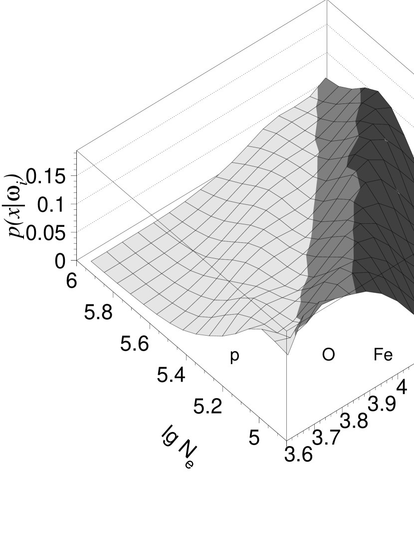
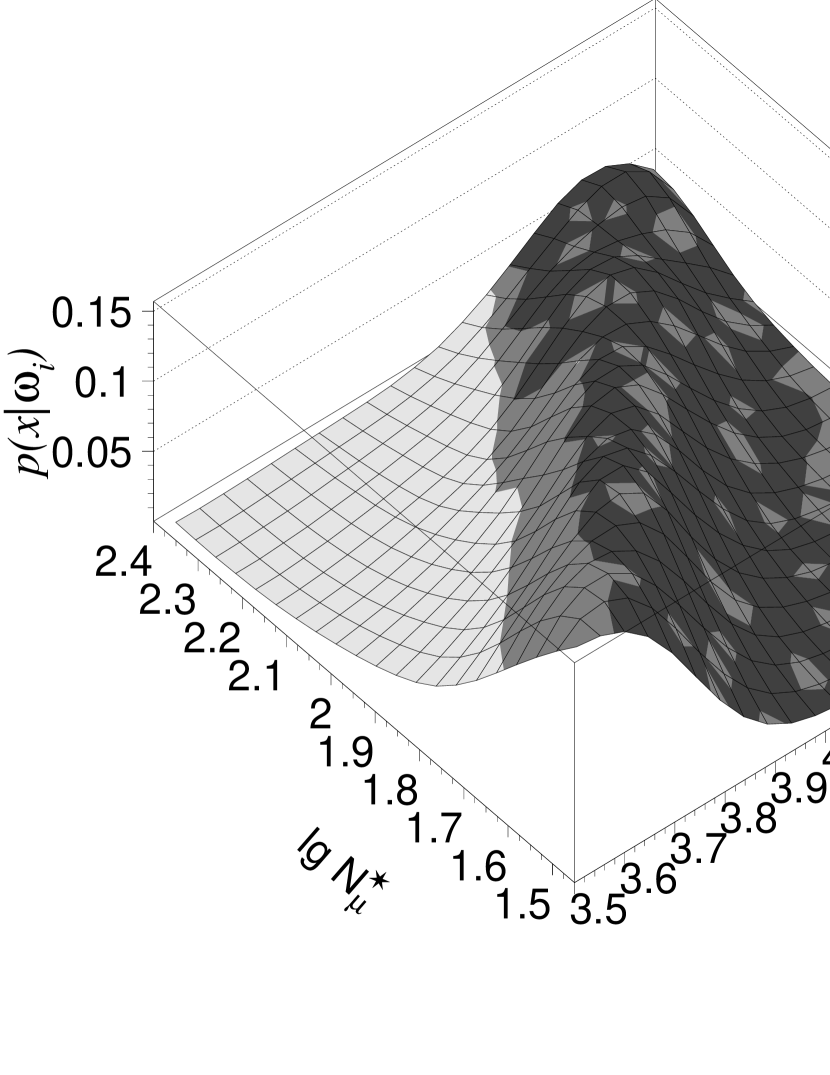
Figure 5: Superposition of three probability density distributions $\sum_{i=1}^{3}\hat{p}(x|\omega_{i})/3$ deduced from QGSJet simulations using the observables $N_{\rm e}$ and $N_{\mu}^{\rm tr}$ (left) as well as $N_{\mu}^{\star}$ and $N_{\mu}^{\rm tr}$ (right). Events in the dark shaded area mark the region classified as iron, middle grey as oxygen, and light grey as proton (selection II).

Table 2: Classification matrices for three classes (p, O and Fe) and two different models. In addition to the classification rates of p, O and Fe, the rates of classified intermediate groups He and Si respectively, are given. The used observables are $N_{\mu}^{\rm tr}$ and $N_{\rm e}$ ($3.6\leq\lg N_{\mu}^{\rm tr}<3.9$).

	QGSJet			VENUS
$\hat{P}_{\omega_{j}\rightarrow\omega_{i}}$ [%]	$\omega_{i}=$p	$\omega_{i}=$O	$\omega_{i}=$Fe	$\omega_{i}=$p	$\omega_{i}=$O	$\omega_{i}=$Fe
$\omega_{j}=$p	$77\pm 3$	$21\pm 3$	$2\pm 1$	$78\pm 3$	$21\pm 2$	$1^{+2}_{-1}$
$\omega_{j}=$He	$57\pm 3$	$39\pm 3$	$4\pm 1$	$64\pm 3$	$32\pm 2$	$4\pm 1$
$\omega_{j}=$O	$14\pm 2$	$61\pm 3$	$25\pm 3$	$15\pm 2$	$61\pm 4$	$24\pm 3$
$\omega_{j}=$Si	$3\pm 1$	$54\pm 3$	$43\pm 2$	$3\pm 2$	$51\pm 3$	$46\pm 2$
$\omega_{j}=$Fe	$1\pm 1$	$17\pm 2$	$82\pm 3$	$0^{+1}_{-0}$	$20\pm 3$	$80\pm 3$

In the most probable cases the different particle types are identified correctly, but the knowledge of the incorrectly classified events could be used for a correction due to the mis-classification. In addition, the rates for the intermediate mass particle types, He and Si, are given. Helium is mostly classified as protons (57%) and silicon as oxygen (54%). Due to the stronger fluctuations and weaker correlations with mass and/or energy, different sets of observables result in lower true-classification rates $P_{ii}$. In general, if the rates $P_{ii}$ are less than 50%, it is no more possible to deconvolute the true proportions by matrix inversion of $P_{ij}$ (Equation 6), since the matrix $P_{ij}$ becomes singular, signaling that the determination of a class $\omega_{i}$ is just haphazard. Therefore it is not meaningful to consider more than 3 classes, since this would require an analysis of further observables simultaneously, with a number of Monte Carlo simulations larger than presently available.

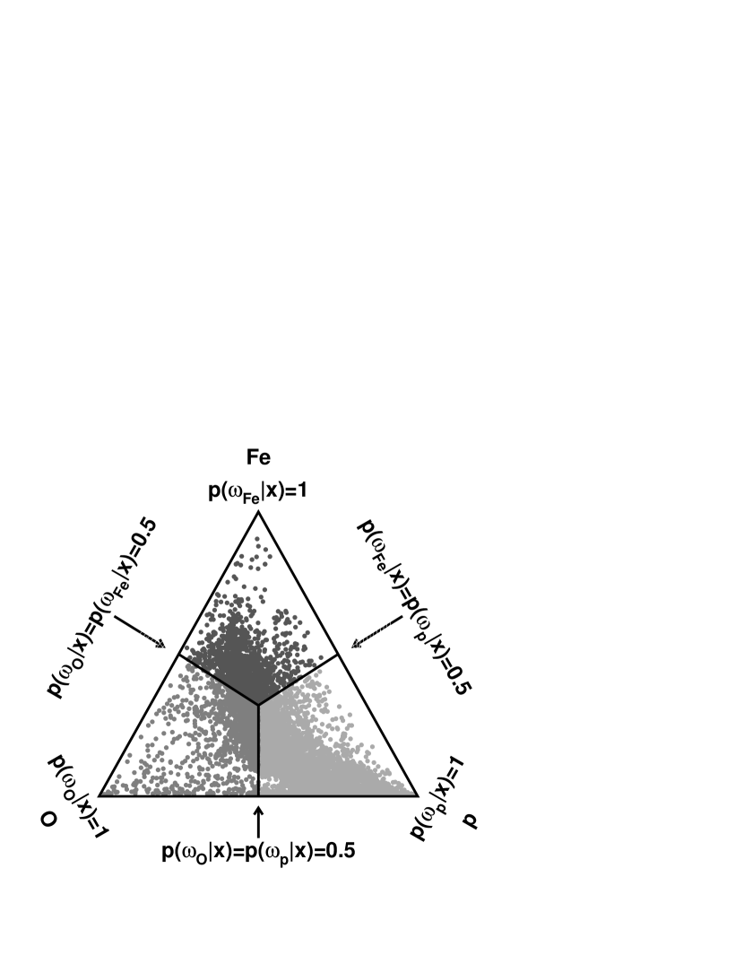
Figure 6: Estimated posterior probabilities $\hat{p}(\omega_{i}|x)$ of measured events deduced from QGSJet simulations using the observation vector $x=(N_{\rm e},N_{\mu}^{\rm tr})$ (left) as well as $x=(N_{\mu}^{\star},N_{\rm{h}}^{E>100\,\mathrm{GeV}},\sum E_{\rm{h}})$ (right).

As a cross-check the estimated posterior probabilities $\hat{p}(\omega_{i}|x)$ of a given measured event $x$, belonging to class $\omega_{i}$, can be calculated (Figure 6). The center of the triangles shown correspond to equal probability of belonging to any class, reflecting the fact that it is nearly impossible to classify the measured event, while points in the corners satisfy the relation $\hat{p}(\omega_{i}|x)=1$, i.e. the corresponding event belongs to class $\omega_{i}$ with probability unity. Hence, from given measured events we obtain information about the probabilities belonging to class $\omega_{i}$ just as well. Evidently, the set $N_{\rm e}$ and $N_{\mu}^{\rm tr}$ allows to determine a well defined mass composition. In contrast, the set comprising $N_{\mu}^{\star}$, $N_{\rm{h}}^{E>100\,\mathrm{GeV}}$, and $\sum E_{\rm{h}}$ is less suitable for mass discrimination mainly due to strong fluctuations of the observables as can be seen in Figure 6, right side.

Figure 7: The relative abundances of the classes p, O and Fe vs. $\lg N_{\mu}^{\rm tr}$, reconstructed on the basis of two different hadronic interaction models and using the EAS observables $N_{\rm e}$ and $N_{\mu}^{\rm tr}$. The right graph shows the corresponding mean logarithmic mass $\langle\ln A\rangle$ vs. $\lg N_{\mu}^{\rm tr}$. Statistical (thick lines) and methodical (thin lines) uncertainties are indicated as error bars.

Figure 8: Mean logarithmic mass $\langle\ln A\rangle$ resulting from the analysis of different sets of observables vs. $\lg N_{\mu}^{\rm tr}$ (QGSJet prediction). The sets displayed on the right do not include the observable $N_{\rm e}$. The error bars are omitted to simplify the presentation of the synopsis. The statistical errors are of the same order of magnitude as given in Figure 7. But the systematic errors are larger by $40\%-50\%$ for the data on the right graph due to a weaker correlation with mass.

The results of the composition determination, using the observables $N_{\rm e}$ and $N_{\mu}^{\rm tr}$, are given in Figure 7 as relative abundances versus $N_{\mu}^{\rm tr}$ and mean logarithmic mass $\langle\ln A\rangle$ vs. $N_{\mu}^{\rm tr}$. The mean logarithmic mass $\langle\ln A\rangle$ cannot be calculated unambiguously because only abundances of groups of elements can be determined. We have assigned $\langle A_{\rm p+He}\rangle=2.5$, $\langle A_{\rm O}\rangle=16$, $\langle A_{\rm Si+Fe}\rangle=42$ to the p, O and Fe group, respectively. This procedure is of course to some extent arbitrary, but this is always implicit, when $\langle\ln A\rangle$ is used. The statistical errors (thick lines) are calculated according to a multinomial distribution. The thin error bars correspond to a methodical uncertainty, calculated by the bootstrap method (see Appendix A). It reflects the influence of the limited number of Monte Carlo events. Apparently the use of the VENUS model results in a lighter composition, compared with the use of QGSJet. A tendency towards a heavier composition above the knee ($\lg N_{\mu}^{\rm tr}=4.15$ corresponding to $4\,\mathrm{PeV}$) is indicated, albeit the statistical and systematic uncertainties do not allow a definite conclusion and the results are clearly compatible with an energy independent composition.

Results of several other combinations of observables by using the QGSJet model are summarized in Figure 8. In general, the tendencies are the same. Remarkably, all sets omitting the electron size $N_{\rm e}$ (right graph) result in a heavier composition and a more pronounced increase above the knee. As the electron size has the strongest mass sensitivity, as well as the smallest fluctuations, the mass compositions are predominantly determined by $N_{\rm e}$ and $N_{\mu}^{\rm tr}$ (left). Compositions resulting from sets of less sensitive observables differ from these values (right). The tendencies are quite similar for the VENUS model, but the absolute values are shifted towards a lighter composition as expected from Figure 7.

The fact that different combinations of observables taken into account in the analysis, lead apparently to different mass compositions (shown in Figure 8), reveals inadequacies of the reference model, i.e. that the degree of the intrinsic correlations of different observables differs from those of the real data. Otherwise the determined mass compositions should be identical within the statistical errrors.

5.2 Energy spectra

To estimate the primary energy $E$ the most important parameters are $N_{\rm e}$ and $N_{\mu}^{\rm tr}$ again, where now $N_{\mu}^{\rm tr}$ carries most of the information. As data basis we use selection I. Due to the large computing time requirements we do not apply the Bayesian algorithms here and use instead neural networks only. In principal there are no basic arguments to prefer one particular method. Previous publications have demonstrated the consistency and equivalence of neural network and Bayesian methods in EAS analyzes [24, 25]. The neural networks employed have typically a simple net topology $2\times 5\times 2\times 1$, but several other topologies have been used to estimate the methodical error of this special choice. For training the network (according to Equation 8) two independent samples have been generated to allow a validation of the results (Appendix A).

Figure 9: The relative error vs. primary energy for different classes: Results obtained with a network trained with QGSJet samples (left) and the result of the same network analyzing VENUS samples (right).

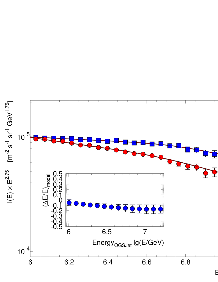
Figure 10: Differential energy spectra resulting from the analysis of data of the KASCADE experiment using two differently trained networks (by VENUS and QGSJet samples). The reconstructed energies are compared on an event-by-event basis and their differences are given in the inset as relative error vs. the energy reconstructed on the basis of the QGSJet model.

Before data analysis, the response and the biases of the trained neural network have to be carefully scrutinized. For this, the performance of mass classification and energy estimation has been investigated with the other MC sample as input. We consider the relative deviation of the reconstructed energy $E_{\rm est}$ from the true value $E_{\rm true}$, which is known for the simulated samples, more precisely, the distribution of $\Delta E/E=(E_{\rm est}-E_{\rm true})/E_{\rm true}$, whose mean value and the standard deviation represent the bias and the energy resolution (relative error) of the reconstruction, respectively.

Figure 9 displays the relative error of the estimated energy for different primary particles. The relative error of a network, trained with QGSJet samples, is shown in the left part. In general, the bias for the various classes is less than 3-5%, but the energy resolution (spread) proves to be strongly mass dependent. As expected, the iron class has the smallest energy spread ($\sigma_{Fe}\approx 21\%$ versus $\sigma_{p}\approx 38\%$). The network trained with VENUS samples leads to the same results. Also shown (right) are the results of a network, which has been trained with QGSJet samples analyzing events generated with the VENUS model. With increasing energy the QGSJet trained network underestimates systematically the true energy of the VENUS samples. Moreover, the bias appears to be mass dependent, implying that the degree of the correlation between energy and the analyzed shower observables is varying differently for the different primary particles and models. This is a caveat to the estimate of true energies of the measured event samples, namly that hidden mass dependent correlations lead to an all-particle spectrum depending on the true mass composition.

Figure 10 presents the reconstructed energy spectra of measured data resulting from the analysis using two different networks, trained with QGSJet and VENUS samples. Apparently, the VENUS trained network results in a steeper spectrum as compared with the QGSJet findings. It should be emphasized that the network used takes into account not only the absolute values of the observables $N_{\rm e}$ and $N_{\mu}^{\rm tr}$, but also their correlations. In order to specify the relative error arising from the model dependence, mean value and spread of $\left(\Delta E/E\right)_{model}=(E_{\rm VENUS}-E_{\rm QGSJet})/E_{\rm QGSJet}$ are additionally given (inset). The variation of this model error displays a change at higher energies, which might indicate a change of the composition.

The resulting spectra are fitted by the trial function (see Figure 10)

$$I(E)=I_{0}\cdot\left(\frac{E}{E_{\rm knee}}\right)^{-\gamma_{1}}\cdot\left(1+\left(\frac{E}{E_{\rm knee}}\right)^{\varepsilon}\right)^{\frac{\gamma_{1}-\gamma_{2}}{\varepsilon}}$$ (1)

Table 3: Comparison of parameters of the energy spectrum, derived on basis of on the VENUS and QGSJet simulations, respectively. The first error is the statistical one. The second error represents the systematic uncertainty resulting from the small number of simulated event.

	QGSJet			VENUS
$\gamma_{1}$	2.77 $\pm$	0.003 $\pm$	0.03	2.87 $\pm$	0.003 $\pm$	0.04
$\gamma_{2}$	3.11 $\pm$	0.02 $\pm$	0.06	3.25 $\pm$	0.02 $\pm$	0.06
$E_{\rm knee}$ [$10^{6}\,\mathrm{GeV}$]	5.5 $\pm$	0.2 $\pm$	0.8	4.5 $\pm$	0.3 $\pm$	0.9
$\chi^{2}/dof$	0.95			1.94

which accounts for a smoothly changing power law spectrum [26]. The parameter $\varepsilon$ controls the width of the transition region, and the

Figure 11: The differential all-particle cosmic ray flux obtained here compared to the results reported by Tibet AS$\gamma$ [29], Akeno [30], and CASA-MIA [27]. The data points are multiplied by $(E/GeV)^{2.5}$. Only statistical errors are presented.

knee position $E_{\rm knee}$ is defined by the center point of the transition region. Asymptotically $I(E)$ approaches to power law functions $E^{-\gamma_{1},\gamma_{2}}$. The parameter uncertainties have been studied by calculating the errors $I(E)\pm\Delta I(E)$ using the sampling correlation matrix. But the resulting error bands are so narrow that it does not visibly differ from the $I(E)$-line. The best-fit results are given in Table 3, including statistical errors as well as the methodical error derived from different training parameters of the neural network. It is obvious that the statistical errors are considerably smaller than the systematic uncertainties resulting from the small number of simulated events and from interaction models.

Figure 11 compares the spectra of Figure 10 with results reported by other experiments. All measurements, independently from each other, show a steepening above a particular energy: the knee. But the absolute intensity of the flux and the position of the knee obviously differ. This is most likely due to different model assumptions or energy conversion functions used. The considerable deviation between CASA-MIA [27] and the other two experiments may be explained in this way. CASA-MIA used the Sibyll model for constructing an energy estimator $E=f(N_{\rm e},N_{\mu})$ from the electron and muon sizes. The fact that Sybill predicts significantly lower values of $N_{\mu}$ and larger values for $N_{\rm e}$ [28] as compared to QGSJet and VENUS, could lead to a systematic shift of the spectrum towards lower energies. In view of the considerable model dependence of our results, the overlap with some of the other experiments should not be taken as evidence for or against any of them.

5.3 Combined analysis of energy and mass

As an example, Figure 12 shows the relative abundances of a mass classification into three categories, as well as the corresponding mean logarithmic mass, resulting from the analysis of central showers (selection II) vs. the estimated energy. The observables $N_{\rm e}$ and $N_{\mu}^{\rm tr}$ are used as input parameters. Again, the VENUS model leads to a lighter mean logarithmic mass in the considered energy range as compared to the QGSJet model. Besides the Bayesian method a neural network analysis was performed additionally. The network results are denoted by NN. Within the statistical errors the mass composition resulting from both pattern recognition procedures agree. Our data reveal a mixed composition, becoming lighter when approaching the knee and heavier above the knee. This feature appears to be somehow mysterious, but the tendency is supported by recent results of the CASA-BLANCA [31] and HEGRA [32] experiments. In fact, there are also astrophysical arguments for a minimum of the mean mass in the range of the knee [33].

Figure 12: Relative abundances reconstructed by Bayes classification vs. the reconstructed energy based on the QGSJet model and using $N_{\rm e}$ and $N_{\mu}^{\rm tr}$. Additionally, the corresponding mean logarithmic mass $\langle\ln A\rangle$ (right; Bayes) and the corresponding variation resulting from the neural network analysis (NN) are given. The error bars represent the statistical (thick) and methodical (thin) uncertainties.

In the present status of our analysis procedure it is hardly possible to introduce more than three classes for the reconstruction of the mass composition. If this were to be attempted additional observables had to be included. A finer binning of the energy scale (beyond the energy resolution $(\Delta E/E)_{\rm est}$) for the spectra of single masses would require to deconvolute the resolution effects. In the actual analysis this step has not been performed and only a few representative values of the varying mass composition (and no detailed energy spectra of the different mass classes) have been presented. To analyze the data beyond this limit we need, in the simplest case, to construct from the misclassification matrices a matrix $A_{\rm AA^{\prime};EE^{\prime}}$ deconvoluting mass and energy resolution effects. Stressing once more the curse of dimensionality (see Appendix A), a very large number of simulated events is required for the determination of such a matrix (at least 150000 simulated events are needed). For the same reasons we are presently unable to infer any significant fine structure from the all-particle energy spectrum beyond the resolution $(\Delta E/E)_{\rm est}$.

Different sets of observables lead to different mass compositions. This feature may indicate that not only the absolute values, but also the correlations of the observables are not described satisfactorily by any of the models. Nonetheless, a reduced model dependence can be observed when a well marked relation is projected out from the correlations of the multivariate distribution.

Figure 13: The projected relations $\lg N_{\rm e}$ and $\lg N_{\rm h}^{E>100\mathrm{GeV}}$, respectively, vs. $\lg(E/\mathrm{GeV})$ from two neural networks, trained to estimate the energy and mass of the measured events using $N_{\rm e}$ and $N_{\mu}^{\rm tr}$ as EAS observables.

Figure 13 displays on the left-hand side the relation between electron size $N_{\rm e}$ and energy $E$, which shows no difference between simulated and measured samples. Of course, this is not surprising, since the pattern recognition tool is just trained in that way, such that deviations, incompatible with the statistical accuracy, would cast some methodical doubts on the used algorithms. More remarkable is the agreement of $N_{\rm h}^{E>100\,\mathrm{GeV}}$ vs. primary energy, found by the same network though with larger fluctuations of the mean values. That may be explained by the reduced mass sensitivity of $N_{\rm h}^{E>100\,\mathrm{GeV}}$ and the dominance of the $N_{\rm e}$-$N_{\mu}^{\rm tr}$ correlation (compare the observable sets in Figure 8 left). Nevertheless, within the statistical significance level (in terms of hypotheses tests like student $t$-test) no difference between data and model predictions can be stated.

6 Discussion and conclusion

The present paper aims at presenting methods of a determination of primary energy spectrum and mass composition of cosmic rays in the energy range $10^{15}-5\cdot 10^{16}\,\mathrm{eV}$ by an event-by-event analysis of EAS data. The specific methodical feature is the use of a non-parametric approach, studying multivariate distributions of a number of EAS observables [34, 25].

The present approach to obtain information about the EAS primaries has following merits:

• It specifies the inevitable model dependence of any statement about spectrum and mass composition, introduced through the patterns provided by the Monte Carlo simulations on basis of a particular hadronic interaction model.

• The model dependence is not only revealed by the results from the analysis of single EAS observables when comparing different hadronic interaction models, but the approach specifies also the degree of correlations between different observables used for the multivariate analysis.

• This feature provides the possibility to test a specific hadronic interaction model by exploring the internal consistency of the results, when the outcome of different sets of observables are considered. This aspect is of greatest importance for approaching the best model reproducing the observations in the most consistent way.

• Comparing the KASCADE findings with other experiments shows that the discrepancies between results can well be attributed to the different interaction models employed.

Appendix A Non-parametric statistical inference

Pattern recognition techniques are efficient tools to determine the correct association of a given sample to a certain category or class. From the measurements or simulations of a physical phenomenon, a set of quantities (observables) is obtained, like $N_{\mu}^{\rm tr}$ or $N_{\rm e}$, which defines an observation vector $x$. This observation vector serves as the input to a procedure based on decision rules, by which a sample is assigned to one of the given classes. Thus it is assumed that an observation vector is a random vector $x$ whose conditional density function $p(x|\omega_{i})$ depends on its class $\omega_{i}$ (e.g. p, O and Fe classes).

In the following we consider so called non-parametric techniques like Bayes classifiers and artificial neural networks [6]. The term non-parametric indicates that the representations of the distributions (like probability density functions of Bayes classifiers or weights of neural networks) are no more specified by a-priori chosen functional forms. They are constructed through the analysis process by the given data distributions themselves.

It should be immediately emphasized that there are some important limitations. In case of a finite set of random samples, the dimension $n$ of the random vector $x$ is limited by the following condition: When considering each component of an $n$-dimensional observation vector by $M$ divisions, the total number of cells is $M^{n}$ and is increasing exponentially with the dimensionality of the input space. Since each cell should contain at least one data point this requirement implies that the size of training samples (or reference pattern samples) needed to specify the non-parametric mapping, is increasing correspondingly. This condition is called the curse of dimensionality [35] and prohibits the simultaneous (multivariate) analysis of a larger number of EAS observables, when the size of training samples is too small.

A.1 Bayesian decision rule

The Bayes classifier is a powerful algorithm but time consuming with large memory requirements. However, its performance is generally excellent and asymptotically Bayes optimal, so that the expected Bayes error (see below) is less than or equal to that of any other technique [36]. The estimated probability densities converge asymptotically to the true density with increasing sample size [37, 38].

The method is based on the Bayes Theorem [39]

$$p(\omega_{i}|x)=\frac{p(x|\omega_{i})\times P(\omega_{i})}{p(x)}\quad\Leftrightarrow\quad\mbox{posterior}=\frac{\mbox{likelihood}\times\mbox{prior}}{\mbox{normalization factor}}$$ (2)

with $p(x)=\sum_{j=1}^{N}p(x|\omega_{j})P(\omega_{j})$, which holds if the different $N$ hypotheses $\omega_{i}$ (i.e. classes) are mutually exclusive and exhaustive. By a prior and a normalization factor the theorem connects the likelihood for an event $x$ of a given class $\omega_{i}$ with the probability of a class $\omega_{i}$, being associated to a given event $x$. The prior gives the a priori knowledge of the relative abundance of each class and is major basis of debates on Bayesian inference procedures. It is nearly always the best to follow the advice given by Bayes himself [39], generally known as Bayes’ Postulate (occasionally also referred to as Principle of Equidistribution of Ignorance): So far there exists no further knowledge, the prior probabilities should be assumed to be equal

$$P(\omega_{i})=\frac{1}{N}\quad\mbox{ with }\quad\sum_{i=1}^{N}P(\omega_{i})=1$$ (3)

In the fortuitous case that the likelihood functions $p(x|\omega_{i})$ are known for all populations, the Bayes optimal decision rule is to classify $x$ into class $\omega_{i}$, if

$$p(\omega_{i}|x)>p(\omega_{j}|x)$$ (4)

for all classes $\omega_{j}\neq\omega_{i}$, as illustrated (with the mis-classification probabilities) in Figure 14.

To construct an estimate $\hat{p}(x|\omega_{i})$ of the likelihood $p(x|\omega_{i})$ of class $\omega_{i}$, the $k$-th simulated event $x_{ki}$ is assumed to have a sphere-of-influence where it contributes to the probabilities (see Figure 14). There are various procedures to specify these contributions whose superpositions lead to continuous likelihood functions, replacing the frequency distributions of discrete simulated events $N_{i}$ of each class $\omega_{i}$ in the $n$-dimensional observation space. A standard choice of such spheres are multivariate normal distributions, because they are simple, well behaved, easily computed and have been shown in practice to perform well:

$$\hat{p}(x|\omega_{i})=\frac{1}{N_{i}}\sum_{k=1}^{N_{i}}\frac{1}{(\sqrt{2\pi}\sigma)^{n+1}\sqrt{|C_{i}|}}\exp\left(-\frac{1}{2\sigma^{2}}||x-x_{ki}||\right)$$ (5)

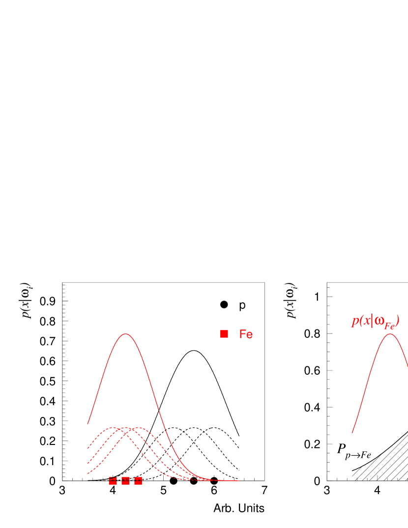
Figure 14: Schematic illustration of the construction of two one-dimensional (overlapping) likelihood functions $p(x|\omega_{\rm p,Fe})$, approximated by Gaussian distributions (sphere-of-influence) for each event, indicated on the abscissa (left). Classification using the Bayes decision showing the proportion of mis-classified events by the hashed areas (right) ($P(\omega_{Fe})=P(\omega_{p}))$ .

The Mahalanobis metric $||x-x_{ki}||=(x-x_{ki})^{T}C_{i}^{-1}(x-x_{ki})$ is used, because the observables are transformed to unit variances by the sampling covariance matrix $C_{i}$ for each class $\omega_{i}$, resulting in equal importance of all components.

The scaling parameter $\sigma$ controls the width of the sphere-of-influence and is obtained by the median of an ordered statistics of estimated Bayes errors for different initial values of $\sigma$ [23]. The Bayes error $\epsilon$ represents the total sum (integral) of mis-classified events and is given in case of two classes by the simple relation $\epsilon=\int\min\{p(\omega_{1}|x),p(\omega_{2}|x)\}\cdot p(x)\d x$ (hatched areas in Figure 14 right). To account for the mis-classification, the rates $P_{ij}=P_{\omega_{i}\rightarrow\omega_{j}}$, i.e. the probability of an event $x\in\omega_{i}$ being classified in the class $\omega_{j}$, are estimated by the leave-one-out method (also called jack-knifing). Each simulated event is held back once while the others are used to estimate the association of this particular event. By a, so called, bootstrap method different subsets of each simulated class are used to perform the leave-one-out method to give an asymptotically unbiased estimate of the variance of the $\hat{P}_{ij}$ [36]. Thus the true number of events $n_{i}^{\star}$ can be deduced from the classified events $n_{j}$ by a matrix inversion:

$$\sum_{j}\hat{P}_{ij}^{-1}n_{j}=n_{i}^{\star}\qquad\mbox{ with }\quad\hat{P}_{ij}=\hat{P}_{\omega_{i}\rightarrow\omega_{j}}$$ (6)

A.2 Neural networks

An artificial neural network can be considered as a nonlinear transfer function

$$f:\Rset^{p}\longrightarrow\Rset^{q}$$ (7)

mapping a bounded euclidian space of dimension $p$ to another space of dimension $q$. The, so called, multilayer feed-forward neural network is organized in $L$ different layers: an input layer, $L-2$ hidden layers, and an output layer. Each layer $l$ consists of a certain number $n_{l}$ of units (neurons), which carry on the signals to the next layer. The, so called, network topology specifies the number of units in each layer: $n_{1}\times n_{2}\times\ldots\times n_{L-1}\times n_{L}$. An output unit $y_{mL}$ of the output layer $L$ is determined for each observation vector (input units) $x_{ki}$ and class $\omega_{i}$ entering the input layer and should be close to the true value $t_{ki}$, given by the labeled simulation events in terms of a well defined measure. Thus, the error function $E({\bf w})$

$$E({\bf w})=\frac{1}{2}\sum_{i=1}^{N}\frac{1}{N_{i}}\sum_{k=1}^{N_{i}}\left(y_{mL}(x_{ki},{\bf w})-t_{ki}\right)^{2}$$ (8)

has to be minimized. For each layer $l$, except of the input, the outcome of each neuron $m$ is calculated by a weighted sum of the output of neurons of the last preceding layer. Additionally an activation function $f(z)$ is applied to the sum

$$y_{ml}=f(z)=f\left(\sum_{i=1}^{n_{l-1}}w_{i,l-1}^{m}\cdot y_{i,l-1}+w^{m}_{l}\right).$$ (9)

A convenient practice is to use the Fermi function $f(z)=1/(1+\exp(-z))$. The most common algorithm for the network training, i.e. minimizing $E({\bf w})$, is an adjustment of the weights $w_{i,l-1}^{m}$ and $w^{m}_{l}$ by a stochastic minimization procedure [23] or alternatively by the, so called, back-propagation algorithm [40]. There exist different other algorithms or extended versions of this basic back-propagation, which try to circumvent problems in finding the global minimum or sticking in a local minimum. Additional problems arise, if the training process leads to an overtraining of the network by adopting the properties of the training samples, but cannot give satisfactory results, when it is applied to another validation set. Thus, in a generalization phase one has to control the quality of the network with an independent labeled set of samples.

In general, the output $y_{mL}$ is a continuous function. Hence not only the classification can be done applying neural networks, but also parameter estimation (regression) is possible, e.g. the estimation of the primary energy of EAS events. In case a classification into $N$ classes is required, the output $y_{mL}$ of the network is divided into $N$ regions, each representing a single class [23].

In previous publications the consistency and equivalence of neural network and Bayes classifier results in EAS analysis have been demonstrated [24, 25]. The classification rates $P_{ij}$ inferred from both procedures do not differ significantly. Thus, an adequate choice of the particular decision rule and of the appropriate algorithm is just a matter of the actual conditions like computing time and memory workload.

References

- [1] G.V. Kulikov and G.B. Khristiansen, Soviet Physics JETP 35 (1959) 441.
- [2] P. Doll et al., KfK-Report 4686, Kernforschungszentrum Karlsruhe 1990.
- [3] H.O. Klages et al., Nucl. Phys. B (Proc. Suppl.) 52B (1997) 92.
- [4] D. Heck et al., FZKA-Report 6019, Forschungszentrum Karlsruhe 1998.
- [5] CERN Program Library Long Writeups W5013 1993.
- [6] A.A. Chilingarian, Comput. Phys. Commun. 54 (1989) 381.
- [7] J. Engler et al., Nucl. Inst. Meth. A 427 (1999) 528.
- [8] T. Antoni et al., (KASCADE Collaboration), ”Time Structure of the EAS Muon Component measured by the KASCADE Experiment”, Astropart. Phys., in press.
- [9] H. Bozdog et al., ”The detector system for measurement of multiple cosmic muons in the central detector of KASCADE”, Nucl. Inst. Meth., submitted.
- [10] A. Haungs et al., Nucl. Inst. Meth. A 372 (1996) 515.
- [11] K. Werner, Phys. Rep. 232 (1993) 87.
- [12] N.N. Kalmykov, S.S. Ostapchenko, Yad. Fiz. 56 (1993) 105.
- [13] J. Engel et al., Phys. Rev. D 50 (1994) 5013.
- [14] A.M. Hillas, Proc. Int. Cosmic Ray Conference, Paris 8 (1981) 193.
- [15] S. Sciutto, ”AIRES a System for Air Shower Simulations-Version 2.2.0”, Auger Project Report GAP-99-044, 1999.
- [16] H. Fesefeldt, Report PITHA 85/02, RWTH Aachen, Germany 1985.
- [17] T. Antoni et al., (KASCADE Collaboration), Astropart. Phys. 14 (2001) 245.
- [18] J. Unger et al., Proc. Int. Cosmic Ray Conference, Durban 6 (1997) 145; J. Unger, FZKA-Report 5896, Forschungszentrum Karlsruhe 1997, in German.
- [19] J.R. Hörandel, FZKA-Report 6015, Forschungszentrum Karlsruhe 1998, in German.
- [20] J.H. Weber et al., Proc. Int. Cosmic Ray Conference, Durban 6 (1997) 153; J.H. Weber, FZKA-Report 6339, Forschungszentrum Karlsruhe 1999, in German.
- [21] K. Greisen, Progress in Cosmic Ray Physics 3, North Holland Publ. 1956.
- [22] K. Kamata, J. Nishimura, Prog. Theoret. Phys. Suppl. 6 (1958) 93.
- [23] A.A. Chilingarian, ANI users guide, unpublished.
- [24] M. Roth, FZKA-Report 6262, Forschungszentrum Karlsruhe 1999, in German.
- [25] A.A. Chilingarian et al., Nucl. Phys. B (Proc. Suppl.) 52B (1997) 237.
- [26] S.V. Ter-Antonyan, L.S. Haroyan, preprint hep-ex/0003006.
- [27] M.A.K. Glasmacher et al., Astropart. Phys. 10 (1999) 291.
- [28] T. Antoni et al., (KASCADE Collaboration), J. Phys. G: Nucl. Part. Phys. 25 (1999) 2161.
- [29] M. Amenomori et al., Astrophys. J. 461 (1996) 408.
- [30] M. Nagano et al., J. Phys. G: Nucl. Phys. 10 (1984) 1295.
- [31] J.W. Fowler et al., preprint astro-ph/0003190, submitted to Astropart. Phys.
- [32] F. Arqueros et al., preprint astro-ph/9908202, submitted to Astron. Astrophys.
- [33] S. Swordy, Proc. Int. Cosmic Ray Conference, Rome 2 (1995) 697.
- [34] A.A. Chilingarian, H.Z. Zazian, Pattern Recognition Letters V11 (1990) 781.
- [35] C.M. Bishop, Neural Networks for Pattern Recognition, Oxford University Press 1995.
- [36] K. Fukunaka, Introduction to Statistical Pattern Recognition, Academic Press 1972.
- [37] E. Parzen, Annals of Mathematical Statistics 33 (1962) 1065.
- [38] T. Cacoullos, Annals of the Institute of Statistical Mathematics, Tokyo (1966) 179.
- [39] T. Bayes, Phil. Trans. Roy. Soc. 53 (1763) 54 (reprinted in Biometrika 45 (1958) 296).
- [40] D. Rummelhart, J. McClelland, Parallel Distributed Processing, MIT Press, Cambridge 1986.