A Jet Model With A Hard Electron Distribution for the Afterglow of GRB 000301c

A. Panaitescu

Abstract

The parameters of the GRB 000301c afterglow are determined within the usual framework of synchrotron emission from relativistic ejecta, through fits to the available radio-to-optical data. It is found that $1)$ the jet energy after the GRB phase is $\sim 3\times 10^{50}$ erg, $2)$ the initial opening angle of the jet is $\sim 13^{\rm o}$ , $3)$ the medium that decelerates the afterglow has a density $\sim 25\;{\rm cm^{-3}}$ , $4)$ the power-law distribution of the shock-energized electrons is hard, with an index around 1.5, and $5)$ the cooling frequency was located below the optical domain. Furthermore we find that the collimation of ejecta alone cannot explain the sharp and large magnitude break observed in the $R$ -band emission of this afterglow at few days, and that a high energy break in the electron distribution, corresponding to an electron energy close to equipartition, together with the lateral spreading of the jet accommodate better this break. Microlensing by a star in an intervening galaxy produces only a flattening of the afterglow emission and cannot explain the mild brightening exhibited by the optical emission of 000301c at $\sim 4$ days.

Dept. of Astrophysical Sciences, Princeton University, Princeton, NJ 08544

Subject headings: gamma-rays: bursts - ISM: jets and outflows - methods: numerical - radiation mechanisms: non-thermal - shock waves

1 Introduction

The afterglow of the GRB 000301c is one of the best observed to date, its emission having been monitored over 1.5 decades in time at radio frequencies (Berger et al. 2000) and in the optical (Bhargavi & Cowsik 2000, Masetti et al. 2000, Sagar et al. 2000, Jensen et al. 2001, Rhoads & Fruchter 2001). Furthermore, 000301c is one of three afterglows whose optical emission decay exhibited a strong steepening (break) at few days. The steepening follows a flattening, or mild brightening, in the optical light-curve. The break in the optical emission was attributed to a jet geometry by Berger et al. (2000), while the relatively short-lived brightening at 3–5 days was interpreted by Garnavich, Loeb & Stanek (2000) as evidence for gravitational microlensing due to a star in a intervening galaxy. Rhoads & Fruchter (2001) point out that the sharpness of the optical break poses difficulties for a jet interpretation.

In this work we model the emission of 000301c in the framework of relativistic ejecta energizing the swept-up gas surrounding the GRB source (Mészáros & Rees 1997). Our aims are to assess the ability of the jet model to accommodate the behaviors exhibited by the radio-to-optical emission of 000301c and to determine its basic physical parameters (jet energy, initial opening, surrounding medium density, etc). Furthermore, by including microlensing in our model, we also test its ability to reproduce the optical brightening seen around 3.5 days.

2 Model Description

2.1 Afterglow Dynamics and Synchrotron Emission

The jet dynamics is given by a set of differential equations (Panaitescu & Kumar 2001) for the Lorentz factor $\Gamma$ , mass, and aperture $\theta$ of the jet as functions of radius $r$ . The jet lateral spreading is negligible in the early phase of the expansion. In the adiabatic limit, the jet Lorentz factor evolves as $\Gamma\propto r^{-3/2}\propto t^{-3/8}$ for a uniform external medium, where $t$ is the observer time, and as $\Gamma\propto r^{-1/2}\propto t^{-1/4}$ for a medium whose density decreases as $n(r)\propto r^{-2}$ (e.g. Mészáros, Rees & Wijers 1999), i.e. for a wind ejected at constant speed before the release of the relativistic jet. The lateral spreading increases the jet sweeping area and alters significantly its dynamics when $\Gamma$ drops below $\theta^{-1}$ (Rhoads 1999), the jet deceleration becoming exponential, $\Gamma\propto e^{-kr}\propto t^{-1/2}$ , as long as the jet is sufficiently relativistic ( $\Gamma\mathrel{\hbox to0.0pt{\raise 2.20013pt\hbox{$>$}\hss}{\lower 2.20013pt\hbox{$\sim$}}}10$ ).

We calculate numerically the jet dynamics, taking into account the energy loss through emission of radiation. The jet is assumed to have sharp boundaries and to be uniform, with no angular gradients (of energy or mass) within its aperture. From the dynamics of the jet, one can calculate the properties of the shocked fluid (density, magnetic field, typical electron random Lorentz factor), which are necessary for the computation of the synchrotron emission.

We assume that the shock injects in the downstream region relativistic electrons with a power-law distribution, and approximate the distribution of electrons resulting from injection and cooling as a dual power-law (Sari, Piran & Narayan 1998), with a minimum and a break set by the injected ( $\gamma_{i}$ ) and cooling ( $\gamma_{c}$ ) electron Lorentz factors. This approximation allows some analytical results for the self-absorption frequency, Compton parameter, radiative losses, and peak synchrotron flux to be implemented in the code, avoiding thus time-consuming integrations over the electron distribution. We have tested the accuracy of this approximation and find that it is very good if radiative losses are small. For significant radiative losses (above 50%) it may mis-estimate the electron distribution and $\gamma_{c}$ by a factor $\mathrel{\hbox to0.0pt{\raise 2.20013pt\hbox{$<$}\hss}{\lower 2.20013pt\hbox{$\sim$}}}3$ , thus the model fluxes in some frequency ranges at for certain durations may be off by a similar factor.

In the calculation of the afterglow emission we allow for the existence of a high energy break at $\gamma_{*}$ in the electron distribution, at which the shock-acceleration becomes inefficient. This break could be due to the escape of particles from the acceleration region and to radiative cooling during acceleration, and becomes important if the emission from $\gamma_{*}$ -electrons crosses an observational band. In this case the resulting afterglow emission fall-off depends on the exact shape of the electron distribution at and above $\gamma_{*}$ . For simplicity we shall assume that at $\gamma_{*}$ there is a sharp transition to a steeper power-law.

The afterglow spectrum has three breaks: the synchrotron characteristic frequencies $\nu_{i}$ and $\nu_{c}$ at which the $\gamma_{i}$ - and $\gamma_{c}$ -electrons radiate, and the self-absorption frequency $\nu_{a}$ . Between these breaks the spectrum is a power-law of an index dependent on the ordering of the breaks (e.g. Sari et al. 1998). The steepening of the electron distribution at $\gamma_{*}$ adds another break, at the frequency $\nu_{*}$ at which the $\gamma_{*}$ -electrons radiate. As the jet is decelerated, these four frequencies evolve, the passage of one of them through an observing band yielding a chromatic steepening of the afterglow emission fall-off. Furthermore an achromatic steepening of the afterglow decay is expected around the time when, due to the decrease of the relativistic beaming of the afterglow emission, the jet edge becomes visible to the observer (Rhoads 1999).

In our treatment, the afterglow model has 8 parameters. Three of them give the jet dynamics:
   $1)\;\;E_{0}$ , the jet energy at the end of the GRB phase
   $2)\;\;\theta_{0}$ , the initial jet aperture (half-angle)
   $3)\;n$ , the particle density of the uniform external medium or the parameter $A=(1/4\pi)(\dot{M}/m_{p}v)$ for a medium with a density profile $n(r)=Ar^{-2}$ , resulting from the ejection by the GRB progenitor of a wind with mass loss rate $\stackrel{{\scriptstyle.}}{{M}}$ and constant speed $v$ . The other five are parameters for the microphysics of shock acceleration and generation of magnetic fields, and determine the spectrum of the emergent synchrotron emission:
   $4)\;\;\varepsilon_{B}<1/2$ , the ratio of the magnetic energy density to the energy density of the freshly shocked fluid.
   $5)\;\;\varepsilon_{e}\ll 1$ , the ratio of the energy density of newly accelerated electrons, if they all had the minimum Lorentz factor $\gamma_{i}$ , to the energy density of the post-shock gas. This parameter quantifies $\gamma_{i}$ .
   $6)\;\;p$ , the index of the power-law distribution ${\cal N}_{i}(\gamma)\propto\gamma^{-p}$ (for $\gamma_{i}<\gamma$ ) of the injected electrons.
   $7)\;\;\epsilon<1/2$ (greater than $\varepsilon_{e}$ ), the fractional internal energy stored in electrons. This parameter determines the high-energy break $\gamma_{*}$ of the electron distribution for $p<2$ and any $\varepsilon_{e}<\epsilon$ or for $p>2$ and $\epsilon<[(p-1)/(p-2)]\varepsilon_{e}$ .
   $8)\;\;\delta p$ , the steepening of electron distribution index above $\gamma_{*}$ . A quantitative description of these five parameters can be found in Panaitescu & Kumar (2001).

We note that, if the jet evolution is quasi-adiabatic, then its dynamics and the afterglow emission are independent on $\Gamma_{0}$ . If radiative losses are significant, the afterglow emission depends on $\Gamma_{0}$ because the magnitude and evolution of the radiative losses is $\Gamma_{0}$ -dependent. However, this dependence is rather weak, so that the data cannot be used to obtain meaningful constraints on the initial jet Lorentz factor. For this reason we shall keep it fixed: $\Gamma_{0}=500$ .

In the calculation of the radiative losses and cooling frequency we take into account synchrotron self-absorption and inverse Compton scatterings (which may be dominant if the magnetic field is sufficiently weak). The received synchrotron flux is calculated by integrating it over the jet evolution, taking into account the effect of the source relativistic motion and spherical curvature on the photon arrival time and energy, but ignoring the light shell-crossing time. The observer is assumed to lie on the jet axis.

2.2 Interstellar Scintillation

Fluctuations on a short timescale of the radio emission of GRB afterglows, caused by inhomogeneities in the Galactic interstellar medium have been predicted by Goodman (1997). As shown by Berger et al. (2000), the well-sampled 8.46 GHz emission of 000301c exhibits such fluctuations. We include the effect of the interstellar scintillation (ISS) by adding in quadrature to the reported errors the expected amplitude of the model flux fluctuations due to ISS. The calculation of the modulation amplitude follows the treatment given by Walker (1998), and is summarized below.

At a frequency $\nu$ below a certain critical value $\nu_{0}$ , scintillation occurs in the strong regime. Diffractive scintillation (DS) is caused by the interference of light coming from many patches of coherence within the ”refractive” disk of size $\theta_{r}\equiv\theta_{F0}(\nu_{0}/\nu)^{11/5}$ , where $\theta_{F0}$ is the angular size of the first Fresnel zone at the critical frequency $\nu_{0}$ . DS has amplitude $m_{d}^{(ps)}=1$ if the source is point-like (i.e. its size $\theta_{s}$ is smaller than $\theta_{d}\equiv\theta_{F0}[\nu/\nu_{0}]^{6/5}$ ) and if the observing window is narrower than the decorrelation bandwidth $\Delta\nu=\nu(\nu/\nu_{0})^{17/5}$ . For an “extended” source ( $\theta_{d}<\theta_{s}$ ) the modulation index is reduced to $m_{d}^{(es)}=\theta_{d}/\theta_{s}$ .

Refractive scintillation (RS) is due to inhomogeneities in the scattering screen on the refractive disk scale. In the strong scattering regime the RS amplitude is $m_{r}^{(ps)}=(\nu/\nu_{0})^{17/30}$ if $\theta_{s}<\theta_{r}$ , while for $\theta_{r}<\theta_{s}$ the modulation index is $m_{r}^{(es)}=m_{r}^{(ps)}(\theta_{r}/\theta_{s})^{7/6}$ . At frequencies above $\nu_{0}$ , RS occurs in the weak scattering regime and have amplitude $m_{w}^{(ps)}=(\nu_{0}/\nu)^{17/12}$ if $\theta_{s}<\theta_{F}$ , where $\theta_{F}\equiv\theta_{F0}(\nu_{0}/\nu)^{1/2}$ is the size of the Fresnel zone. For $\theta_{F}<\theta_{s}$ the RS amplitude is reduced to $m_{w}^{(es)}=m_{w}^{(ps)}(\theta_{F}/\theta_{s})^{7/6}$ .

The amplitude of the radio ISS depends therefore on two properties of the interstellar medium, $\nu_{0}$ and $\theta_{F0}$ , which depend on the scattering measure and distance to the scattering screen. The maps of Walker (1998) give $\theta_{F0}\sim 5.0\,{\rm\mu as}$ and $\nu_{0}\sim 4.4$ GHz in the direction of GRB 000301c, thus the measurements at the two lowest frequencies (4.86 GHz and 8.45 GHz) are close to the critical frequency. The above equations for the ISS amplitude are asymptotic results, strictly valid at frequencies far from $\nu_{0}$ , and slightly overestimate the modulation amplitude at $\nu\sim\nu_{0}$ . For this reason we set an upper limit of 50% to the modulation index calculated with the asymptotic results above.

The source size $\theta_{s}$ , on which the ISS modulation may depend, can be easily calculated analytically at times before lateral expansion becomes important. During this phase the jet aperture $\theta$ exceeds $\Gamma^{-1}$ , thus the observer receives photons mostly from a spherical cap of opening $\tilde{\theta}=\Gamma^{-1}$ around the jet axis. Therefore the size of the source seen by the observer is $\theta_{s}=r/\Gamma$ . For a uniform medium ( $\Gamma\propto r^{-3/2}$ ) it can be shown that a photon emitted by the fluid moving off-axis at an angle $\tilde{\theta}$ arrives at observer 5 times later than of a photon traveling along the jet axis. For a wind-like medium ( $\Gamma\propto r^{-1/2}$ ) the above factor is 3. Applying these correction factors to the expressions for the fireball radius given by Panaitescu & Kumar (2000), which contain the arrival time of the photons emitted along the jet axis, we obtain

\theta_{s}=0.89\;D_{A,28}^{-1}(1+z)^{-5/8}({\cal E}_{0,53}/n_{0})^{1/8}\,t_{d}^{5/8}\;\,{\rm\mu as}

(1)

for a homogeneous medium and

\theta_{s}=0.60\;D_{A,28}^{-1}(1+z)^{-3/4}({\cal E}_{0,53}/A_{*})^{1/4}\,t_{d}^{3/4}\;\,{\rm\mu as}\;,

(2)

for a wind-like medium, where ${\cal E}_{0}=2\,E_{0}/(1-\cos\theta_{0})$ is the jet isotropic equivalent energy and $A_{*}\equiv A/(3.0\times 10^{35}\;{\rm cm^{-1}})$ is $A$ normalized to the value corresponding to the ejection of $10^{-5}\,{\rm M_{\odot}yr^{-1}}$ at $10^{3}\,{\rm km\;s^{-1}}$ ). In equations (1) and (2) $D_{A}$ is the angular distance for redshift $z$ , $t_{d}$ is the observer time measured in days, and the usual scaling $X_{n}=10^{-n}X$ was used.

After $\Gamma$ drops below $\theta^{-1}$ , which is roughly the onset time of the lateral spreading dominated phase, the source size is $\theta_{s}=r\sin\theta$ . This quantity and the arrival time of photons emitted from the jet edge are calculated numerically.

2.3 Gravitational Microlensing

The decay of the near infrared (NIR) and optical emission of 000301c exhibits a modest brightening at 3–5 days, which appears to be achromatic in the optical (Berger et al. 2000, Bhargavi & Cowsik 2000), although there is evidence for $R-K$ color evolution during it (Rhoads & Fruchter 2001). Garnavich et al. (2000b) have proposed gravitational microlensing as an explanation for this feature, though other possibilities – inhomogeneities in the external medium, delayed energy injection, departures of the electron distribution from a power-law – cannot be ruled out given the lack of well sampled, simultaneous measurements in other frequency domains and of a detailed analysis of the chromaticity of the brightening in all these scenarios.

We include microlensing in our modeling to assess its ability to explain the brightening of the 000301c afterglow. Unlike the other scenarios mentioned above, lensing is “external” to the afterglow modeling, as it does not modify the jet dynamics. Better yet, it introduces only two free parameters:
$1)\;\;\theta_{LS}$ , the apparent separation between the lens and the center of the GRB remnant and
$2)\;\;\theta_{E}$ , the angular size of the Einstein disk, which depends on the lens mass and distance to the observer. Thus the total number of parameters of the afterglow model with lensing is 10.

As pointed out by Loeb & Perna (1998), a time-varying magnification of afterglows results when the expanding source (eqs. [1] and [2]) crosses the Einstein disk. The effect is enhanced by that the source has a non-uniform surface brightness distribution, with most of the optical emission coming from the outer part of the visible disk. These two factors are taken into account in our calculations by integrating over the jet surface the flux received from each infinitesimal patch multiplied by the magnification factor

\mu=\frac{u^{2}+2}{u\sqrt{u^{2}+4}}\;,

(3)

where $u$ is the angular separation (on the sky) between the patch and the lens, measured in units of $\theta_{E}$ .

We note some important differences between the model used by Garnavich et al. (2000b) and ours. We calculate the afterglow emission from the jet dynamics instead of approximating it with a smoothed broken power-law. The source surface brightness distribution is implicitly taken into account by our integration of the afterglow emission. Thus we do not approximate the afterglow image as a ring, with zero brightness inside the ring. Garnavich et al. (2000b) used a free normalization factor for the afterglow emission in each of the 7 observational bands included in their fit. This allows a rather excessive freedom to their model, given that the afterglow spectrum in NIR–optical is a power-law, thus the normalizing factor at one frequency determines the factors for all other bands. All these differences point to that our model has significantly less freedom than that of Garnavich et al. (2000b).

3 Spectral/Temporal Features of the 000301c Afterglow

The afterglow data which we model are taken from Bhargavi & Cowsik (2000), Berger et al. (2000), Masetti et al. (2000), Sagar et al. (2000), Jensen et al. (2001), and Rhoads & Fruchter (2001). Some of these articles list measurements reported in GCN Circulars by Bernabei et al. (2000), Gal-Yam et al. (2000), Garnavich et al. (2000a), Halpern et al. (2000), Kobayashi et al. (2000), Mujica et al. (2000), and Veillet & Boer (2000). We have excluded the earliest $R$ -band magnitude reported by Sagar et al. (2000), which is inconsistent at the $6\sigma$ level with an almost simultaneous measurement by Bhargavi & Cowsik (2000), and the $UV$ flux reported by Smette et al. (2001), which could be affected by intergalactic Ly $\alpha$ absorption. We have averaged measurements separated by less than 0.01 day, whether they were independent observations or the same data analyzed and reported by different workers. The final data set contains 140 points.

The NIR and optical magnitudes have been converted to fluxes using the photometric zero points published by Campins, Rieke, & Lebofsky (1985), and Fukugita, Shimasaku & Ichikawa (1995). To account for magnitude-to-flux conversion uncertainty we add 5% in quadrature to the reported uncertainties, noting that most of these uncertainties are equal to or exceed 5%. The NIR and optical fluxes have corrected for Galactic extinction with $E(B-V)=0.053$ (e.g. Rhoads & Fruchter 2001), but no correction was made for a possible reddening in the afterglow’s host galaxy.

Throughout this work we denote by $\alpha$ and $\beta$ the indices of the power-law afterglow light-curve and spectrum:

F_{\nu}(t)\propto\nu^{-\beta}t^{-\alpha}\;.

(4)

Over various ranges in frequency and times $\alpha$ and $\beta$ are constants.

3.1 Spectral Slopes

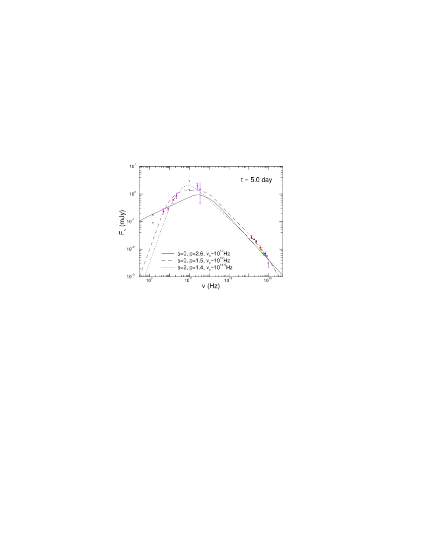
For 000301c, the measurements made around $t=4.3$ day span the widest frequency range. At the same time the optical emission exhibits a brightening. Figure 1 shows the afterglow spectrum at $t=5.0$ day, when the optical bump seems to have faded, obtained from the data closest to this time, using interpolations or extrapolations where necessary.

The radio spectrum of 000301c has a slope $\beta_{r}=-0.75\pm 0.15$ , between the values expected for optically thin ( $\beta_{r}=-1/3$ ) and thick ( $\beta_{r}=-2)$ emission, thus the absorption frequency $\nu_{a}$ must be around 10 GHz at 5 days.

Using the 250 GHz measurements reported by Berger et al. (2000) and the $K$ -band data of Rhoads & Fruchter (2001), we find that the millimeter–NIR spectral slope $\beta_{mK}$ is

\beta_{mK}=0.67\pm 0.04\quad{\rm at}\quad t=5\;{\rm d}\;.

(5)

Rhoads & Fruchter (2001) found that, after correction for Galactic extinction only, the spectral slope between the $K$ - and $R$ -bands is (see their Table 3)

\beta_{KR}=\left\{\begin{array}[]{ll}0.72\pm 0.04&t=2.1\;{\rm d}\\ 0.91\pm 0.04&t=3.0\;{\rm d}\\ 0.99\pm 0.15&t=5.0\;{\rm d}\\ 0.69\pm 0.10&t=7.6\;{\rm d}\end{array}\right.\;,

(6)

while at an earlier time, $t=1.8$ day, the $R-K$ color presented in their figure 2 gives $\beta_{KR}=0.47\pm 0.11$ . Rhoads & Fruchter (2001) find that, in order to reconcile the data with no evolution of $\beta_{KR}$ , a systematic error of 0.08 mag has to be added in quadrature to the $K$ and $R$ -band fluxes, and conclude that at least some of $K-R$ color evolution is real.

From spectroscopic observations, Feng et al. (2000) found that the optical spectral slope is $\beta_{O}\sim 1.1$ at $t=2$ day, while Jensen et al. (2001) arrived at

\beta_{O}=\left\{\begin{array}[]{ll}1.15\pm 0.26&t=4.0\;{\rm d}\\ 1.43\pm 0.28&t=5.0\;{\rm d}\end{array}\right.\;.

(7)

Equations (6) and (7) lead to

\beta_{O}-\beta_{KR}=\left\{\begin{array}[]{ll}0.23\pm 0.26&t\sim 4\;{\rm d}\\ 0.44\pm 0.32&t=5\;{\rm d}\end{array}\right.\;.

(8)

The above results provide only weak evidence for a curved (even after dereddening for Galactic extinction), softening afterglow spectrum. Jensen et al. (2001) and Rhoads & Fruchter (2001) attribute this departure from the power-law spectrum expected in the fireball model to extinction in the host galaxy. We note that softening of the NIR–optical spectrum, if real, suggests an intrinsic feature of the afterglow, as caused by a spectral break whose frequency decreases, passing through the optical domain. Given that the fastest possible decrease of the cooling frequency is $\nu_{c}\propto t^{-1/2}$ (see Panaitescu & Kumar 2001) and that the steepening $\Delta\beta=1/2$ of the spectrum across $\nu_{c}$ is smooth, it seems rather unlikely that the passage of $\nu_{c}$ would produce a detectable afterglow softening over a short timescale. This suggests that the evolving break is the $\nu_{*}$ associated with the high end of the electron distribution ( $\gamma_{*}$ ), which evolves as fast as $\nu_{i}$ and can be sharper than the $\nu_{c}$ -break.

It is also possible that the chromatic evolution of the afterglow between 2 and 5 days is caused by the same mechanism that yields the optical brightening seen at $\sim 3.5$ days. Most likely this excludes microlensing as the brightening mechanism, as lensing should not produce a chromatic afterglow behavior over less than a decade in frequency (note that, in general, microlensing of afterglows leaves chromatic signatures because the surface brightness profile of the source is wavelength-dependent).

3.2 Light-Curve Decay Indices

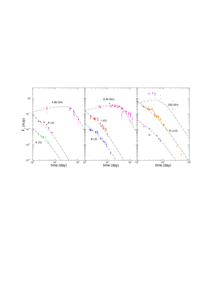
The 8.46 GHz radio emission of the 000301c afterglow, shown in Figure 2, exhibits a power-law decline with

\alpha_{r}=1.0\pm 0.2\quad{\rm at}\quad t\mathrel{\hbox to0.0pt{\raise 2.20013pt\hbox{$>$}\hss}{\lower 2.20013pt\hbox{$\sim$}}}30\;{\rm d}\;.

(9)

A steeper and highly uncertain decline, between $t^{-1}$ and $t^{-2.5}$ , is seen in the 4.86 GHz emission. Due to the curvature of the emitting surface, relativistic jets cannot produce significantly different decay indices at frequencies that are a factor of only two apart, so we presume that the light-curve indices at 4.86 GHz and 8.46 GHz are in fact the same and that the discrepancy can be resolved by interstellar scintillation.

The millimeter decay index at 250 GHz is not well determined by the data, nevertheless the $2\sigma$ upper limits shown in Figure 2 indicate that $\alpha_{m}>0.7$ . This shows that after few days the injection frequency $\nu_{i}$ is below $\sim 100$ GHz, unless the external medium is wind-like and the ordering of frequencies is $\nu_{a}<250\;{\rm GHz}<\nu_{c}<\nu_{i}$ , in which case it is analytically expected that $\alpha_{m}=2/3$ (Panaitescu & Kumar 2000), marginally consistent with the observations.

The NIR and optical emission of 000301c exhibited a break at few days. Using a smoothed dual power-law fit, Rhoads & Fruchter (2001) found a steepening from an asymptotic $\alpha_{K1}=0.09$ at early times to $\alpha_{K2}=2.26$ at late times, in the $K$ band, and from $\alpha_{R1}=0.69$ to $\alpha_{R2}=2.77$ in the $R$ band. Using a broken power-law approximation, Jensen et al. (2001) found $\alpha_{O1}=0.73\pm 0.27$ and $\alpha_{O2}=2.67\pm 0.51$ . At late times, when the effect of microlensing should be negligible, Garnavich et al. (2000b) found $\alpha_{O2}=2.9$ , close to the value reported by Sagar et al. (2000): $\alpha_{O2}=2.97\pm 0.04$ . With a more complex fitting function and without the last two $R$ magnitudes reported by Fruchter et al. (2000), which constrain the late time decay index, Bhargavi & Cowsik (2000) found $\alpha_{R1}=0.70\pm 0.07$ and $\alpha_{R2}=2.44\pm 0.29$ . Thus the asymptotic indices of the optical decay of 000301c are

\alpha_{R1}=0.70\pm 0.07\;,\quad\alpha_{R2}\geq 2.7\;,

(10)

implying that the decline of optical emission of this afterglow steepened by

\Delta\alpha_{R}=\alpha_{R2}-\alpha_{R1}\geq 1.9

(11)

over about one decade in observer time.

For a homogeneous external medium, the afterglow decay index is expected to increase by 3/4 when the jet edge becomes visible (i.e. the jet Lorentz factor drops below the inverse of its aperture, $\theta$ ), with an extra steepening of at most $p/4$ arising from the jet dynamics. It is thus hard to see how collimation of ejecta could account alone for the magnitude $\Delta\alpha_{R}$ of the optical break of 000301c, unless the afterglow decay before 3 days is significantly flattened by the brightening mechanism we see at 3–5 days, so that the observed decay index $\alpha_{R1}$ is smaller than that the afterglow would have if this mechanism were not present. Given that it takes more than two decades in time to a jet expanding into an $r^{-2}$ medium to yield about 90% of the full break magnitude (Kumar & Panaitescu 2000), the $\Delta\alpha_{R}$ above rules out a model with a wind-like medium and an afterglow steepening due only to collimated ejecta.

4 Models for the 000301c Afterglow

We start with a model where the high energy spectral break $\nu_{*}$ is well above the optical domain and the light-curve steepening is due solely to the collimation of ejecta. In this case the external medium must be homogeneous, so that the light-curve steepening at the time $t_{j}$ , when the jet edge becomes visible, is as fast as possible.

If the cooling frequency were below the NIR-optical domain, then $\beta_{KR}=p/2$ , thus the observed slope at 5 days (eq. [6]), after the optical brightening, would require $p=1.98\pm 0.30$ . Then the decay index of the optical emission at $t>t_{j}$ would approach asymptotically $\alpha_{R2}\sim p\mathrel{\hbox to0.0pt{\raise 2.20013pt\hbox{$<$}\hss}{\lower 2.20013pt\hbox{$\sim$}}}2.3$ , and would be shallower than observed (eq. [10]). Therefore the cooling frequency should be above the NIR–optical domain.

At few days, the injection frequency $\nu_{i}$ must be below the millimeter range, to explain the decay of the 250 GHz emission (§3.2, Figure 2). Then $\beta_{mK}=(p-1)/2$ and the observations at 5 days (eq. [5]) lead to $p=2.34\pm 0.08$ , which is still below $\alpha_{R2}$ . Therefore it may be difficult to reconcile within the jet model the spectrum and the late time optical decay of 000301c.

The best fit obtained with a jet model having the cooling frequency above optical and a homogeneous external medium is shown in Figure 2. Its $\chi^{2}=680$ for 132 degrees of freedom (df) is large in part because microlensing does not produce the brightening seen around 3.5 days, for reasons discussed below, the 28 NIR/optical measurements between 3.0 and 4.3 days yielding $\Delta\chi^{2}=210$ . To test the ability of only the jet model to account for the general features of 000301c, we eliminate the 3.0–4.3 days data and microlensing from the modeling. The new best fit has $\chi^{2}=480$ for 98 df (see Figure 2).

One reason for which the new $\chi^{2}$ is still large is that a relativistic jet yields the same $t^{-p}$ decay after $t_{j}$ at all frequencies above $\nu_{i}$ . However, in 000301, the late time decay indices of the 8.46 GHz and $R$ -band light-curves differ significantly. For the jet models shown in Figure 2, the 14 measurements made at 8.46 GHz after 30 days yield $\Delta\chi^{2}=68$ . Berger et al. (2000) explain this discrepancy (see their Figure 2) between the jet model and the radio emission of 000301c as the result of interstellar scintillation. Even if ISS were strong enough to accommodate the observations, the radio data should have been randomly scattered around the model light-curve, both having the same trend, which is unlike the behaviors illustrated in Figure 2.

The results of Figure 2 point to yet another reason for the large $\chi^{2}$ we obtain: the optical steepening of 000301c is too fast and too large to be explained with a jet break, as was expected based on analytical considerations (§3.2). For this reason we turn now to a “modified jet model”, where the passage through the optical of the $\nu_{*}$ break associated with the steepening of the electron distribution at $\gamma_{*}$ yields a light-curve steepening. As noted in §3.1, the passage of a spectral break is suggested by the softening of the NIR–optical spectrum (eq. [5]). The time and magnitude of the light-curve break caused by the $\nu_{*}$ -crossing depend on the location of $\gamma_{*}$ and on the steepening of the electron distribution at $\gamma_{*}$ , i.e. the parameters $\epsilon$ and $\delta p$ introduced in §2.1.

First note that, within the jet model, the quasi-constant 8.46 GHz emission prior to 30 days has two possible explanations:
$1)$ the ejecta are collimated, the jet edge becoming visible at few days, so that $F_{\nu}\propto t^{-1/3}$ before the passage of $\nu_{i}$ and $F_{\nu}\propto t^{-p}$ after that. These analytical results (Rhoads 1999) are not very accurate for moderately relativistic jets ( $\Gamma<10$ ), where we find numerically smaller decay indices. Nevertheless a hard electron distribution, with $p\mathrel{\hbox to0.0pt{\raise 2.20013pt\hbox{$<$}\hss}{\lower 2.20013pt\hbox{$\sim$}}}1.5$ , is required by the observed $\alpha_{r}\sim 1$ . Since the observed $\beta_{mK}$ (eq. [5]) is larger than $(p-1)/2$ , the cooling break must be below NIR. The external medium can be either homogeneous or wind-like.
$2)$ the external medium is a wind and the ejecta spherical, the radio emission evolving as $F_{\nu}\approx const$ before $\nu_{i}=\nu$ and as $F_{\nu}\propto t^{-(3p-1)/4}$ thereafter. The observed $\alpha_{r}$ (eq. [9]) requires that $p=1.7\pm 0.3$ . As in the first case, $\beta_{mK}>(p-1)/2$ implies that $\nu_{c}$ is below NIR. Given that the jet break is very smooth if the external medium is wind-like, this case is not readily distinguishable from a jet interacting with a wind.

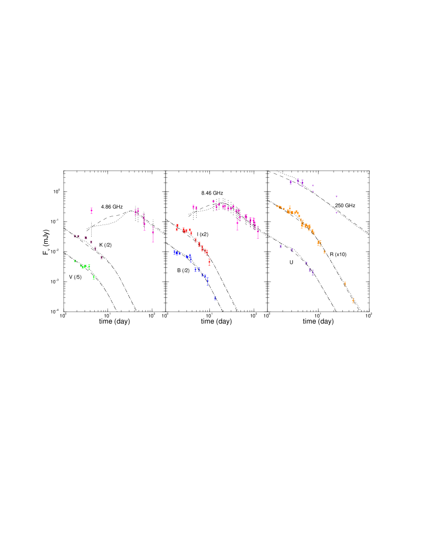
Figure 3 shows the best fits we obtain with a modified jet interacting with a homogeneous medium, with and without lensing and the 3.0–4.3 day data. In the latter case, the resulting fit has $\chi^{2}=120$ for 96 df, being marginally acceptable. Note that, in either case, the modified jet yields a significantly better fit than the ”traditional” jet model with $p>2$ and optical steepening caused by collimation. The best fits obtained with a modified jet and a wind-like medium are shown in Figure 4. Without microlensing and the 3.0–4.3 days data, it has $\chi^{2}=140$ for 96 df, being unacceptable. The light-curves shown in Figures 3 and 4 prove that, for either type of external medium, microlensing does not yield an afterglow brightening but only a flattening, for the reasons discussed below.

As found by many researchers (Waxman 1997, Panaitescu & Mészáros 1998, Sari 1998, Granot, Piran, & Sari 1999), at high frequencies, a spherical, relativistic fireball appears as a disk whose brightness surface increases toward the edge. An increasing magnification through lensing requires that the source is initially outside the Einstein disk. The peak magnification is obtained when, due to the source expansion (eqs. [1] and [2]), its edge crosses the Einstein disk. A significant magnification for a short duration (1–2 days for 000301c) constrains the size of the Einstein disk in two ways: it cannot be much smaller than the source size at the time of maximum lensing, as in this case the magnification would be weak, but it cannot be larger than it either, because the lensing event would last longer than the time when the maximum magnification is produced (3–4 days for 00301c). For the jet models with microlensing presented in Figure 2–4, the evolution of the source size and of the surface brightness distribution are such that the best fits are obtained if, at the time of maximum magnification ( $\sim 3.5$ days), the afterglow apparent size is twice larger than the Einstein disk. For this source–lens geometry, the source is too large for microlensing to yield a peaked light-curve.

Garnavich et al. (2000b) have obtained peaked lensed light-curves by approximating the source image with an annulus, whose fractional width (16%) was obtained by fitting the data. Granot & Loeb (2001) have calculated microlensed light-curves using the surface brightness distribution of a spherical, relativistic afterglow, and have found a peak magnification factor $\sim 2$ , supporting the microlensing model of Garnavich et al. (2000) for 000301c. We note, however, that in 000301c, the optical brightening occurs at times when jet effects are important, thus the source geometry and dynamics are not those expected for a spherical fireball. According to Ioka & Nakamura (2001), the surface brightness distribution of a spreading jet is rather uniform. We also note that, at the time of optical brightening, the jets of Figure 3 and 4 are not very relativistic ( $\Gamma\sim$ several), which makes the surface brightness distribution even more uniform. Therefore, in our modeling of 000301c, jet effects and the mildly relativistic motion of the source lead to an afterglow whose image at optical frequencies is not like the narrow ring envisaged by Garnavich et al. (2000b), but more like a disk.

5 Conclusions

The analysis presented in §4 shows that the “traditional” jet model cannot reconcile the late time decay indices of the 8.5 GHz and $R$ -band light-curves of 000301c, and cannot account for the magnitude of the steepening exhibited by decay of its optical emission. We attribute the latter to the passage of a spectral break $\nu_{*}$ associated with a steepening of the power-law electron distribution at high Lorentz factors. This also provides a natural explanation for the curvature of the optical spectrum observed by Jensen et al. (2001) without the help of host extinction, and for the possible softening of the NIR–optical spectrum implied by the results of Jensen et al. (2001) and Rhoads & Fruchter (2001), at about the same time when the steepening of the optical fall-off of 000301c occurred. Note that a chromatic evolution of the afterglow emission over less than a decade in frequency cannot be due to microlensing or to jet effects.

A break in the electron distribution was also used by Li & Chevalier (2001) to model the emission of 000301c in the framework of spherical ejecta interacting with a wind-like external medium, and by Panaitescu & Kumar (2001) for the afterglow of GRB 991216, where its was found that a jet model with a broken power-law injected electron distribution accommodates the data better than the simple jet model. Although the optical light-curve breaks shown in Figures 3 and 4 are mostly due to the $\nu_{*}$ -passage, the collimation of ejecta is still present in the model, to obtain consistency between the hard electron index $p\mathrel{\hbox to0.0pt{\raise 2.20013pt\hbox{$<$}\hss}{\lower 2.20013pt\hbox{$\sim$}}}1.5$ and the $t^{-1}$ late radio decay.

We find marginally acceptable fits only for a jet interacting with a homogeneous medium, and after excluding the 3.0–4.3 days data, as we could not model the brightening of 000301c during this time using microlensing. From the variation of $\chi^{2}$ around its minimum, we arrive at the following 95% confidence level intervals for a single parameter:

E_{0}=(1.8-3.6)\times 10^{50}\;{\rm erg}\;,\quad\theta_{0}=10.8-14.6\;{\rm deg}\;,

n=13-38\;{\rm cm^{-3}}\;,\quad\varepsilon_{B}=0.032-0.15\;,

\varepsilon_{e}=0.030-0.065\;,\quad p=1.41-1.59\;,

\epsilon=0.34-0.54\;,\quad\delta p=0.9-1.3\;.

These results are given only to show the statistical uncertainties of the model parameters, and should not be considered absolute limits. For such limits one would need to know the “model error bars”, which may be larger than the above uncertainties.

Consistency between the expected decay of jet light-curves and that seen in 000301c at 8.5 GHz after 30 days requires a hard electron distribution, with $p\mathrel{\hbox to0.0pt{\raise 2.20013pt\hbox{$<$}\hss}{\lower 2.20013pt\hbox{$\sim$}}}1.6$ , similar to the indices obtained by Malkov (1999) for Fermi acceleration in the limit when particles acquire a significant fraction of the shock energy, and by Ellison, Jones, & Reynolds (1990) and Baring (2000) for particle diffusion driven by large angle scatterings.

We note that the time when the afterglow steepening is seen constrains the $\nu_{*}$ break frequency and determines the electron fractional energy $\epsilon$ . In light of this, is interesting to note that for 000301c we find an electron fractional energy close to equipartition, providing thus a natural reason for steepening of the electron distribution at high energies.

The model lensed light-curves we obtain show that microlensing by can yield a significant magnification but does not provide a good fit to the observations, failing to produce a peak at maximum lensing. The reason is that the afterglow surface brightness is not sufficiently concentrated toward the edge of the visible disk to yield a light-curve peak when this edge crosses the Einstein disk of the lens. We emphasize that this conclusion is subject to the correctness of the assumptions made in our treatment of the jet model.

Evidently, we do not rule out microlensing of 000301c within the framework of other afterglow models (e.g. non-uniform jets). An inhomogeneity in the external medium or a pile-up of electrons (Protheroe & Stanev 1999) at the $\gamma_{*}$ break, above which electrons are inefficiently accelerated, could in principle explain the brightening that preceded the steepening of the optical emission of 000301c.

It is a pleasure to thank Pawan Kumar (IAS) for useful suggestions and comments on this work

REFERENCES

Baring, M. 2000, 26th International Cosmic Ray Conference, vol IV, p5, eds. B. Dingus, D. Kieda, and M. Salamon, AIP Conf. Proc. 516, New York : AIP Press

Berger, E. et al. 2000, ApJ, 545, 56

Bernabei, S. et al. 2000, GCN^∗ 599

Bhargavi, S. & Cowsik, R. 2000, ApJ, 545, L77

Campins, H., Rieke, G., & Lebofsky, M. 1985, AJ, 90, no 5, 896

Castro, S. et al. 2000, GCN^∗ 605

Ellison, D., Jones, F., & Reynolds, S. 1990, ApJ, 360, 702

Feng, M. et al. 2000, GCN^∗ 607

Fruchter, A. et al. 2000, GCN^∗ 627, 701

Fukugita, M., Shimasaku, K., & Ichikawa, T. 1995, PASP, 107, 945

Gal-Yam, A. et al. 2000, GCN^∗ 593

Garnavich, P. et al. 2000a, GCN^∗ 573, 581

Garnavich, P., Loeb, A., & Stanek, K. 2000b, ApJ, 544, L11

Goodman, J. 1997, New Astronomy, 2, 49

Granot, J., Piran, T., & Sari, R. 1999, ApJ, 513, 679

Granot, J. & Loeb, A. 2001, ApJL, submitted (astro-ph/0101234)

Halpern, J. et al. 2000, GCN^∗ 578, 604

Ioka, K. & Nakamura, T. 2001, ApJ, submitted (astro-ph/0102028)

Jensen, B. et al. 2001, A&A, submitted (astro-ph/0005609)

Kobayashi, N. et al. 2000, GCN^∗ 587

Kumar, P. & Panaitescu, A. 2000, ApJ, 541, L9

Li, Z., Chevalier, R. 2001, ApJ, submitted (astro-ph/0010288)

Loeb, A, & Perna, R. 1998, ApJ, 495, 597

Malkov, M. 1999, ApJ, 511, L53

Masetti, N. et al. 2000, A&A, 359, L23

Mujica, R. et al. 2000, GCN^∗ 597

Mészáros, P. & Rees, M.J. 1997, ApJ, 476, 232

Mészáros, P., Rees, M.J., & Wijers, R. 1999, MNRAS, 306, L39

Panaitescu, A. & Kumar, P. 2000, ApJ, 543, 66

Panaitescu, A. & Kumar, P. 2001, ApJ, 554, in press (astro-ph/0010257)

Panaitescu, A. & Mészáros, P. 1998, ApJ, 493, L31

Protheroe, R. & Stanev, T. 1999, APh, 10, 185

Rhoads, J. 1999, ApJ, 525, 737

Rhoads, J. & Fruchter, A. 2001, ApJ, 546, 117

Sagar, R., Mohan, V., Pandey, S., & Castro-Tirado, A. 2000, BASI, 28, 499

Sari, R., Piran, T. & Narayan, R. 1998, ApJ, 497, L17

Sari, R. 1998, ApJ, 494, L49

Smette, A. et al. 2001, ApJ, submitted (astro-ph/0007202)

Veillet, C. & Boer, M. 2000, GCN^∗ 588, 598, 610, 611

Walker, M. 1998, MNRAS, 294, 307

Waxman, E. 1997, ApJ, 491, L19

^∗ GCN Circulars can be found at http://gcn.gsfc.nasa.gov/gcn/

Refer to caption — Fig. 1.—: Spectrum of the 000301c afterglow at $t=5.0$ day constructed from the measurements closest to this epoch and linear interpolations at low frequencies or using the fit of Rhoads & Fruchter (2001) in the NIR-optical. Optical fluxes are corrected for Galactic extinction of $E(B-V)=0.053$ . Downward triangles indicate $1\sigma$ and $2\sigma$ upper limits (note that Berger et al. 2000 report a flux of $2.85\pm 0.95$ mJy at 100 GHz an 4.26 days; the upper limits shown here are their measurement at 5.09 days). The low flux at $10^{15}$ Hz, representing the $UV$ measurement of Smette et al. (2001), could be due to intergalactic $Ly\alpha$ absorption. The solid, dashed and dotted lines represents the spectra obtained with the jet models described in Figures 2, 3, and 4, respectively.