A Search for OH Megamasers at $z>0.1$.   II.  Further Results

Abstract

We present current results of an ongoing survey for OH megamasers in luminous infrared galaxies at the Arecibo Observatory. The survey is now two-thirds complete, and has resulted in the discovery of 35 new OH megamasers at $z>0.1$, 24 of which are presented in this paper. We discuss the properties of each source in detail, including an exhaustive survey of the literature. We also place upper limits on the OH emission from 107 nondetections and list their IR, radio, and optical properties. The survey detection rate is 1 OH megamaser for every 6 candidates overall, but is a strong function of the far IR luminosity of candidates and may depend on merger stage or on the central engine responsible for the IR luminosity in the merging galaxy pair. We also report the detection of IRAS 12032+1707, a new OH gigamaser.

1 Introduction

The first paper in this series presents the motivation, goals, and preliminary results of a survey for OH megamasers (hereafter OHMs) at the Arecibo Observatory (Darling & Giovanelli 2000; hereafter Paper I). To recap the survey, we use the Point Source Catalog redshift survey (PSCz; Saunders et al. 2000) to select OHM candidates which lie within the Arecibo declination range $0^{\circ}<\delta<37^{\circ}$ and have $z>0.1$. The requirement for candidates to have a measured redshift $z>0.1$ and an IRAS detection at 60 $\mu$m guarantees that they are (ultra)luminous IR galaxies ([U]LIRGs). The survey is designed to double the sample of OHMs to roughly 100, and increase the $z>0.1$ sample by a factor of seven. The Arecibo OHM survey will provide a uniform flux-limited sample which can be tied to the low-redshift FIR luminosity function (see Paper I). One can subsequently perform deep searches for OH line emission at various redshifts and effectively measure the evolution of the FIR luminosity function with redshift. Since ULIRGs are major mergers (Clements et al., 1996), one can also measure the number evolution of galaxies by measuring the number density of OHMs at various redshifts (Briggs, 1998). A measure of the number density evolution of galaxies breaks the degeneracy between luminosity evolution and number density evolution seen in the luminosity function evolution derived from redshift surveys (eg - Le Févre et al. 2000; Lilly et al. 1995; Ellis et al. 1996) and provides strong constraints on hierarchical models of galaxy formation and evolution (eg - Abraham 1999; Governato 1999). The OHM sample will also provide new perspective on OH megamaser environments, lifetimes, engines, and structure. The $z>0.1$ sample is distant enough that many masing regions will have sufficiently small angular scales to show interstellar scintillation (Walker, 1998). Indeed, several OHMs have been observed to vary in time, and a comprehensive study of OHM variability is underway. Many of the OHM hosts have optical spectral classification of their nuclei available in the literature, but those which do not are under investigation at the Palomar 5m telescope. Finally, as in any survey, the Arecibo OHM survey is likely to produce unexpected results or detections which cannot be predicted a priori. Several of the new detections in this paper and Paper I have unexpected properties (see §3.2), and more surprises are likely before the survey is complete.

This paper is primarily dedicated to releasing the new OH megamaser detections for rapid community access. Paper I presented 11 OHMs, one OH absorber, and 53 nondetections, accounting for $22\%$ of the survey. This paper presents 24 new OHMs and 107 nondetections, accounting for $44\%$ of the total survey. We discuss the observations, data reduction, and newly implemented RFI mitigation techniques in Section 2, the new detections as well as the non-detections in Section 3, and the results to date and the plan for the remainder of the survey in Section 4.

This paper parameterizes the Hubble constant as $H_{\circ}=75\ h_{75}$ km s^-1 Mpc^-1, assumes $q_{\circ}=0$, and uses $D_{L}=(v_{CMB}/H_{\circ})(1+0.5z_{CMB})$ to compute luminosity distances from $v_{CMB}$, the radial velocity of the source in the cosmic microwave background (CMB) rest-frame. Line luminosities are always computed under the assumption of isotropic emission.

2 Observations and Data Reduction

Observations at Arecibo with the L-band receiver were performed in an identical manner to earlier survey work by nodding on- and off-source, each for a 4-minute total integration, followed by firing a noise diode (see Paper I). Spectra were recorded in 1-second intervals (a significantly faster dump rate than usual for spectroscopy work at Arecibo) to facilitate radio frequency interference (RFI) flagging and excision in the time-frequency domain. Data was recorded with 9-level sampling in 2 polarizations of 1024 channels each, spanning a 25 MHz bandpass centered on redshifted 1666.3804 MHz (the mean of the 1667.359 and 1665.4018 MHz OH lines).

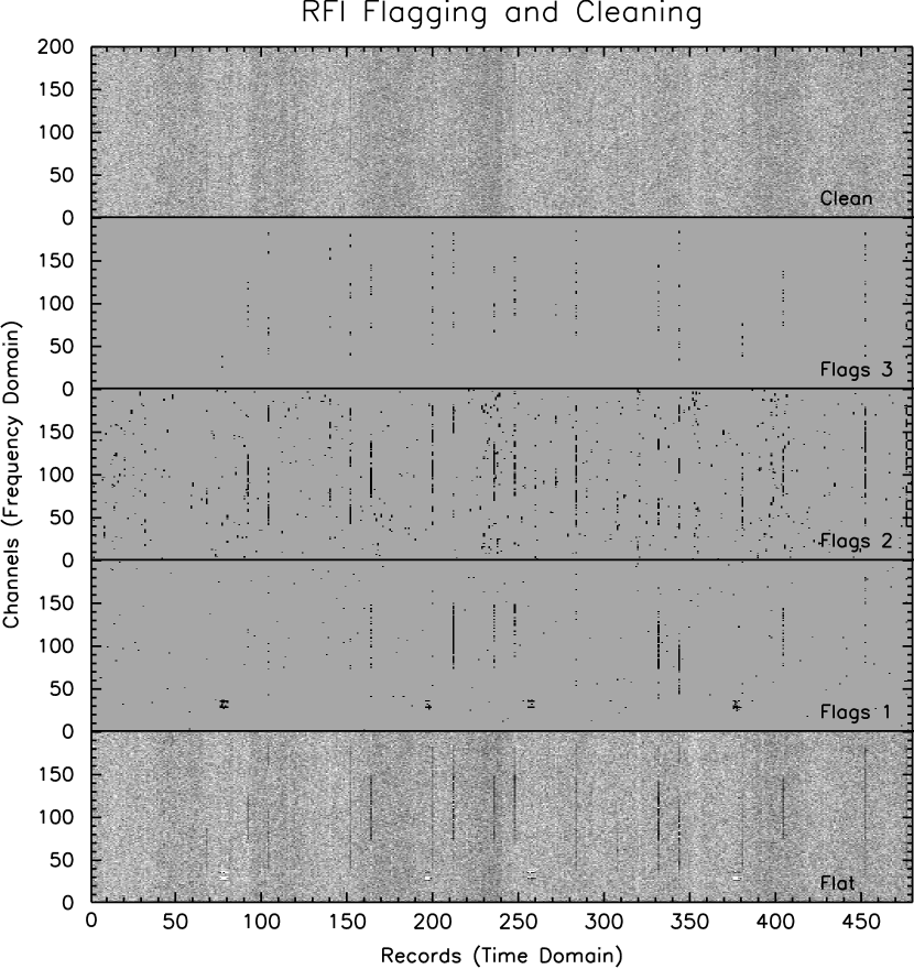
Figure 1: Frequency-time slices of an unusually dense radio frequency interference (RFI) environment showing several stages of the RFI flagging and cleaning procedure. Each channel spans 24.4 kHz, and a 200 channel slice is shown in the frequency domain. The horizontal scale represents a time series of 1 second records; the first 240 records are the on-source position and the last 240 records are the off-source position. Panels from bottom to top illustrate: a flattened “dirty” image in which the rate of occurrence and the spectral extent of RFI is emphasized by the dark pixels (Flat); the flags array produced in the first time-domain filter (Flags 1); the flags array produced in the second time-domain filter after spectral boxcar averaging (Flags 2); the flags array produced from near neighbors (Flags 3); and the final cleaned image (Clean). The greyscale is normalized such that the median grey color (such as seen in the background of the Flags panels) represents zero, dark pixels are positive values, and light pixels are negative. Flagged channels in the Flags arrays are set to unity (black), whereas flagged channels in the cleaned image are set to zero (they are not in fact included in the final time averaged spectrum).

All data reduction and analysis was performed with the AIPS++ software package using home-grown routines for single dish reduction. We included in the reduction pipeline RFI flagging routines designed to identify two types of RFI observed at Arecibo: strong features more than $3\sigma$ above the time-domain noise and spectrally broad, low-level RFI which is time-variable. Figure 1 illustrates with time-frequency array images some of the RFI flagging steps outlined below. The reduction pipeline and RFI flagging procedure follow the steps: (1) form an array in time and frequency from a 4-minute on-off pair (1024 channels $\times$ 480 1-second records); (2) flatten the array “image” by subtracting the time-averaged or median (both are examined) bandpass shape (average/median of 240 records; see Figure 1, Flat); (3) compute an RMS noise spectrum (RMS across the time domain) and fit this spectrum with a high-order polynomial; (4) compare the smooth polynomial noise spectrum to individual records and flag $3\sigma$ channels (Flags 1 in Figure 1); (5) perform a boxcar spectral average over 5 channels for each record and repeat the RMS noise spectrum fitting and channel flagging (Flags 2 in Figure 1); (6) flag channels which have at least 8 flagged neighbors in a 10 channel box in the spectral regime (Flags 3 in Figure 1); (7) set all flagged channels to zero in the flattened data to obtain a clean image (Clean in Figure 1); (8) form an average on- and off-source spectrum from the original raw data, rejecting flagged channels and keeping track of the number of records averaged in each channel; (9) perform the usual (on$-$off)/off conversion to obtain an intensity scale expressed as a percentage of the system temperature, and use VLA calibrators and noise diodes to convert to flux density units (mJy); (10) average multiple on-off pairs and polarizations weighted by the number of records used in each channel, keeping track of the effective noise present in each channel; (11) fit and subtract baselines and hanning smooth to obtain the final spectra. The frequency resolution after hanning smoothing is 49 kHz (10 km s^-1 at $z=0.1$), and the uncertainty in the absolute flux scale is $8\%$. The RFI flagging procedure was tested on both synthetic and real data with the result that time-constant signals are unaffected by the process to within roundoff errors introduced in the processing, and that a reliable estimate of the weight, or effective integration time, on a single channel is the total number of records used in forming the time average, excluding flagged records. Each spectral channel in a calibrated time-averaged spectrum may have a different effective integration time and hence a different effective intrinsic radiometer noise level. We include a normalized weights spectrum with each OHM spectrum in Figure 2. Depressions in the weights spectra indicate the presence of RFI, which may or may not have been completely flagged and removed from the final spectra. Spectral channels with low weights should thus be treated with skepticism.

The techniques described here were not performed on the data presented in Paper I. We applied these data reduction steps to several of the Paper I spectra and compared the results to the published spectra. Spectra are not significantly changed except in cases of significant RFI (the usual averaging process tends to mitigate low-level RFI anyway), although the ANALYZ reduction process used for the Paper I spectra tends to produce lower overall RMS noise levels. We attribute this to the automatic application of hanning smoothing to each 6-second record in ANALYZ, rather than applying hanning smoothing to the final spectrum as we do in AIPS++. Electronic versions of all spectra processed following the methods described in this paper, for the sources in both papers, are available upon request.

3 Results

3.1 Nondetections

Tables A Search for OH Megamasers at $z>0.1$.   II.  Further Results and A Search for OH Megamasers at $z>0.1$.   II.  Further Results list respectively the optical/FIR and radio properties of 107 OH non-detections. Note that IRAS 03477+2611 also appears in Paper I; reobservation produced a stronger OH flux limit on this candidate, as listed in Table A Search for OH Megamasers at $z>0.1$.   II.  Further Results of this paper. Table A Search for OH Megamasers at $z>0.1$.   II.  Further Results lists the optical redshifts and FIR properties of the non-detections in the following format. Column (1): IRAS Faint Source Catalog (FSC) name. Columns (2) and (3): Source coordinates (epoch B1950.0) from the FSC, or the Point Source Catalog (PSC) if unavailable in the FSC. Columns (4), (5) and (6): Heliocentric optical redshift, reference, and corresponding velocity. Uncertainties in velocities are listed whenever they are available. Column (7): Cosmic microwave background rest-frame velocity. This is computed from the heliocentric velocity using the solar motion with respect to the CMB measured by Lineweaver et al. (1996): $v_{\odot}=368.7\pm 2.5$ km s^-1 towards $(l,b)=(264\fdg 31\pm 0\fdg 16,48\fdg 05\pm 0\fdg 09)$. Column (8): Luminosity distance computed from $v_{CMB}$ via $D_{L}=(v_{CMB}/H_{\circ})(1+0.5z_{CMB})$, assuming $q_{\circ}=0$. Columns (9) and (10): IRAS 60 and 100 $\mu$m flux densities in Jy. FSC flux densities are listed whenever they are available. Otherwise, PSC flux densities are used. Uncertainties refer to the last digits of each measure, and upper limits on 100 $\mu$m flux densities are indicated by a “less-than” symbol. Column (11): The logarithm of the far-infrared luminosity in units of $h_{75}^{-2}L_{\odot}$. $L_{FIR}$ is computed following the prescription of Fullmer & Lonsdale (1989): $L_{FIR}$ $=3.96\times 10^{5}D_{L}^{2}(2.58f_{60}+f_{100})$, where $f_{60}$ and $f_{100}$ are the 60 and 100 $\mu$m flux densities expressed in Jy, $D_{L}$ is in $h_{75}^{-1}$Mpc, and $L_{FIR}$ is in units of $h_{75}^{-2}L_{\odot}$. If $f_{100}$ is only available as an upper limit, the permitted range of $L_{FIR}$ is listed. The lower bound on $L_{FIR}$ is computed for $f_{100}=0$ mJy, and the upper bound is computed with $f_{100}$ set equal to its upper limit. The uncertainties in $D_{L}$ and in the IRAS flux densities typically produce an uncertainty in $\log L_{FIR}$ of $0.03$.

Table A Search for OH Megamasers at $z>0.1$.   II.  Further Results lists the 1.4 GHz flux density and the limits on OH emission of the non-detections in the following format: Column (1): IRAS FSC name, as in Table A Search for OH Megamasers at $z>0.1$.   II.  Further Results. Column (2): Heliocentric optical redshift, as in Table A Search for OH Megamasers at $z>0.1$.   II.  Further Results. Column (3): $\log$ $L_{FIR}$ , as in Table A Search for OH Megamasers at $z>0.1$.   II.  Further Results. Column (4): Predicted isotropic OH line luminosity, $\log L_{OH}^{pred}$, based on the Malmquist bias-corrected $L_{OH}$-$L_{FIR}$ relation determined by Kandalian (1996) for 49 OHMs: $\log L_{OH}=(1.38\pm 0.14)\log L_{FIR}-(14.02\pm 1.66)$ (see Paper I). Column (5): Upper limit on the isotropic OH line luminosity, $\log L_{OH}^{max}$. The upper limits on $L_{OH}$ are computed from the RMS noise of the non-detection spectrum assuming a “boxcar” line profile of rest frame width $\Delta v=150$ km s^-1 and height 1.5 $\sigma$: $\log L_{OH}^{max}=\log(4\pi D_{L}^{2}\ 1.5\sigma[\Delta v/c][\nu_{\circ}/(1+z)])$. The assumed rest frame width $\Delta v=150$ km s^-1 is the average FWHM of the 1667 MHz line of the known OHM sample. Column (6): On-source integration time, in minutes. Column (7): RMS noise values in flat regions of the non-detection baselines, in mJy, after spectra were hanning smoothed to a spectral resolution of 49 kHz. Column (8): 1.4 GHz continuum fluxes, from the NRAO VLA Sky Survey (NVSS; Condon et al. 1998). If no continuum source lies within 30$\arcsec$ of the IRAS coordinates, an upper limit of 5.0 mJy is listed. Column (9): Optical spectroscopic classification, if available. Codes used are: “S2” = Seyfert type 2; “S1” = Seyfert type 1; “A” = active nucleus; “C” = composite active and starburst nucleus; “H” = H II region (starburst); and “L” = low-ionization emission region (LINER). References for the classifications are listed in parentheses and included at the bottom of the Table. Column (10): Source notes, listed at the bottom of the Table.

We can predict the expected isotropic OH line luminosity, $L_{OH}^{pred}$, for the OHM candidates based on the $L_{OH}$-$L_{FIR}$ relation determined by Kandalian (1996; see Paper I) and compare this figure to upper limits on the OH emission derived from observations, $L_{OH}^{max}$, for a rough measure of the confidence of the non-detections. Note, however, that the scatter in the $L_{OH}$–$L_{FIR}$ relation is quite large: roughly half an order of magnitude in $L_{FIR}$ and one order of magnitude in $L_{OH}$ (see Kandalian 1996). Among the non-detections, 18 out of 107 galaxies have $L_{OH}^{pred}<L_{OH}^{max}$, indicating that longer integration times are needed to unambiguously confirm these non-detections, and 13 out of 107 candidates have $L_{OH}^{max}$ within the range of $L_{OH}^{pred}$ set by an upper limit on $f_{100}$. Integration times were a compromise between efficient use of telescope time and the requirement for a meaningful upper limit on $L_{OH}$ for non-detections. Given the scatter of identified OHMs about the $L_{OH}$–$L_{FIR}$ relation, we estimate that there are less than 8 additional OHMs among the non-detections, but this estimate relies on uncertain statistics of small numbers. A thorough analysis of completeness will be performed once the survey is complete.

3.2 New OH Megamaser Detections

Tables A Search for OH Megamasers at $z>0.1$.   II.  Further Results and 4 list respectively the optical/FIR and radio properties of the 24 new OHM detections. Spectra of the 24 OHMs appear in Figure 2. The column headings of Table A Search for OH Megamasers at $z>0.1$.   II.  Further Results are identical to those of Table A Search for OH Megamasers at $z>0.1$.   II.  Further Results. Table 4 lists the OH emission properties and 1.4 GHz flux density of the OH detections in the following format. Column (1): IRAS FSC name. Column (2): Measured heliocentric velocity of the 1667.359 MHz line, defined by the center of the FWHM of the line. The uncertainty in the velocity of the line center is estimated assuming an uncertainty of $\pm 1$ channel ($\pm 49$ kHz) on each side of the line. Column (3): On-source integration time in minutes. Column (4): Peak flux density of the 1667 MHz OH line in mJy. Column (5): Equivalent width-like measure in MHz. $W_{1667}$ is the ratio of the integrated 1667 MHz line flux to its peak flux. Ranges are listed for $W_{1667}$ in cases where the identification of the 1665 MHz line is unclear. Column (6): Observed FWHM of the 1667 MHz OH line in MHz. Column (7): Rest frame FWHM of the 1667 MHz OH line in km s^-1. The rest frame width was calculated from the observed width as $\Delta v_{rest}=c(1+z)(\Delta\nu_{obs}/\nu_{\circ})$. Column (8): Hyperfine ratio, defined by $R_{H}=F_{1667}/F_{1665}$, where $F_{\nu}$ is the integrated flux density across the emission line centered on $\nu$. $R_{H}=1.8$ in thermodynamic equilibrium, and increases as the degree of saturation of masing regions increases. In many cases, the 1665 MHz OH line is not apparent, or is blended into the 1667 MHz OH line, and a good measure of $R_{H}$ becomes difficult without a model for the line profile. It is also not clear that the two lines should have similar profiles, particularly if the lines are aggregates of many emission regions in different saturation states. Some spectra allow a lower limit to be placed on $R_{H}$, indicated by a “greater than” symbol. Blended or noisy lines have uncertain values of $R_{H}$, and are indicated by a tilde, but in some cases, separation of the two OH lines is impossible and no value is listed for $R_{H}$. Column (9): Logarithm of the FIR luminosity, as in Table A Search for OH Megamasers at $z>0.1$.   II.  Further Results. Column (10): Predicted OH luminosity, $\log L_{OH}^{pred}$, as in Table A Search for OH Megamasers at $z>0.1$.   II.  Further Results. Column (11): Logarithm of the measured isotropic OH line luminosity, which includes the integrated flux density of both the 1667.359 and the 1665.4018 MHz lines. Note that $L_{OH}^{pred}$ is generally less than the actual $L_{OH}$ detected (23 out of 24 detections). Column (12): 1.4 GHz continuum fluxes, from the NVSS. If no continuum source lies within 30$\arcsec$ of the IRAS coordinates, an upper limit of 5.0 mJy is listed.

The spectra of the OH detections are presented in Figure 2. The abscissae and inset redshifts refer to the optical heliocentric velocity, and the arrows indicate the expected velocity of the 1667.359 (left) and 1665.4018 (right) MHz lines based on the optical redshift, with error bars indicating the uncertainty in the redshift. The spectra refer to 1667.359 MHz as the rest frequency for the velocity scale. Spectra have had the dotted baselines subtracted, and the baselines have been shifted in absolute flux density such that the central channel has value zero. The small frame below each spectrum shows a weights spectrum, indicating the fractional number of records used to form the final spectrum after the RFI rejection procedure (§2). Channels with weights close to unity are “good” channels, whereas channels with lower than average weight are influenced by time-variable RFI and are thus suspect. The weights spectra are presented to indicate confidence in various spectral features, but note that often the RFI rejection procedure does a good job of cleaning channels and that channels with $\sim 10\%$ rejected records may be completely reliable (this is, after all, the point of the RFI cleaning procedure).

In order to quantitatively identify dubious 1665 MHz OH line detections, we compute the autocorrelation function (ACF) of each spectrum and locate the secondary peak (the primary peak corresponds to zero offset, or perfect correlation). Any correspondence of features between the two main OH lines will enhance the second autocorrelation peak and allow us to unambiguously identify 1665 MHz lines based not strictly on spectral location and peak flux, but on line shape as well. The secondary peak in the ACF of each spectrum, when present, is indicated by a small solid line over the spectra in Figure 2. We expect the offset of the secondary peak to be equal to the separation of the two main OH lines, properly redshifted: (1.9572 MHz)$/(1+z)$. The expected location of the secondary ACF peak is indicated in Figure 2 by a small dashed line over each spectrum. Both the expected and actual secondary peak positions are plotted offset with respect to the center of the 1667 MHz line, as defined by the center of the FWHM, rather than the peak flux.

We examined the Digitized Sky Survey (DSS) images of each new OH detection. The OHM hosts are generally faint, unresolved, and unremarkable in the DSS unless otherwise noted in the discussion of individual sources below. We also performed an exhaustive literature search for each new OHM, and searched the Hubble Space Telescope (HST) archives for fields containing OHM hosts. All relevant data are included in the discussions below. The weights spectra are generally clean across the OH line profiles, unless specifically noted. We make some observations and measurements specific to individual OH detections as follows.

04121+0223: The optical redshift and observed line velocities are in good agreement for this source. The predicted location of the 1665 MHz line from the 1667 MHz centroid and from the strong second peak in the spectral ACF are in good agreement and correspond to a significant spectral feature (a $2\sigma$ feature in single-channel flux density, but it is broad, with an integrated flux density of of 0.61 mJy MHz and FWHM of 1.54 MHz). There are clearly two distinct emission features in the 1667 MHz line: one fairly broad ($135\pm 12$ km s^-1 rest-frame FWHM) and one narrow ($37\pm 12$ km s^-1). The DSS image of IRAS 04121+0223 shows a slightly extended host galaxy.

07163+0817: The 1667 MHz line of this source shows an extremely narrow emission spike which appears to be spectrally unresolved ($24\pm 12$ km s^-1 rest-frame FWHM). The two 1667 MHz emission peaks may correspond to a toroidal emission configuration or to two masing nuclei in the merger. We use the centroid of the main 1667 MHz line complex (excluding the narrow emission spike) as the reference for the ACF and the predicted offset of the 1665 MHz line. The ACF is dominated by peaks produced when the strong OH emission spike corresponds with any other narrow spike in the spectrum. The predicted 1665 MHz line velocity seems to correspond roughly with a $3\sigma$ spectral feature. Assuming that this feature is the 1665 MHz line, we obtain $R_{H}\sim 5.5$. The identification of the 1665 MHz line is uncertain, which is indicated by the tilde in Table A Search for OH Megamasers at $z>0.1$.   II.  Further Results. The weights spectrum indicates some narrow RFI at 33500 km s^-1 which may mildly influence the integrated 1667 MHz line flux.

07572+0533: The ACF and offset predictions for the 1665 MHz line velocity show good agreement, but there is no significant corresponding spectral feature in this OH spectrum. We compute a lower limit on the hyperfine ratio assuming a square profile of width equal to the 1667 MHz line width and height $1\sigma$ to obtain $R_{H}\geq 10.4$. There appears to be a second OH line (a $3\sigma$ detection) offset blueward by 400 km s^-1 in the rest frame from the center of the main 1667 MHz line. This line is included in the computation of the isotropic OH line luminosity for this source. The features at 57300, 58150, and 58600 km s^-1 are identified with RFI. The weights array is otherwise clean across the OH spectrum.

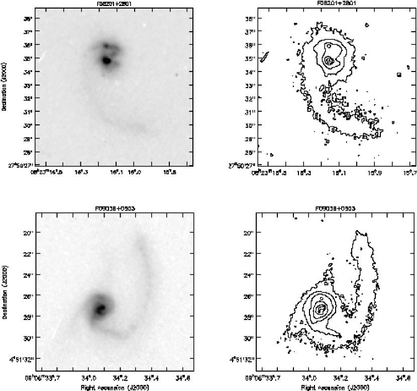
Figure 6: HST WFPC2 archive images of IRAS 08201+2801 and IRAS 09039+0503 (800 s exposures; F814W filter; $\lambda=7940$Å, $\Delta\lambda=1531$Å) reveal morphological signatures of interacting galaxies. The greyscale is linear, and contours are incremented by factors of 2. IRAS 08021+2801 shows two nuclei and an extended tidal tail. IRAS 09039+0503 has a double nucleus and three tidal tails.

08201+2801: The nucleus of this ULIRG was classified by Kim, Veilleux, & Sanders (1998) as a starburst. The spectrum around 52200 km s^-1 has been masked to remove incompletely subtracted strong Galactic H I emission. The ACF shows no second peak, but the predicted velocity of the 1665 MHz line corresponds to a feature of similar width to the main 1667 MHz line. There is a similar shoulder, however, on the blue side of the main line, which may indicate that the feature we identify as the 1665 MHz line is instead part of a high-velocity complex of low-level 1667 MHz emission. If we assume that the feature on the red side is the 1665 MHz line, then we obtain a lower bound on the hyperfine ratio: $R_{H}\geq 8.2$. Note that there is a mild depression in the weights spectrum near the expected 1665 MHz line, but we are satisfied that the RFI was successfully removed. The spectrum shows an absorption feature redward of the OH emission complex (the NVSS 1.4 GHz continuum flux of this source is 16.7 mJy; see Condon et al. 1998) which may indicate infall of molecular gas. This would be consistent with the picture of ULIRGs as merging systems in which gas and dust becomes concentrated into the merging nuclei by tidal angular momentum loss and subsequent infall. If the line is absorption in 1667 MHz, then the absorption minimum has a rest frame offset from the 1667 MHz emission line center of 750 km s^-1. If the line is absorption in 1665 MHz, the offset from the 1665 MHz emission line is 380 km s^-1. Alternatively, the absorption could occur in a physically distinct region from the masing region, along a different line of sight, such as in another nucleus. A WFPC2 HST archive image (F814W, 800 s) shows interesting morphology, with two nuclei connected by arcs, and a single kinked tidal tail (see Fig. 6). This is clearly an advanced merger, and we can measure a separation between the two nuclei for an indication of merger stage. The nuclear separation is 1.09″, corresponding to a projected distance of 2.83 kpc ($R=(1+z)^{-2}D_{L}\Delta\theta$). If the absorption feature at 51075 km s^-1 is associated with one of the two nuclei, while the emission is associated with the other nucleus, then we estimate a rough enclosed mass of $M(r)\simeq v^{2}R/G=3.7\times 10^{11}$ M_⊙ and a naive crossing time of $t_{cross}\simeq R/v=3.7\times 10^{6}$ years.

08279+0956: There is good agreement in this source between the OH line velocities, the optical redshift predictions for the two OH lines, the predicted location of the 1665 MHz line from the ACF, and the predicted location of the 1665 MHz line from the 1667 MHz line center. The isotropic OH line luminosity of this source is nearly an order of magnitude larger than we predict from $L_{FIR}$ . The weights spectrum is clean across the OH lines. The “absorption” feature at 61200 km s^-1 is produced by a resonance in the wide L-band feed at Arecibo.

08449+2332: No significant spectral feature corresponds to the predicted velocity of the 1665 MHz line from the 1667 MHz line centroid or from the ACF second peak. The emission profile shows a narrow line atop a broader base of emission, spanning 760 km s^-1 at $10\%$ of the peak flux density in the rest frame. Although the isotropic OH luminosity is somewhat low, it is still higher than the value predicted from $L_{FIR}$. A lower bound is calculated for the hyperfine ratio: $R_{H}\geq F_{1667}/(1\sigma\Delta\nu_{1667})=11.0$. The weights array is fairly clean across the OH line complex.

08474+1813: This source shows a broad 1667 MHz emission line which may be blended with the 1665 MHz line. The ACF has no secondary peak, but the optical redshift and the center of the 1667 MHz line both indicate a 1665 MHz line velocity corresponding to the blended feature redward of the bulk of the emission. Using the assumption that this is the 1665 MHz line as a lower limit, $R_{H}\geq 3.0$. The equivalent width-like measure, $W_{1667}$, is assigned a range of values which bracket the limiting cases for the presence of the 1665 MHz line. The weights spectrum shows a mild dip near the possible 1665 MHz line, indicating that the 1665 MHz line identification and measurements should be interpreted with caution.

09039+0503: The nucleus of this OHM host is classified by Veilleux, Kim, & Sanders (1999) as a LINER. The ACF and 1667 MHz line center predictions are in excellent agreement with a spectral feature we identify as the 1665 MHz line. Note that there is another emission feature blueward of the main 1667 MHz line which may be associated with another nucleus or with an outflow or molecular gas torus. All measurements of the 1667 MHz line include this emission. The weights array is clean, except for a small depression in the 1665 MHz line velocity. HST WFPC2 archive images (F814W, 800 s) of this source reveal a remarkable morphology including two nuclei and three tidal tails (see Fig. 6). The nuclear separation is 0.56″, corresponding to a projected distance of 1.15 kpc. If the blue OH peak at 37300 km s^-1 is associated with a different nucleus from the main peak, then the velocity difference is 465 km s^-1. This gives rough estimates for a crossing time of $2.4\times 10^{6}$ years and an enclosed mass of $5.7\times 10^{10}M_{\odot}$.

09531+1430: The OH spectrum of this object shows two peaks in 1667 MHz emission with a rest frame velocity separation of 410 km s^-1. The redder of the two peaks coincides with the optical redshift. One interpretation of this OH spectrum could be that the two lines are emitted from two nuclei in a merger, one of which is optically dominant or unobscured. The OH emission is integrated across the entire line complex to obtain $L_{OH}$, but only the 1667 and 1665 MHz peaks on the red side are used to compute $W_{1667}$ and $R_{H}$. The ACF and the centroid of the red 1667 MHz line agree on the predicted location of the 1665 MHz line, and the prediction coincides with a conspicuous spectral feature. There is a significant depression in the weights spectrum at the location of a potential 1665 MHz line — the hyperfine ratio is thus suspect. It is likely that the red 1667 MHz line contains the 1665 MHz emission associated with the bluest emission line, and is hence artificially strong depending on the hyperfine ratio of the blue complex. Assuming that this is the 1665 MHz line associated with the strongest emission line, but keeping in mind the likely boosting of the 1667 MHz flux by overlap with the blue 1665 MHz line, we obtain an uncertain $R_{H}\sim 3.4$. The FWHM is measured from the strongest OH line in the spectrum (the red 1667 MHz line). The rest frame width of the entire OH emission complex at 10$\%$ peak flux density is 1040 km s^-1.

09539+0857: The host of this OHM is classified by Veilleux, Kim, & Sanders (1999) as a LINER. The ACF is extremely smooth and has no second peak due to the highly blended OH lines, but the predictions of the optical redshift and the 1667 MHz line center for the 1665 MHz line velocity are congruent with a very strong feature we identify as the 1665 MHz line. The hyperfine ratio is unusually small for the megamaser sample: $R_{H}=2.5$. Note that $L_{OH}$ is more than an order of magnitude larger than $L_{OH}^{pred}$. The weights spectrum is very smooth across the OH spectrum.

10339+1548: The baseline of this OH spectrum shows mild standing waves that frustrate detection of the 1665 MHz OH line. There is no second peak in the ACF. The position of the single 1667 MHz spike indicates a broad feature to be the 1665 MHz line, but this feature cannot be distinguished from a standing wave in the bandpass. We use this feature, however, to set a lower limit on the hyperfine ratio: $R_{H}\gtrsim 14.5$. This OHM shows a single narrow peak which is probably spectrally unresolved. The feature at 61200 km s^-1 is associated with RFI, as is the sharp dip on the blue side of the OH line at 58800 km s^-1. The weights spectrum is otherwise fairly clean across the bandpass.

11028+3130: The nucleus of this OHM host is classified by Kim, Veilleux, & Sanders (1998) as a LINER. A marginally significant spectral feature has a flux centroid matching the predicted location of the 1665 MHz line from the ACF and the 1667 MHz line centroid (the two predictions overlap on the plot). We use this feature to compute the hyperfine ratio, which has a typical OHM value of $R_{H}=5.5$. The optical redshift is in excellent agreement with the OH redshift and the feature identified as the 1665 MHz line. Weights spectrum is fairly clean across the OH spectrum.

11524+1058: The spectrum near 52200 km s^-1 has been masked to remove incompletely subtracted strong Galactic H I emission. The ACF shows no second peak, but the predicted location of the 1665 MHz line from the 1667 MHz line centroid identifies a significant spectral feature as the 1665 MHz line which we use to compute $R_{H}\simeq 4.9$. The optical redshift is consistent with the OH redshift. The 1667 MHz line is double-peaked, and the peaks have nearly equal flux density and a rest frame separation of 130 km s^-1. The weights array is smooth across the OH spectrum.

12032+1707: This is an extremely complicated and luminous OH megamaser (it is in fact a “gigamaser”). IRAS F12032+1707 is among the most luminous OHMs detected, comparable to IRAS 14070+0525 (Baan et al., 1992) and IRAS 20100-4156 (Staveley-Smith et al. 1992). The width of the line complex at $10\%$ peak flux is 1470 km s^-1. There appears to be a long high-velocity tail to the OH emission. There is undoubtedly blending of the 1667 and 1665 MHz lines in this spectrum, and disentangling the two is impossible without more information. The centroid of the emission profile and the optical redshift predict a 1665 MHz line which would be blended with the observed 1667 MHz line emission. There is no second peak in the ACF. We make no estimate of the hyperfine ratio, and $W_{1667}$ is computed from the entire line profile. The computed FWHM uses the highest flux density spectral feature as the maximum, and includes the entire 1667 MHz complex. The optical redshift corresponds with the centroid of the broad emission complex. It is possible that the two line complexes emitted from this source (the narrow strong single line, and the broad flat-topped complex) originate in two nuclei with rest frame separation of 570 km s^-1 (centroid-to-centroid). This OHM host also has the largest 1.4 GHz continuum flux density (28.7 mJy) of any of the new OHMs in the survey to date. This remarkable object was classified by Veilleux, Kim, & Sanders (1999) as a LINER.

15224+1033: This OHM has an extremely sharp central peak and broad red and blue wings on the main line. There are also two significant minor peaks in the emission profile. The ACF has a steplike structure, but shows no strong secondary peak. The 1667 MHz line centroid and the optical redshift make similar predictions for the 1665 MHz line velocity, but no significant feature is present in the spectrum. The emission spectrum at the expected 1665 MHz line velocity is part of the broad red wing in the emission profile, with a similar shape to the blue wing. If we assume that the red wing is in fact 1665 MHz emission, then we obtain a lower bound on the hyperfine ratio: $R_{H}\geq 9.5$. $W_{1667}$ is given a range of values, under the two limits of maximum and no 1665 MHz emission. The OH luminosity of this source is more than an order of magnitude greater than $L_{OH}^{pred}$.

15587+1609: Identification of the 1665 MHz line is unambiguous in this OHM. The ACF and the 1667 MHz line centroid predictions for the 1665 MHz line agree and correspond to a highly significant spectral line. There is some offset between the optical redshift and the OH redshift; the 1667 MHz line centroid is bluer than the optical redshift by 300 km s^-1, a $1.5\sigma$ departure from the optical redshift. The OH luminosity is more than an order of magnitude greater than $L_{OH}^{pred}$.

16100+2527: The ACF and 1667 MHz line centroid predictions for the 1665 MHz line are in excellent agreement (the two predictions overlap in the plot), and correspond to a significant spectral line feature. The optical redshift is significantly different from the OH redshift: 770 km s^-1. This is a $3\sigma$ departure from the optical redshift. We conclude that either the optical redshift is erroneous or the optically bright portion of this merger is kinematically distinct from the masing region. The former hypothesis is supported by Palomar 5m spectra which provide redshift determinations from many optical lines in agreement with the OH redshift. These data will be published in a subsequent paper. This source shows an unusually lopsided OH line profile in both emission lines. The blue side of each line shows a slow drop-off while the drop-off on the red side is quite abrupt from the peak to zero flux density.

16255+2801: The IRAS faint source associated with this OHM has been misidentified by Condon & Kaplan (1998) as a planetary nebula based on an NVSS survey detection (Condon et al., 1998). In fact, the $95\%$ confidence position ellipses from the NVSS and the IRAS FSC do not overlap. We obtained optical spectra at the Palomar 5m telescope of several sources in the field of IRAS 16255+2801 and found only one source with a redshift in agreement with the OH and PSCz redshifts. The Palomar observations will be discussed in a subsequent paper. The true J2000 coordinates of this source are $16^{h}27^{m}38.1^{s}$ $+27^{\circ}54^{m}52^{s}$, which exactly correspond with a FIRST point source (1.1 mJy; White et al. 1997). The optical and OH redshifts are somewhat different, although within the uncertainty of the optical redshift. The small feature blueward of the main 1667 MHz peak is included in the total OH flux measure. Although there is no credible second peak in the ACF corresponding to the 1665 MHz line, there is a $3.5\sigma$ feature at roughly the velocity predicted by the 1667 MHz line centroid. This line is not significantly different from other large deviations in the bandpass, and does not indicate an unambiguous detection of the 1665 MHz line. This feature provides a lower bound on the hyperfine ratio: $R_{H}\geq 13.7$.

22055+3024: The spectrum of this OHM is contaminated by a digital radio satellite signal across the bandpass, notably conspicuous at 36250, 37000, 38150, 40050, and 40250 km s^-1, although the RFI is quite narrow, mostly constant in time, and does not significantly affect the OH spectrum. One polarization of a 4-minute integration was omitted from the weighted average due to strong RFI (not associated with the satellite RFI). The weights spectrum is fairly clean across the OH spectrum, although there is some time variability in a narrow band between the main line and the small blue peak, causing rejection of $10\%$ of the records. There are significant peaks redward and blueward of the main 1667 MHz line. We identify the red peak as the 1665 MHz line, which shows good correspondence between the spectral features, the ACF secondary peak, the 1667 MHz line centroid prediction, and the optical redshift. The blue peak is probably 1667 MHz emission, although it could be affected somewhat by the mild standing waves evident in the bandpass. The blue peak is included in measurements of the 1667 MHz integrated flux.

23019+3405: The DSS image of this OHM host shows a galaxy pair, although the IRAS FSC uncertainty ellipse does not unambiguously identify the pair as the source of FIR flux. This OHM spectrum consists of a single narrow emission line. There are no highly significant secondary peaks, wings or shoulders in the OH spectrum. The ACF and the 1667 MHz line predict a 1665 MHz line velocity in agreement with the optical redshift and a spectral feature, but the feature is not significant (a $2.9\sigma$ peak flux density feature). We use this feature to obtain a lower bound on the hyperfine ratio: $R_{H}\geq 15.6$. The weights spectrum is flat across the OH spectrum, but shows significant RFI features above 32800 km s^-1.

23028+0725: The ACF does not show a secondary peak — only “broad shoulders” due to wide, blended OH lines — although the 1665 MHz line is obvious in this source. The 1665 MHz line corresponds to the predicted offset from the 1667 MHz line centroid. The OH and optical redshifts differ somewhat, but agree to within the uncertainty in the optical redshift. The 1665 MHz line is quite strong in this source, and the hyperfine ratio almost reaches the thermodynamic equilibrium value of 1.8: $R_{H}=1.9$. The weights spectrum reveals narrow-band RFI (spanning 0.3 MHz) at 45000 km s^-1 which causes a rejection of $\sim 4\%$ of the records. This RFI does not significantly affect the integrated flux of the 1665 MHz line.

23129+2548: The spectrum of this OHM has been masked around 52000 km s^-1 to remove incompletely subtracted strong Galactic H I emission. The 1667 and 1665 MHz lines are blended in this source, and the ACF has no secondary peak. The 1665 MHz line velocity predictions from the 1667 MHz line centroid and the optical redshift are in good agreement, but there is no way to disentangle the two emission lines in this OH spectrum. $W_{1667}$ is computed from the entire line flux. The nucleus of this OHM host is classified by Veilleux, Kim, & Sanders (1999) as a LINER.

23199+0123: The ACF and the 1667 MHz line centroid identify a marginally significant spectral feature as the 1665 MHz line. The optical redshift differs from the OH redshift by $1.2\sigma$. The bandpass for this source has strong curvature, as indicated by the dotted baseline. Although this megamaser is fairly weak compared to the rest of the sample, it has an isotropic OH line luminosity significantly greater than $L_{OH}^{pred}$.

23234+0946: The host of this OHM is classified by Veilleux, Kim, & Sanders (1999) as a LINER. The DSS image shows a resolved, non-axisymmetric galaxy with a bright nucleus surrounded by extended emission. This source could use a longer integration time for a higher signal-to-noise spectrum. A prediction of the 1665 MHz line velocity is strongly subject to an uncertain FWHM of the 1667 MHz line. The peak redward of the main 1667 MHz line is probably the 1665 MHz line and is used to compute the hyperfine ratio. The OH and optical redshifts differ by 120 km s^-1, which is a $4.8\sigma$ discrepancy in the optical redshift. It is likely that the uncertainty in the optical redshift is a significant underestimate. There is a significant peak blueward of the main peak, which may be 1667 MHz emission. This blue peak is included in the 1667 MHz line flux measure. The weights spectrum shows a loss of $\sim 2.5\%$ of the records due to RFI rejection in a flat band extending across the main 1667 and 1665 MHz lines, but excluding the blue peak. Examination of individual records reveals sporadic weak boxcar-shaped RFI. We are satisfied that the RFI rejection procedure has removed this feature from the final OH spectrum.

4 Discussion

Analysis will be reserved for a completed survey, but several trends are already evident: (1) there is a strong positive correlation between the OHM fraction in luminous IR galaxies and the FIR luminosity; (2) there is a positive correlation between the isotropic OH line luminosity and $L_{FIR}$, but the relationship shows strong scatter, probably related to viewing geometry and maser saturation states. Both of these trends have been observed in lower redshift samples by Baan (1989), Staveley-Smith et al. (1992), and others. There are two additional trends seen in the sample which are currently under investigation with optical telescopes: (1) the majority of the OHM hosts with optical spectral classifications available in the literature are LINERs; (2) all of the OHM hosts with available HST archive images show multiple nuclei with small physical separations.

We require a detailed understanding of the relationship between merging galaxies and the OH megamaser phenomenon in order to obtain a galaxy merger rate from OHM surveys. Hence, one needs to understand the observed trends in the survey sample. Analysis of the completed survey will include a detailed description of the survey biases and completeness, and a re-evaluation of the $L_{OH}$-$L_{FIR}$ relationship, taking into account the survey biases and the confidence in nondetections. Follow-up work related to the survey is underway, including optical spectroscopic identification of OHM hosts, variability studies, and high angular resolution imaging. We are also conducting a survey of AGN for OHMs in order to confirm the exclusive connection between OH megamasers and major galaxy mergers. Finally, we plan to conduct deep surveys for OH at high redshifts and measure the merger rate of galaxies as a function of cosmic time.

Figure 2: New OH megamasers discovered in (U)LIRGs. Abscissae and inset redshifts refer to the optical heliocentric velocity. Spectra use the 1667.359 MHz line as the rest frequency for the velocity scale. Arrows indicate the expected velocity of the 1667.359 (left) and 1665.4018 (right) MHz lines based on the optical redshift, with error bars indicating the uncertainty in the redshift. Solid vertical lines indicate the location of the secondary maximum in the autocorrelation function, and dashed vertical lines indicate the expected position of the 1665 MHz line, based on the centroid of the 1667 MHz line; a match between the two indicates a possible detection of the 1665 MHz line. The dotted baselines indicate the shape (but not the absolute magnitude) of the baselines subtracted from the calibrated spectra. The small frame below each spectrum shows the “weights” spectrum, indicating the fractional number of RFI-free records averaged in each channel. The properties of these megamasers are listed in Tables A Search for OH Megamasers at $z>0.1$.   II.  Further Results and 4.

Figure 2: continued.

Figure 2: continued.

Figure 2: continued.

Table 1: OH Non-Detections: Optical Redshifts and FIR Properties

IRAS Name	$\alpha$	$\delta$	$z_{\odot}$	Ref	$v_{\odot}$	$v_{CMB}$	$D_{L}$	$f_{60}$	$f_{100}$	$\log L_{FIR}$
FSC	B1950	B1950			km/s	km/s	$h^{-1}_{75}$ Mpc	Jy	Jy	$h^{-2}_{75}L_{\odot}$
(1)	(2)	(3)	(4)	(5)	(6)	(7)	(8)	(9)	(10)	(11)
00051+2657	00 05 06.8	+26 57 08	0.1254	1	37587(145)	37250(146)	528(2)	0.649(065)	1.75(21)	11.58
03248+1756	03 24 51.6	+17 57 00	0.1257	1	37698(213)	37531(216)	532(3)	0.677(068)	1.24(27)	11.52
03250+1606	03 25 00.2	+16 06 34	0.1290	2	38673(070)	38506(078)	546(1)	1.381(083)	1.77(30)	11.80
03477+2611	03 47 43.3	+26 11 55	0.1494	1	44779(196)	44645(199)	640(3)	0.711(050)	1.36(23)	11.71
04229+0056	04 22 55.7	+00 56 19	0.1530	13	45868(150)	45794(154)	657(2)	0.494(044)	$<1.70$	11.34–11.71
04479+0616	04 47 55.1	+06 16 32	0.1158	1	34715(119)	34676(125)	489(2)	1.085(119)	1.93(23)	11.65
06268+3509	06 26 52.3	+35 09 57	0.1698	3	50904(250)	50978(253)	737(4)	0.936(075)	1.09(14)	11.88
06368+2812	06 36 48.5	+28 12 39	0.1249	3	37444(250)	37543(253)	532(4)	1.190(107)	2.01(20)	11.76
06561+1902	06 56 10.5	+19 02 26	0.1882	3	56420(250)	56561(253)	825(4)	1.010(081)	1.32(12)	12.02
07178+1952	07 17 49.1	+19 52 25	0.1148	1	34411(061)	34579(070)	488(1)	0.619(050)	1.62(23)	11.48
07188+0407	07 18 49.2	+04 07 23	0.1035	1	31036(125)	31228(129)	438(2)	0.625(056)	$<1.51$	11.09–11.37
07241+3052	07 24 08.4	+30 51 58	0.1112	1	33342(122)	33493(127)	472(2)	0.672(081)	0.93(22)	11.37
07328+0457	07 32 50.1	+04 57 05	0.1300	1	38987(110)	39197(114)	557(2)	1.071(096)	1.06(14)	11.67
07381+3215	07 38 10.7	+32 15 11	0.1703	3	51054(250)	51217(252)	741(4)	0.671(074)	0.83(18)	11.75
08003+0734	08 00 22.0	+07 34 01	0.1179	1	35353(154)	35593(157)	503(2)	0.680(054)	1.59(25)	11.52
08007+0711	08 00 42.1	+07 11 57	0.1405	1	42120(105)	42361(109)	605(2)	0.859(069)	1.18(13)	11.69
08012+0125	08 01 15.1	+01 25 18	0.2203	1	66038(118)	66286(121)	982(2)	0.659(092)	0.87(10)	11.99
08122+0505	08 12 13.2	+05 05 30	0.1030	3	30878(300)	31135(301)	437(4)	1.196(084)	1.63(16)	11.55
08132+1628	08 13 12.3	+16 29 02	0.1004	1	30107(114)	30347(118)	425(2)	0.811(049)	1.64(16)	11.43
08147+3137	08 14 45.7	+31 37 50	0.1239	1	37157(065)	37359(073)	529(1)	0.646(045)	$<0.55$	11.27–11.39
08200+1931	08 20 01.9	+19 31 09	0.1694	1	50796(108)	51036(112)	738(2)	0.866(069)	0.96(17)	11.84
08224+1329	08 22 27.1	+13 29 28	0.1328	3	39812(250)	40067(252)	570(4)	0.610(061)	0.91(18)	11.51
08235+1334	08 23 31.9	+13 34 32	0.1368	3	41011(250)	41267(252)	588(4)	0.694(069)	1.05(19)	11.59
08349+3050	08 34 56.5	+30 50 08	0.1085	1	32523(118)	32746(122)	460(2)	0.665(066)	0.65(16)	11.30
08409+0750	08 40 54.2	+07 50 34	0.1029	1	30862(102)	31145(105)	437(2)	0.634(057)	$<3.32$	11.09–11.57
08433+2702	08 43 17.0	+27 02 34	0.1074	1	32205(116)	32447(120)	456(2)	0.803(056)	1.13(17)	11.42
09049+0137	09 04 58.9	+01 37 12	0.1019	1	30548(224)	30860(225)	433(3)	0.903(063)	1.91(19)	11.50
09116+0334	09 11 37.6	+03 34 27	0.1460	2	43770(070)	44085(073)	631(1)	1.092(066)	1.82(20)	11.86
09302+3241	09 30 12.5	+32 42 00	0.1132	1	33922(068)	34177(073)	482(1)	0.670(047)	0.99(13)	11.40
09425+1751	09 42 34.0	+17 51 49	0.1282	4	38440(041)	38750(046)	550(1)	0.889(062)	0.57(13)	11.54
09517+1458	09 51 41.6	+14 58 47	0.1301	1	39002(127)	39324(128)	559(2)	0.534(075)	0.64(13)	11.40
09525+1602	09 52 34.3	+16 02 09	0.1174	3	35195(250)	35515(251)	502(4)	0.482(072)	0.64(13)	11.27
09540+3521	09 54 01.7	+35 21 17	0.1001	1	30009(300)	30266(301)	424(4)	0.552(055)	1.27(13)	11.28
09576+1858	09 57 39.2	+18 58 53	0.1076	1	32268(106)	32583(108)	458(2)	0.725(051)	1.02(14)	11.38
10034+0726	10 03 28.4	+07 25 47	0.1201	1	36016(133)	36358(134)	514(2)	0.813(081)	0.97(15)	11.51
10040+0932	10 04 05.5	+09 32 00	0.1706	1	51156(104)	51495(105)	746(2)	0.829(058)	1.40(15)	11.89
10086+2621	10 08 40.3	+26 21 37	0.1170	1	35069(108)	35366(110)	499(2)	0.545(044)	0.76(14)	11.33
10113+1736	10 11 19.5	+17 36 52	0.1149	5	34446(000)	34770(018)	490(0)	0.547(049)	0.92(16)	11.35
10120+1653	10 12 04.6	+16 53 48	0.1247	1	37386(133)	37712(134)	534(2)	0.824(058)	1.66(17)	11.63
10138+0913	10 13 53.9	+09 13 31	0.1023	3	30669(250)	31013(250)	435(4)	0.652(052)	1.13(15)	11.32
10156+1551	10 15 41.0	+15 51 34	0.1110	1	33290(066)	33620(068)	473(1)	0.736(059)	1.52(18)	11.48
10201+3308	10 20 08.4	+33 08 31	0.1256	6	37654(090)	37929(093)	538(1)	0.574(057)	0.69(13)	11.40
10214+0015	10 21 29.1	+00 15 43	0.1252	1	37527(120)	37885(120)	537(2)	0.773(062)	1.00(23)	11.53
10218+1511	10 21 51.9	+15 11 36	0.1105	3	33127(250)	33461(251)	471(4)	0.676(054)	0.92(18)	11.37
10222+1532	10 22 16.9	+15 32 54	0.1096	3	32857(250)	33190(251)	467(4)	0.555(050)	1.05(18)	11.33
10482+1909	10 48 15.4	+19 09 17	0.2187	1	65576(112)	65906(113)	975(2)	0.685(075)	1.44(17)	12.08
10597+2736	10 59 43.0	+27 36 47	0.1276	1	38255(105)	38558(107)	547(2)	0.878(062)	1.59(19)	11.66
11009+2822	11 00 59.7	+28 22 19	0.1309	1	39243(300)	39544(301)	562(5)	0.851(060)	$<1.00$	11.44–11.60
11119+3257	11 11 57.4	+32 57 49	0.1890	2	56661(070)	56944(074)	831(1)	1.588(175)	1.52(17)	12.19
11175+0917	11 17 30.1	+09 17 59	0.1301	3	39003(250)	39357(250)	559(4)	0.573(063)	1.23(22)	11.53
11188+1138	11 18 53.3	+11 38 51	0.1848	1	55395(107)	55744(108)	812(2)	0.913(073)	1.72(22)	12.03
11233+3451	11 23 18.9	+34 51 33	0.1108	1	33228(119)	33502(121)	472(2)	0.561(056)	1.06(14)	11.34
11243+1655	11 24 20.1	+16 55 51	0.1153	1	34559(197)	34895(198)	492(3)	0.663(060)	$<1.34$	11.22–11.47
11268+1558	11 26 47.6	+15 58 23	0.1778	1	53290(119)	53629(120)	779(2)	0.720(065)	1.02(18)	11.84
11347+2026	11 34 42.9	+20 26 40	0.1136	3	34056(250)	34381(251)	485(4)	0.756(068)	1.24(19)	11.47
11347+2033	11 34 45.7	+20 33 39	0.1349	1	40456(104)	40781(105)	581(2)	0.790(071)	1.28(18)	11.65
11415+0927	11 41 35.4	+09 27 32	0.1089	1	32646(108)	32996(109)	464(2)	0.847(068)	1.77(21)	11.53
11477+2158	11 47 46.2	+21 58 38	0.1540	1	46164(123)	46482(124)	668(2)	0.604(060)	0.75(17)	11.61
11506+1331	11 50 39.6	+13 31 12	0.1273	7	38161(009)	38501(016)	546(0)	2.583(155)	3.32(30)	12.07
11595+1144	11 59 32.5	+11 44 54	0.1935	1	58000(103)	58341(104)	854(2)	0.945(076)	1.15(16)	12.02
12111+2848	12 11 08.3	+28 48 50	0.1031	8	30911(023)	31199(031)	438(0)	1.194(119)	$<2.84$	11.37–11.65
12114+3244	12 11 29.3	+32 44 50	0.1055	3	31636(250)	31908(251)	448(4)	1.015(122)	0.90(13)	11.45
12202+1646	12 20 14.7	+16 46 21	0.1810	3	54262(250)	54583(251)	794(4)	0.901(081)	1.24(16)	11.95
13509+0442	13 51 00.2	+04 42 50	0.1360	2	40772(070)	41046(074)	585(1)	1.559(094)	2.53(23)	11.95
13539+2920	13 53 54.4	+29 20 09	0.1085	9	32513(050)	32731(057)	460(1)	1.832(128)	2.73(22)	11.80
14030+3526	14 02 59.0	+35 26 33	0.1079	3	32349(250)	32540(252)	457(4)	0.661(066)	1.09(16)	11.37
14060+2919	14 06 04.3	+29 19 00	0.1168	8	35009(022)	35216(035)	497(1)	1.611(161)	2.42(19)	11.81
14228+2742	14 22 46.2	+27 42 56	0.1380	1	41372(300)	41567(301)	593(5)	0.697(098)	0.99(14)	11.59
14232+0735	14 23 11.8	+07 35 14	0.1547	1	46377(100)	46612(104)	670(2)	0.615(074)	1.18(14)	11.69
14405+2634	14 40 33.0	+26 34 15	0.1074	8	32212(046)	32390(055)	455(1)	1.247(062)	2.19(17)	11.65
14406+2216	14 40 34.6	+22 16 39	0.1108	1	33216(179)	33404(181)	470(3)	0.766(077)	0.84(16)	11.39
14538+1730	14 53 48.9	+17 30 37	0.1035	8	31041(25)	31222(39)	438(1)	1.442( 86)	3.01(30)	11.71
14575+3256	14 57 33.2	+32 56 51	0.1138	8	34128(022)	34271(038)	483(1)	1.222(061)	1.60(14)	11.64
15001+1433	15 00 10.8	+14 33 15	0.1627	10	48790(070)	48968(077)	706(1)	1.871(094)	2.04(20)	12.13
15005+3555	15 00 31.3	+35 56 06	0.1230	11	36872(024)	37004(039)	524(1)	0.494(074)	1.16(12)	11.42
15059+2835	15 05 59.3	+28 35 37	0.1148	1	34427(116)	34570(120)	488(2)	0.580(041)	1.31(13)	11.42
15158+2747	15 15 51.8	+27 47 01	0.1601	9	48000(100)	48133(105)	693(2)	0.730(044)	1.67(17)	11.83
15168+0045	15 16 50.6	+00 45 51	0.1539	12	46138(300)	46310(302)	665(5)	0.610(073)	0.91(16)	11.64
15206+3631	15 20 38.4	+36 31 37	0.1524	11	45680(047)	45788(057)	657(1)	0.771(046)	1.06(12)	11.72
15206+3342	15 20 38.6	+33 42 12	0.1244	8	37297(063)	37411(071)	530(1)	1.743(139)	1.95(18)	11.86
15225+2350	15 22 32.9	+23 50 36	0.1390	2	41671(070)	41803(077)	596(1)	1.300(091)	1.48(16)	11.83
16075+2838	16 07 31.0	+28 38 45	0.1697	9	50861(050)	50925(060)	737(1)	0.841(067)	1.01(17)	11.83
16122+3528	16 12 16.5	+35 28 27	0.1245	1	37314(145)	37362(149)	529(2)	0.778(062)	1.02(13)	11.53
16283+0442	16 28 22.8	+04 42 17	0.1235	1	37029(104)	37090(110)	525(2)	0.597(048)	0.95(24)	11.43
16336+1019	16 33 38.0	+10 19 50	0.1455	1	43616(106)	43664(112)	625(2)	0.575(063)	$<1.85$	11.36–11.71
16380+1508	16 38 03.1	+15 08 00	0.1623	1	48644(171)	48681(175)	702(3)	0.541(076)	$<1.23$	11.43–11.71
16544+3212	16 54 31.0	+32 12 36	0.1363	1	40876(119)	40872(124)	582(2)	0.619(062)	1.04(18)	11.55
17023+0232	17 02 21.0	+02 32 41	0.1385	1	41511(117)	41520(123)	592(2)	0.587(047)	$<1.42$	11.32–11.61
17114+2059	17 11 27.0	+20 59 29	0.1210	1	36268(115)	36249(120)	513(2)	1.013(051)	1.17(25)	11.59
17129+1004	17 12 58.9	+10 04 13	0.1130	1	33877(000)	33864(037)	477(1)	0.580(052)	1.39(40)	11.42
20090+0129	20 09 03.8	+01 29 05	0.1015	1	30437(106)	30178(109)	423(2)	0.665(053)	$<3.87$	11.08–11.60
20246+0106	20 24 40.4	+01 06 29	0.1149	8	34440(037)	34164(045)	481(1)	1.180(083)	$<2.64$	11.45–11.72
21477+0502	21 47 45.9	+05 02 03	0.1710	2	51265(070)	50919(071)	737(1)	1.139(148)	1.46(22)	11.98
21534+3504	21 53 26.4	+35 04 40	0.1038	8	31111(293)	30802(294)	432(4)	0.972(156)	4.47(40)	11.71
22139+2448	22 13 54.0	+24 47 51	0.1534	1	45981(123)	45640(124)	655(2)	0.670(060)	1.60(29)	11.75
22285+3555	22 28 32.8	+35 55 24	0.1175	8	35229(023)	34911(029)	493(0)	1.218(134)	1.65(20)	11.66
22368+0904	22 36 52.8	+09 04 55	0.1080	1	32376(104)	32011(104)	450(2)	0.875(105)	$<2.58$	11.26–11.59
22583+1703	22 58 21.4	+17 03 25	0.1191	1	35713(108)	35350(108)	499(2)	0.606(061)	$<2.30$	11.19–11.58
22584+2348	22 58 21.5	+23 48 16	0.1024	1	30685(121)	30333(121)	425(2)	0.587(070)	$<2.67$	11.03–11.48
23018+0333	23 01 50.2	+03 33 45	0.1185	1	35527(181)	35159(181)	496(3)	0.620(087)	1.10(18)	11.42
23055+2127	23 05 35.4	+21 27 14	0.1021	1	30596(102)	30239(102)	424(2)	0.689(069)	$<1.75$	11.10–11.40
23068+3014	23 06 55.3	+30 14 14	0.1313	3	39362(250)	39023(250)	554(4)	0.704(063)	$<1.84$	11.34–11.65
23073+0005	23 07 21.6	+00 05 39	0.1037	3	31088(250)	30722(250)	431(4)	0.789(063)	1.64(18)	11.43
23233+2817	23 23 20.7	+28 17 47	0.1140	8	34179(037)	33836(039)	477(1)	1.262(126)	2.11(34)	11.68
23327+2913	23 32 42.7	+29 13 25	0.1067	10	31981(022)	31641(026)	444(0)	2.099(126)	2.81(45)	11.81
23498+2423	23 49 52.4	+24 23 28	0.2120	2	63556(070)	63209(071)	932(1)	1.025(082)	1.45(30)	12.15
23580+2636	23 58 05.3	+26 36 11	0.1439	1	43145(423)	42805(423)	611(6)	0.634(057)	1.79(21)	11.70

References. — Redshifts were obtained from: (1) Saunders et al. (2000); (2) Kim & Sanders (1998); (3) Lawrence et al. (1999); (4) Shupe et al. (1998); (5) Moran, Halpern, & Helfand (1996); (6) de Grijp et al. (1992); (7) Downes, Solomon, & Radford (1993); (8) Fisher et al. (1995); (9) Strauss & Huchra (1988); (10) Strauss et al. (1992); (11) Dey, Strauss, & Huchra (1990); (12) Leech et al. (1994); (13) Allen, Roche, & Norris (1985).

Table 2: OH Non-Detections: OH Limits and 1.4 GHz Properties

IRAS Name	$z_{\odot}$	$\log L_{FIR}$	$\log L^{pred}_{OH}$	$\log L^{max}_{OH}$	$t_{on}$	RMS	$f_{1.4GHz}$	Class	Note
FSC		$h^{-2}_{75}L_{\odot}$	$h^{-2}_{75}L_{\odot}$	$h^{-2}_{75}L_{\odot}$	min	mJy	mJy
(1)	(2)	(3)	(4)	(5)	(6)	(7)	(8)	(9)	(10)
00051+2657	0.1254	11.58	1.96	1.76	12	0.59	5.4(0.5)
03248+1756	0.1257	11.52	1.88	1.81	12	0.65	4.2(0.5)		2
03250+1606	0.1290	11.80	2.26	1.97	08	0.90	9.8(0.6)	L(1)	2
03477+2611	0.1494	11.71	2.15	1.92	12	0.59	4.1(0.5)		6
04229+0056	0.1530	11.34–11.71	1.63–2.14	1.92	16	0.57	6.5(0.5)		1
04479+0616	0.1158	11.65	2.06	1.46	32	0.34	6.6(0.5)
06268+3509	0.1698	11.88	2.37	2.07	12	0.64	5.3(0.5)
06368+2812	0.1249	11.76	2.20	1.69	16	0.49	12.1(0.6)
06561+1902	0.1882	12.02	2.57	2.12	12	0.59	4.9(0.5)
07178+1952	0.1148	11.48	1.82	1.67	12	0.56	3.7(0.6)
07188+0407	0.1035	11.09–11.37	1.28–1.68	1.57	12	0.55	18.1(1.0)		1
07241+3052	0.1112	11.37	1.67	1.62	12	0.53	4.0(0.5)
07328+0457	0.1300	11.67	2.09	1.82	12	0.61	6.4(0.5)		2
07381+3215	0.1703	11.75	2.19	1.94	24	0.47	4.3(0.5)		2,4
08003+0734	0.1179	11.52	1.88	1.71	12	0.57	6.0(0.5)
08007+0711	0.1405	11.69	2.12	1.79	12	0.49	11.7(0.6)
08012+0125	0.2203	11.99	2.53	2.24	12	0.56	$<5.0$		5
08122+0505	0.1030	11.55	1.92	1.61	12	0.60	8.0(0.5)
08132+1628	0.1004	11.43	1.75	1.59	12	0.61	9.1(0.6)
08147+3137	0.1239	11.27–11.39	1.53–1.70	1.80	12	0.65	73.2(2.6)	A(6)	1
08200+1931	0.1694	11.84	2.32	2.05	12	0.62	$<5.0$		4
08224+1329	0.1328	11.51	1.86	1.79	12	0.55	3.9(0.5)
08235+1334	0.1368	11.59	1.97	1.79	12	0.51	$<5.0$
08349+3050	0.1085	11.30	1.57	1.66	12	0.61	2.7(0.5)		1
08409+0750	0.1029	11.09–11.57	1.29–1.95	1.60	12	0.59	$<5.0$		1
08433+2702	0.1074	11.42	1.74	1.65	12	0.61	3.8(0.6)
09049+0137	0.1019	11.50	1.85	1.71	12	0.77	13.2(0.6)
09116+0334	0.1460	11.86	2.35	1.97	12	0.69	11.0(0.6)	L(1)
09302+3241	0.1132	11.40	1.71	1.83	12	0.83	5.1(0.5)		1
09425+1751	0.1282	11.54	1.90	1.82	12	0.63	46.1(1.5)	S2(2)
09517+1458	0.1301	11.40	1.71	1.85	12	0.65	39.0(1.3)		1
09525+1602	0.1174	11.27	1.54	1.68	12	0.55	$<5.0$		1
09540+3521	0.1001	11.28	1.55	1.59	12	0.60	8.0(0.5)		1
09576+1858	0.1076	11.38	1.69	1.60	16	0.54	8.4(1.0)
10034+0726	0.1201	11.51	1.86	1.83	08	0.73	$<5.0$
10040+0932	0.1706	11.89	2.39	2.09	12	0.66	3.5(0.6)		4
10086+2621	0.1170	11.33	1.62	1.72	12	0.60	5.6(0.6)		1
10113+1736	0.1149	11.35	1.64	1.73	12	0.63	4.5(0.6)	C(5)	1
10120+1653	0.1247	11.63	2.03	1.54	44	0.35	10.0(0.5)
10138+0913	0.1023	11.32	1.61	1.63	12	0.63	2.9(0.5)		1
10156+1551	0.1110	11.48	1.82	1.68	12	0.61	7.3(1.6)
10201+3308	0.1256	11.40	1.71	1.79	12	0.60	3.8(0.5)	H(4)	1
10214+0015	0.1252	11.53	1.90	1.84	12	0.69	7.1(0.6)
10218+1511	0.1105	11.37	1.67	1.69	12	0.63	4.2(0.5)		1
10222+1532	0.1096	11.33	1.62	1.67	12	0.60	4.9(0.5)		1
10482+1909	0.2187	12.08	2.65	2.23	12	0.56	9.0(1.4)		2
10597+2736	0.1276	11.66	2.07	1.73	12	0.51	5.8(0.5)
11009+2822	0.1309	11.44–11.60	1.77–1.99	1.77	12	0.54	$<5.0$
11119+3257	0.1890	12.19	2.80	2.05	24	0.49	110.4(3.3)	S1(1)
11175+0917	0.1301	11.53	1.88	1.79	12	0.57	5.5(0.5)
11188+1138	0.1848	12.03	2.58	2.13	12	0.61	7.5(0.5)		3
11233+3451	0.1108	11.34	1.64	1.68	12	0.61	$<5.0$		1
11243+1655	0.1153	11.22–11.47	1.46–1.80	1.68	12	0.56	3.7(0.5)		1
11268+1558	0.1778	11.84	2.32	2.00	12	0.49	3.3(0.5)		4
11347+2026	0.1136	11.47	1.81	1.68	12	0.57	4.1(0.6)
11347+2033	0.1349	11.65	2.05	1.77	12	0.50	8.3(0.6)
11415+0927	0.1089	11.53	1.89	1.66	12	0.60	8.4(0.5)
11477+2158	0.1540	11.61	2.00	1.93	12	0.56	$<5.0$
11506+1331	0.1273	12.07	2.64	1.91	12	0.79	13.9(0.6)	H(1)	3
11595+1144	0.1935	12.02	2.56	2.23	12	0.71	9.4(1.0)		3
12111+2848	0.1031	11.37–11.65	1.67–2.06	1.76	08	0.85	7.3(0.5)		1,3
12114+3244	0.1055	11.45	1.78	1.67	12	0.65	4.6(0.5)		3
12202+1646	0.1810	11.95	2.47	2.15	8	0.68	9.4(0.6)	S2(7)	4
13509+0442	0.1360	11.95	2.47	2.07	4	0.99	10.3(0.6)	H(1)
13539+2920	0.1085	11.80	2.26	1.67	12	0.62	12.1(0.6)	H(1)
14030+3526	0.1079	11.37	1.66	1.73	12	0.74	3.6(0.5)		1
14060+2919	0.1168	11.81	2.28	1.65	16	0.51	9.7(0.5)	H(1)
14228+2742	0.1380	11.59	1.97	1.78	12	0.50	$<5.0$
14232+0735	0.1547	11.69	2.11	1.98	12	0.62	2.7(0.6)
14405+2634	0.1074	11.65	2.05	1.65	12	0.61	6.5(0.5)
14406+2216	0.1108	11.39	1.70	1.72	12	0.67	$<5.0$		1
14538+1730	0.1035	11.71	2.14	1.67	12	0.68	13.3(0.9)
14575+3256	0.1138	11.64	2.05	1.80	8	0.76	6.8(0.5)
15001+1433	0.1627	12.13	2.72	2.01	12	0.61	16.9(1.0)	S2(1)
15005+3555	0.1230	11.42	1.74	1.78	12	0.63	$<5.0$		1
15059+2835	0.1148	11.42	1.74	1.67	12	0.56	3.4(0.5)
15158+2747	0.1601	11.83	2.31	1.94	12	0.53	7.4(0.5)		4
15168+0045	0.1539	11.64	2.04	2.09	8	0.82	14.6(0.6)		1
15206+3631	0.1524	11.72	2.15	1.95	12	0.61	5.0(0.5)
15206+3342	0.1244	11.86	2.34	1.72	12	0.54	11.2(0.6)	H(1)
15225+2350	0.1390	11.83	2.31	1.86	12	0.60	6.9(0.5)	H(1)
16075+2838	0.1697	11.83	2.31	2.02	16	0.58	4.6(0.5)	A(3)	4
16122+3528	0.1245	11.53	1.89	1.89	12	0.79	4.2(0.6)
16283+0442	0.1235	11.43	1.76	1.72	12	0.55	6.1(0.5)
16336+1019	0.1455	11.36–11.71	1.66–2.14	1.98	12	0.72	3.4(0.6)		1,3
16380+1508	0.1623	11.43–11.71	1.76–2.14	1.67	12	0.58	$<5.0$
16544+3212	0.1363	11.55	1.92	2.03	8	0.92	4.5(0.5)		1
17023+0232	0.1385	11.32–11.61	1.61–2.00	1.89	12	0.64	5.5(0.5)		1
17114+2059	0.1210	11.59	1.98	1.87	12	0.80	8.8(0.5)		3
17129+1004	0.1130	11.42	1.73	1.74	12	0.68	3.8(0.7)
20090+0129	0.1015	11.08–11.60	1.28–1.98	1.55	16	0.55	12.4(1.0)		1
20246+0106	0.1149	11.45–11.72	1.78–2.15	1.76	12	0.71	6.4(0.5)
21477+0502	0.1710	11.98	2.51	2.04	12	0.61	6.9(0.5)	L(1)	4
21534+3504	0.1038	11.71	2.14	1.66	12	0.69	$<5.0$
22139+2448	0.1534	11.75	2.20	1.88	12	0.52	3.9(0.5)
22285+3555	0.1175	11.66	2.07	1.72	16	0.62	6.7(0.5)
22368+0904	0.1080	11.26–11.59	1.51–1.97	1.67	12	0.65	4.2(0.5)		1,2
22583+1703	0.1191	11.19–11.58	1.42–1.96	1.69	12	0.56	12.6(1.5)		1
22584+2348	0.1024	11.03–11.48	1.21–1.82	1.60	12	0.61	$<5.0$		1
23018+0333	0.1185	11.42	1.74	1.68	12	0.55	$<5.0$
23055+2127	0.1021	11.10–11.40	1.30–1.71	1.61	12	0.64	4.0(0.5)		1
23068+3014	0.1313	11.34–11.65	1.63–2.05	1.72	16	0.50	$<5.0$		1
23073+0005	0.1037	11.43	1.75	1.60	12	0.61	5.5(0.6)
23233+2817	0.1140	11.68	2.10	1.65	12	0.55	35.5(1.2)	S2(1)
23327+2913	0.1067	11.81	2.27	1.68	16	0.68	8.4(0.6)	L(1)	2
23498+2423	0.2120	12.15	2.74	2.22	12	0.59	6.8(0.5)	S2(1)
23580+2636	0.1439	11.70	2.13	1.85	12	0.55	$<5.0$

References. — Spectral classifications were obtained from: (1) Veilleux, Kim, & Sanders (1999); (2) Veilleux et al. (1995); (3) Strauss & Huchra (1988); (4) de Grijp et al. (1992); (5) Moran, Halpern, & Helfand (1996); (6) Condon, Anderson, & Broderick (1995); (7) Lawrence et al. (1999).

Note. — (1) Source needs more integration time, based on $L^{pred}_{OH}<L^{max}_{OH}$; (2) Source needs more integration time, due to a suggestive feature in the bandpass; (3) Observations were performed during daylight, which increases the RMS noise significantly; (4) Galactic HI in bandpass; (5) RFI in bandpass — there is a small chance that the OH line falls on one of the two narrow RFI regions and is itself narrow; (6) Re-observation of a nondetection listed in Paper I.

Table 3: OH Detections: Optical Redshifts and FIR Properties

IRAS Name	$\alpha$	$\delta$	$z_{\odot}$	Ref	$v_{\odot}$	$v_{CMB}$	$D_{L}$	$f_{60\mu m}$	$f_{100\mu m}$	$\log L_{FIR}$
FSC	B1950	B1950		z	km/s	km/s	$h^{-1}_{75}$Mpc	Jy	Jy	$h^{-2}_{75}L_{\odot}$
(1)	(2)	(3)	(4)	(5)	(6)	(7)	(8)	(9)	(10)	(11)
04121+0223	04 12 10.5	+02 23 12	0.1216	3	36454(250)	36362(253)	514(4)	0.889(062)	$<2.15$	11.38–11.67
07163+0817	07 16 23.7	+08 17 34	0.1107	1	33183(110)	33367(115)	470(2)	0.891(089)	1.37(11)	11.51
07572+0533	07 57 17.9	+05 33 16	0.1894	1	56783(122)	57022(126)	833(2)	0.955(076)	1.30(20)	12.01
08201+2801	08 20 10.1	+28 01 19	0.1680	2	50365(070)	50583(077)	731(1)	1.171(070)	1.43(16)	11.97
08279+0956	08 27 56.1	+09 56 41	0.2085	1	62521(107)	62788(110)	925(2)	0.586(064)	$<1.26$	11.71–11.97
08449+2332	08 44 55.6	+23 32 12	0.1510	1	45277(102)	45530(106)	653(2)	0.867(069)	1.20(17)	11.76
08474+1813	08 47 28.3	+18 13 14	0.1450	2	43470(070)	43739(075)	626(1)	1.279(115)	1.54(18)	11.88
09039+0503	09 03 56.4	+05 03 28	0.1250	2	37474(070)	37781(073)	535(1)	1.484(089)	2.06(21)	11.83
09531+1430	09 53 08.3	+14 30 22	0.2151	1	64494(148)	64818(149)	958(2)	0.777(062)	1.04(14)	12.04
09539+0857	09 53 54.9	+08 57 23	0.1290	2	38673(070)	39008(072)	554(1)	1.438(101)	1.04(18)	11.76
10339+1548	10 33 58.1	+15 48 11	0.1965	1	58906(122)	59242(123)	868(2)	0.977(059)	1.35(16)	12.06
11028+3130	11 02 54.0	+31 30 40	0.1990	2	59659(070)	59948(073)	879(1)	1.021(072)	1.44(16)	12.10
11524+1058	11 52 29.6	+10 58 22	0.1784	1	53479(134)	53823(135)	782(2)	0.821(066)	1.17(15)	11.90
12032+1707	12 03 14.9	+17 07 48	0.2170	2	65055(070)	65382(072)	967(1)	1.358(095)	1.54(19)	12.27
15224+1033	15 22 27.4	+10 33 17	0.1348	1	40405(155)	40559(158)	577(2)	0.737(074)	0.72(15)	11.54
15587+1609	15 58 45.5	+16 09 23	0.1375	1	41235(195)	41329(198)	589(3)	0.740(052)	0.82(21)	11.57
16100+2527	16 10 00.4	+25 28 02	0.1310	3	39272(250)	39338(252)	559(4)	0.715(050)	$<1.38$	11.36–11.60
16255+2801	16 25 34.0	+28 01 32	0.1340	1	40186(122)	40226(127)	572(2)	0.885(088)	1.26(26)	11.66
22055+3024	22 05 33.6	+30 24 52	0.1269	1	38041(024)	37715(029)	534(0)	1.874(356)	2.32(23)	11.91
23019+3405	23 01 57.3	+34 05 27	0.1080	4	32389(028)	32061(032)	450(0)	1.417(099)	2.11(38)	11.67
23028+0725	23 02 49.2	+07 25 35	0.1496	1	44845(198)	44476(198)	637(3)	0.914(100)	$<1.37$	11.58–11.78
23129+2548	23 12 54.4	+25 48 13	0.1790	2	53663(070)	53314(071)	774(1)	1.811(145)	1.64(44)	12.18
23199+0123	23 19 57.7	+01 22 57	0.1367	3	40981(250)	40614(250)	578(4)	0.627(063)	1.03(16)	11.55
23234+0946	23 23 23.6	+09 46 15	0.1279	4	38356(024)	37988(024)	539(0)	1.561(094)	2.11(30)	11.85

References. — Redshifts were obtained from: (1) Saunders et al. (2000); (2) Kim & Sanders (1998); (3) Lawrence et al. (1999); (4) Fisher et al. (1995).

Table 4: OH Detections: OH Line and 1.4 GHz Continuum Properties

IRAS Name	$v_{1667,\odot}$	$t_{on}$	$f_{1667}$	$W_{1667}$	$\Delta\nu_{1667}$	$\Delta v_{1667}$	$R_{H}$	$\log L_{FIR}$	$\log L^{pred}_{OH}$	$\log L_{OH}$	$f_{1.4GHz}$
FSC	km/s	min	mJy	MHz	MHz	km/s		$h^{-2}_{75}L_{\odot}$	$h^{-2}_{75}L_{\odot}$	$h^{-2}_{75}L_{\odot}$	mJy
(1)	(2)	(3)	(4)	(5)	(6)	(7)	(8)	(9)	(10)	(11)	(12)
04121+0223	36590(14)	56	2.52	0.76	1.04	209	2.9	11.38–11.67	1.69–2.08	2.30	3.1(0.5)
07163+0817	33150(14)	80	4.00	0.69	0.12	024	$\sim\phantom{0}5.5$	11.51	1.86	2.35	3.5(0.5)
07572+0533	56845(15)	72	2.26	1.03	0.73	156	$\geq 10.4$	12.01	2.56	2.71	$<5.0$
08201+2801	50325(15)	20	14.67	0.97–1.19	0.98	205	$\geq\phantom{0}8.2$	11.97	2.50	3.42	16.7(0.7)
08279+0956	62422(15)	20	4.79	1.02	0.95	207	5.9	11.71–11.97	2.14–2.50	3.19	4.4(0.8)
08449+2332	45424(14)	40	2.49	1.09	0.47	097	$\geq 11.0$	11.76	2.21	2.56	6.1(0.5)
08474+1813	43750(14)	36	2.20	1.29–1.70	1.98	409	$\geq\phantom{0}3.0$	11.88	2.37	2.67	4.2(0.5)
09039+0503	37720(14)	48	5.17	1.23	1.05	212	8.5	11.83	2.30	2.80	6.6(0.5)
09531+1430	64434(15)	40	3.98	1.03	1.17	256	$\sim\phantom{0}3.4$	12.04	2.60	3.38	3.0(0.5)
09539+0857	38455(14)	36	14.32	1.47	1.56	317	2.5	11.76	2.21	3.45	9.5(1.2)
10339+1548	58983(15)	28	6.26	0.28	0.19	040	$\gtrsim 14.5$	12.06	2.63	2.62	5.1(0.5)
11028+3130	59619(15)	28	4.27	0.72	0.41	089	5.5	12.10	2.67	2.94	$<5.0$
11524+1058	53404(15)	40	3.17	1.21	1.32	279	$\sim\phantom{0}4.9$	11.90	2.40	2.95	$<5.0$
12032+1707	64920(15)	32	16.27	2.69	3.90	853	$\cdots$	12.27	2.91	4.11	28.7(1.0)
15224+1033	40290(14)	32	12.27	0.73–0.80	0.15	031	$\geq\phantom{0}9.5$	11.54	1.90	3.01	3.6(0.5)
15587+1609	40938(14)	24	13.91	0.99	0.86	176	6.9	11.57	1.95	3.23	$<5.0$
16100+2527	40040(14)	72	2.37	0.60	0.23	046	3.2	11.36–11.60	1.65–1.99	2.26	$<5.0$
16255+2801	40076(14)	40	7.02	0.45	0.39	079	$\geq 13.7$	11.66	2.07	2.54	$<5.0$
22055+3024	37965(14)	48	6.35	0.77	0.46	092	6.2	11.91	2.41	2.71	6.4(0.5)
23019+3405	32294(14)	32	3.58	0.52	0.28	057	$\geq 15.6$	11.67	2.08	2.10	7.7(0.5)
23028+0725	44529(14)	28	8.69	1.09	1.06	219	1.9	11.58–11.78	1.96–2.23	3.26	19.5(1.1)
23129+2548	53394(15)	32	4.59	2.0	1.78	376	$\cdots$	12.18	2.78	3.24	4.7(0.5)
23199+0123	40680(14)	52	1.80	0.82	0.68	139	$\sim\phantom{0}2.3$	11.55	1.91	2.35	3.0(0.5)
23234+0946	38240(14)	24	3.32	1.23	1.32	266	2.4	11.85	2.33	2.72	11.6(1.0)

References

- Abraham (1999) Abraham, R. G. 1999, IAU Symp. 186, Galaxy Interactions at Low and High Redshifts, ed. D. B. Sanders & J. Barnes (Dordrecht: Kluwer), 11
- Allen, Roche, & Norris (1985) Allen, D. A., Roche, P. F., & Norris, R. P. 1985, MNRAS, 213, 67P
- Baan (1989) Baan, W. A. 1989, ApJ, 338, 804
- Baan et al. (1992) Baan, W. A., Rhoads, J., Fisher, K., Altschuler, D. R., & Haschick, A. 1992, ApJ, 396, L99
- Briggs (1998) Briggs, F. H. 1998, A&A, 336, 815
- Clements et al. (1996) Clements, D. L., Sutherland, W. J., McMahon, R. G., & Saunders, W. 1996, MNRAS, 279, 477
- Condon, Anderson, & Broderick (1995) Condon, J. J., Anderson, E., & Broderick, J. J. 1995, AJ, 109, 2318
- Condon et al. (1998) Condon, J. J., Cotton, W. D., Greisen, E. W., Yin, Q. F., Perley, R. A., Taylor, G. B., & Broderick, J. J. 1998, AJ, 115, 1693
- Condon & Kaplan (1998) Condon, J. J., & Kaplan, D. L. 1998, ApJS, 117, 361
- Darling & Giovanelli (2000) Darling, J. & Giovanelli, R. 2000, AJ, 119, 3003 (Paper I)
- de Grijp et al. (1992) de Grijp, M. H. K., Keel, W. C., Miley, G. K., Goudfrooij, P., & Lub, J. 1992, A&AS, 96, 389
- Dey, Strauss, & Huchra (1990) Dey, A., Strauss, M. A., & Huchra, J. 1990, AJ, 99, 463
- Downes, Solomon, & Radford (1993) Downes, D., Solomon, P. M., & Radford, S. J. E. 1993, ApJ, 414, L13
- Ellis et al. (1996) Ellis, R. S., Colless, M., Broadhurst, T., Heyl, J., & Glazebrook, K. 1996, MNRAS, 280, 235
- Fisher et al. (1995) Fisher, K. B., Huchra, J. P., Strauss, M. A., Davis, M., Yahil, A., & Schlegel, D. 1995, ApJS, 100, 69
- Fullmer & Lonsdale (1989) Fullmer, L. & Lonsdale, C. 1989, Cataloged Galaxies and Quasars observed in the IRAS Survey (Pasadena: JPL)
- Governato et al. (1999) Governato, F., Gardner, J. P., Stadel, J., Quinn, T., & Lake, G. 1999, AJ, 117, 1651
- Kandalian (1996) Kandalian, R. A. 1996, Astrophysics, 39, 237
- Kim & Sanders (1998) Kim, D.-C. & Sanders, D. B. 1998, ApJS, 119, 41
- Kim, Veilleux, & Sanders (1998) Kim, D.-C., Veilleux, S., & Sanders, D. B. 1998, ApJ, 508, 627
- Lawrence et al. (1999) Lawrence, A., et al. 1999, MNRAS, 308, 897
- Leech et al. (1994) Leech, K. J., Rowan-Robinson, M., Lawrence, A., & Hughes, J. D. 1994, MNRAS, 267, 253
- Le Févre et al. (2000) Le Févre, O., et al. 2000, MNRAS, 311, 565
- Lilly et al. (1995) Lilly, S. J., Tresse, L., Hammer, F., Crampton, D., Le Févre, O. 1995, ApJ, 455, 108
- Lineweaver et al. (1996) Lineweaver, C. H., Tenorio, L., Smoot, G. F., Keegstra, P., Banday, A. J., & Lubin, P. 1996, ApJ, 470, 38
- Moran, Halpern, & Helfand (1996) Moran, E. C., Halpern, J. P., & Helfand, D. J. 1996, ApJS, 106, 341
- Saunders et al. (2000) Saunders, W., et al. 2000, ASP Conf. Ser. 201, Cosmic Outflows 1999: Towards an Understanding of Large-Scale Structures, ed. S. Courtreau, M. A. Strauss, & J. A. Willick (San Francisco: ASP), 223
- Shupe et al. (1998) Shupe, D. L., Fang, F., Hacking, P. B., & Huchra, J. P. 1998, ApJ, 501, 597
- Staveley-Smith et al. (1992) Staveley-Smith, L., Norris, R. P., Chapman, J. M., Allen, D. A., Whiteoak, J. B., & Roy, A. L. 1992, MNRAS, 258, 725
- Strauss & Huchra (1988) Strauss, M. A., & Huchra, J. 1988, AJ, 95, 1602
- Strauss et al. (1992) Strauss, M. A., Huchra, J. P., Davis, M., Yahil, A., Fisher, K. B., & Tonry, J. 1992, ApJS, 83, 29
- Veilleux et al. (1995) Veilleux, S., Kim, D.-C., Sanders, D. B., Mazzarella, J. M., & Soifer, B. T. 1995, ApJS, 98, 171
- Veilleux, Kim, & Sanders (1999) Veilleux, S., Kim, D.-C., & Sanders, D. B. 1999, ApJ, 522, 113
- Walker (1998) Walker, M. A. 1998, MNRAS, 294, 307
- White et al. (1997) White, R. L., Becker, R. H., Helfand, D. J., & Gregg, M. D. 1997, ApJ, 475, 479