Superfluid vortices in neutron stars

A microscopic, quantum mechanical model for neutron vortices in the crust of a neutron star is presented. After a brief introduction to the Bogoliubov-de Gennes equations, which form the basis for our calculations, we present results for density distributions, vortex core sizes and vortex energies, both for an isolated neutron vortex and for the case when the vortex core overlaps with a cylindrical nucleus. Earlier results on the vortex core size are confirmed, indicating a much less dramatic variation of the vortex core size with density than predicted by the BCS formula.

1 Introduction

A natural probe of the internal stucture and dynamics of neutron star crusts is represented by pulsar glitches, which are sudden accelerations of the star’s rotational frequency. The observation of more than seventy events in about thirty pulsars provides a general view of the phenomenon. At present the standard model to explain pulsar glitches focuses on the interaction of superfluid vortices with the crust of the neutron star (Pines & Alpar (1985)). Some variants include crust breaking, resulting in a starquake, or stellar plate tectonics due to the action of magnetic threading of proton vortex lines.

The standard model is built in analogy to type II superconductors, where the attractive interaction of vortex cores with the lattice defects of the metal prevents the motion of vortex lines through a metal sample. An important but unknown parameter is the pinning energy of a vortex to a nucleus, the difference in energy between the configurations in which a vortex and a nucleus are superimposed and the one in which they are far apart and non-interacting. Usually this quantity is calculated simply as the loss of condensation energy between the two configurations. Since the core of a vortex is composed of normal matter and the neutron superfluid which occupies the nuclear volume is, for sufficiently high densities, a weaker superfluid (i.e. has a smaller local pairing gap) than the superfluid outside the nuclei, it is energetically favourable for a vortex to remain attached to a nucleus. However, this analysis neglects important effects like the change in kinetic energy (Epstein & Baym 1988; Pizzochero, Viverit & Broglia 1997) and the presence of bound states (De Blasio & Elgarøy (1999)).

Furthermore, the vortex is depicted as a cylinder composed of uniform normal matter with a sharp radius equal to the BCS coherence length of the superfluid (the BCS coherence length is the mean square radius of Cooper pairs, see De Blasio et al. (1997) for the case of hadronic matter). This is a very rough model since the gap changes smoothly inside the vortex and not abruptly, as assumed. The vortex-nucleus interaction results from effects requiring a full quantum mechanical solution of the BCS equations in the cell. Another approach which has been attempted is the Ginzburg-Landau model (Epstein & Baym (1988)). This model provides a good treatment of the kinetic energy density, which is an important ingredient in the energy balance within the interacting volume. Unfortunately, the pairing is not well treated in the Ginzburg-Landau equations since the two main conditions for their applicability, that the temperature should be close to the critical one and that there should be only slow and smooth spatial variations in the order parameter, are not fulfilled in a neutron star crust.

The relevant quantity, the vortex-nucleus pinning force, can in principle be calculated from the variation of the pinning energy with respect to the vortex-nucleus distance. An approximate expression can be found by dividing the pinning energy by the minimal distance where the two objects can be considered as separate. The pinning force enters in two important ways in the standard model for pulsar glitches. Vortices are released from the crust when the frequency lag between the superfluid and the crust reaches a critical value. They unpin in clusters, decreasing suddenly the angular momentum of the superfluid. The glitch results from the conservation of angular momentum, causing the crust to increase its spinning rate. Therefore, the critical frequency is proportional to the value of the local pinning force.

The second issue where pinning force is relevant is postglitch relaxation. This is particularly interesting, because time analysis following a glitch is now available for some glitches and especially for the Vela pulsar. In the vortex creep model, vortices that have abandoned their pinning centers repin with other nuclei within characteristic times which also depend on the value of the pinning force. The pinning force is of the order $E_{p}/\xi$, where $\xi$ is an appropriate length scale of the vortex–nucleus interaction potential, roughly the size of the vortex core, and $E_{p}$ is the pinning energy. This length is usually taken to be the BCS coherence length, but recent calculations (De Blasio & Elgarøy (1999)) show that the vortex core can be significantly smaller than the BCS coherence length. This indicates that if the pinning energies were comparable, the pinning force should be larger. It is clear that a better understanding of the pinning model for pulsar glitches will be possible when more reliable calculations of the structure of a superfluid neutron vortex are available.

Again, the study of superfluid vortices in neutron stars is not exhausted by considering solely neutron vortices in the crust. Below the inner crust, neutrons couple in the ${}^{3}P_{2}$ channel to generate a triplet superfluid, while protons, having a much smaller density, couple in the singlet channel. The flux of protons around the vortex core generates a magnetic field parallel to the rotational axis. In addition, a large number ($10^{19}$ cm^-3) of proton flux lines is generated by the very high magnetic field ($\sim 10^{12}$G) inside the core. The interaction of these flux lines with neutron vortices drifting towards the exterior of the star might be an efficient mechanism for magnetic field decay (see for example Ruderman (1997)).

The study of these physical situations may require a more accurate model for vortices in hadronic matter. A fully quantum mechanical model of vortices in type II superconductors has been extensively investigated in some publications (Gygi & Schlüter (1991); Hayashi et al. (1998)). It is possible to study the properties of neutron vortices parallelling the model for superconductors. Experiments with scanning-tunnelling microscopy and refined numerical calculations (Gygi & Schlüter (1991)) have confirmed the theoretical prediction Caroli, de Gennes & Matricon (1964); Bardeen et al. (1969) that bound states are formed in the center of the core of a vortex in type-II superconductors. The pairing gap decreases to zero at the center of the core and grows to an asymptotic value within distances of the order of or larger than the coherence length.

In the present paper we extend our previous work (De Blasio & Elgarøy (1999)), hereafter Paper I, on the microscopic structure of neutron vortex lines. In Paper I we made use of the Bogoliubov-de Gennes equations (de Gennes (1989); Ketterson & Song (1999)), that have been successfully developed in studies of vortices in type II superconductors (Gygi & Schlüter (1991); Hayashi et al. (1998)) and more in general non-homogeneous superconductivity.

In Paper I we were mostly interested in the vortex core size, since this quantity influences the pinning energy and force. We will here continue our study of this quantity, providing more complete results and extending our calculations towards a fully microscopic calculation of pinning energies. Furthermore, we will show results for quantities such as density distributions, pairing potentials and vortex tension. The calculations presented here are also more refined than those in Paper I, as they are fully three-dimensional and include effects like the Hartree mean field and a density-dependent pairing force. Furthermore, since our earlier paper was brief on the technicalities, we will give a more detailed account of the formalism and the numerical solution of the relevant equations.

2 The model

The ${}^{1}S_{0}$ neutron superfluid in the inner crust is spatially nonhomogeneous due to the presence of a nuclear lattice and the vortices induced in the superfluid by the rotation of the star. To describe this system one needs to go beyond the standard BCS formalism for fermion pairing. A formalism for this has existed in solid state physics for several years in the form of the Bogoliubov-de Gennes (BdG) equations (de Gennes (1989)). For readers not familiar with these, we will give a sketch of their derivation.

The theory is most conveniently formulated in terms of the neutron field operators $\psi_{\sigma}({\bf r})$ and $\psi_{\sigma}^{\dagger}({\bf r})$ which respectively destroy and create a neutron with spin projection $\sigma$ in position ${\bf r}$. As a starting point, we choose a pure pairing Hamiltonian

$$H=H_{0}+H_{{\rm int}}=H_{0}-|g|\int d^{3}r\psi_{\uparrow}^{\dagger}({\bf r})\psi_{\downarrow}^{\dagger}({\bf r})\psi_{\downarrow}({\bf r})\psi_{\uparrow}({\bf r}),$$ (1)

where $|g|$ is the pairing strength (we use the notation $|g|$ to avoid confusion about the sign of the pairing strength, which in some works is defined to be negative, in others to be positive). This corresponds to a zero-range pairing interaction of the form

$$v({\bf r},{\bf r^{\prime}})=-|g|\delta({\bf r}-{\bf r^{\prime}}).$$ (2)

and necessitates the use of a momentum cutoff confining the interaction to a narrow set of states near the Fermi surface. Note that in general the pairing strength is space dependent due to density variations induced by the mean field or by the vortex. We will return to this point later, for the time being we assume that it is a constant.

The one-body hamiltonian has the form

$$H_{0}=\int d^{3}r[\psi_{\uparrow}^{\dagger}({\bf r})h_{0}\psi_{\uparrow}({\bf r})+\psi_{\downarrow}^{\dagger}({\bf r})h_{0}\psi_{\downarrow}({\bf r})]$$ (3)

where

$$h_{0}=\hat{t}+W({\bf r})+S({\bf r})=\hat{t}+Y({\bf r})$$ (4)

and

$$\hat{t}=-\frac{\hbar^{2}\nabla^{2}}{2m}-\lambda.$$ (5)

In the above equations $\lambda$ is the chemical potential, $W({\bf r})$ is an external potential representing a nucleus, $S({\bf r})$ is a self-consistent potential generated by the neutrons themselves while $Y({\bf r})$ stands for the total field.

By selective averaging, or, more formally, through applying the saddle-point approximation to the grand canonical partition function which follows from this Hamiltonian, one can derive a mean field Hamiltonian

$$H_{{\rm MFA}}=H_{0}+\int d^{3}r[\psi_{\uparrow}^{\dagger}({\bf r})\psi_{\downarrow}^{\dagger}({\bf r})\Delta({\bf r})+\Delta^{*}({\bf r})\psi_{\downarrow}({\bf r})\psi_{\uparrow}({\bf r})]+\zeta$$ (6)

with

$$\Delta({\bf r})=|g|\langle\psi_{\downarrow}({\bf r})\psi_{\uparrow}({\bf r})\rangle$$ (7)

being sometimes called “the complex order parameter”, “the pairing potential”, or “the pair function”. Since this is a mean-field approximation, quantum fluctuations in the order parameter is neglected. The quantity

$$\zeta=\int d^{3}r{|\Delta({\bf r})|^{2}\over|g|}$$ (8)

is a c-number which plays no role in the free energy minimization leading to the Bogoliubov-de Gennes equations, but which is important in the energy calculations. Here, and in the following $\langle\ldots\rangle$ denotes thermal averages. The mean field Hamiltonian (6) can be diagonalized by a canonical Bogoliubov transformation

$$\alpha_{i,\uparrow}(t) = \int d^{3}r[U_{i}^{*}({\bf r})\psi_{\uparrow}({\bf r},t)-V_{i}^{*}({\bf r})\psi_{\downarrow}^{\dagger}({\bf r},t)]$$ (9)

$$\alpha_{i,\downarrow}^{\dagger}(t) = \int d^{3}r[U_{i}({\bf r})\psi_{\downarrow}^{\dagger}({\bf r},t)+V_{i}({\bf r})\psi_{\uparrow}({\bf r},t)],$$ (10)

with the inverse transformation being

$$\psi_{\uparrow}({\bf r},t) = \sum_{i}[U_{i}({\bf r})\alpha_{i,\uparrow}(t)+V_{i}^{*}({\bf r})\alpha_{i,\downarrow}^{\dagger}(t)]$$ (11)

$$\psi_{\downarrow}^{\dagger}({\bf r},t) = \sum_{i}[U_{i}^{*}({\bf r})\alpha_{i,\downarrow}^{\dagger}(t)-V_{i}({\bf r})\alpha_{i,\uparrow}(t)].$$ (12)

In these equations, $i$ is a label for the single-particle eigenstates. The coefficients $U$ and $V$ of this Bogoliubov transformation must obey the canonical relations

$$\sum_{i}[U_{i}({\bf r})U_{i}^{*}({\bf r^{\prime}})+V_{i}({\bf r^{\prime}})V_{i}^{*}({\bf r})] = \delta({\bf r}-{\bf r^{\prime}})$$ (13)

$$\sum_{i}[U_{i}({\bf r})V_{i}^{*}({\bf r^{\prime}})-U_{i}({\bf r^{\prime}})V_{i}^{*}({\bf r})] = 0$$ (14)

$$\int d^{3}r[U_{i}({\bf r})U_{i^{\prime}}^{*}({\bf r})+V_{i}({\bf r})V_{i^{\prime}}^{*}({\bf r})] = \delta_{ii^{\prime}}$$ (15)

$$\int d^{3}r[U_{i}({\bf r})V_{i^{\prime}}({\bf r})-U_{i^{\prime}}({\bf r})V_{i}({\bf r})] = 0,$$ (16)

in order for the quasiparticle operators to follow Fermi statistics. Carrying out this transformation, the Hamiltonian takes the simple form

$$H_{B}=U_{0}+\sum_{i}E_{i}(\alpha_{i,\uparrow}^{\dagger}\alpha_{i,\uparrow}+\alpha_{i,\downarrow}^{\dagger}\alpha_{i,\downarrow}).$$ (17)

The constant term $U_{0}$ is the ground state energy of the system. The Bogoliubov-de Gennes equations for the transformation coefficients which bring the Hamiltonian to the diagonal form $H_{B}$ follow from the Heisenberg equations of motion for the field operators, $i\stackrel{{\scriptstyle.}}{{\psi}}=[\psi,H_{B}]$, that is, in matrix form

$$i\frac{\partial}{\partial t}\left(\begin{array}[]{c}\psi_{\uparrow}({\bf r},t)\\ \psi_{\downarrow}({\bf r},t)\end{array}\right)=\left(\begin{array}[]{cc}\hat{t}+Y({\bf r})&-\Delta({\bf r})\\ -\Delta^{*}({\bf r})&-\hat{t}-Y({\bf r})\end{array}\right)\left(\begin{array}[]{c}\psi_{\uparrow}({\bf r},t)\\ \psi_{\downarrow}({\bf r},t)\end{array}\right).$$ (18)

The $\psi$-operators are not eigenvectors of the Hamiltonian and thus have no definite frequency. We can, though, express them through the eigenoperators of the Hamiltonian, $\alpha$, $\alpha^{\dagger}$:

$$\alpha_{i,\uparrow}(t)=\alpha_{i,\uparrow}e^{-iE_{q}t};\;\alpha_{i,\downarrow}^{\dagger}(t)=\alpha_{i,\downarrow}^{\dagger}e^{iE_{q}t}.$$ (19)

By doing so, and gathering the terms with $\alpha_{q,\uparrow}$ and so on, one obtains the BdG equations

$$\left(\begin{array}[]{cc}\hat{t}+Y({\bf r})&\Delta({\bf r})\\ \Delta^{*}({\bf r})&-\hat{t}-Y({\bf r})\end{array}\right)\left(\begin{array}[]{c}U_{i}\\ V_{i}\end{array}\right)=E_{i}\left(\begin{array}[]{c}U_{i}\\ V_{i}\end{array}\right).$$ (20)

Solving these equations, one gets both the amplitudes $U$ and $V$ along with the excitation energies $E_{q}$ of the system. Once the amplitudes are known, the expectation value of any single-particle operator $\cal{O}$ can be obtained from

$$\langle{\cal{O}}\rangle=2\sum_{E_{i}>0}\int d^{3}r[U_{i}^{*}{\cal{O}}U_{i}f(E_{i})+V_{i}{\cal{O}}V_{i}^{*}(1-f(E_{i}))],$$ (21)

where $f(E_{i})=(1+\exp(E_{i}/k_{B}T)^{-1}$ is the Fermi distribution function, $k_{B}$ is Boltzmann’s constant and $T$ is the temperature. More explicitly, we write the BdG equations as

$${\biggl{(}}{-\hbar^{2}\nabla^{2}\over 2m}+Y({\bf r})-E_{F}{\biggr{)}}U_{i}({\bf r})+\Delta({\bf r})V_{i}({\bf r}) = E_{i}U_{i}({\bf r})$$ (22)

$$-{\biggl{(}}{-\hbar^{2}\nabla^{2}\over 2m}+Y({\bf r})-E_{F}{\biggr{)}}V_{i}({\bf r})+\Delta^{*}({\bf r})U_{i}({\bf r}) = E_{i}V_{i}({\bf r})$$ (23)

where $U$ and $V$ are the quasiparticle amplitudes, $E_{F}$ is the Fermi energy, $\Delta({\bf r})$ is the (space-dependent) pairing potential and $m$ is the neutron mass. In the above equations we have replaced the chemical potential with the Fermi energy. The resulting violation in particle number conservation is found to be very small. In equations (22,23) the subscript $i$ represents all relevant quantum numbers. The pairing potential has to be calculated self-consistently as

$$\Delta({\bf r})=|g|\sum_{i;0<|E_{i}|<\hbar\Omega}U_{i}({\bf r})V^{*}_{i}({\bf r})(1-2f(E_{i}))$$ (24)

where the sum is over quasiparticle states having energy eigvenvalues with absolute values $|E_{i}|$ smaller than a cutoff $\hbar\Omega$, in our calculations taken to be 10 MeV. In general the set of quantum numbers $i$ includes the principal quantum number, the projection of the angular momentum $\mu=\ldots,-3/2,-1/2,1/2,3/2,\ldots$ and the wavenumber $k_{z}$ parallel to the $z$-axis. As we want to describe neutron vortices with cylindrical symmetry, we write the quasiparticle states as

$$U_{i}({\bf r}) = {1\over\sqrt{L}}u_{n\mu k_{z}}(\rho)\exp[i(\mu-1/2)\theta]\exp[i(k_{z}z)]$$ (25)

$$V_{i}({\bf r}) = {1\over\sqrt{L}}v_{n\mu k_{z}}(\rho)\exp[i(\mu+1/2)\theta]\exp[i(k_{z}z)]$$ (26)

where $\rho$, $\theta$, $z$ are the cylindrical coordinates, $L$ is the length of the cylinder, $n$ is a radial quantum number and $\mu$ is half an odd integer.

The contributions to the pairing potential are calculated in each subspace of fixed $\mu$ and $k_{z}$ and are then summed to give the total pairing potential. In Paper I we considered the simplified case of a pairing potential calculated at $k_{z}=0$. This approximation is the one currently used in self-consistent calculations of vortices in type-II superconductors, where the electron effective mass is anisotropic and increases strongly along directions perpendicular to the vortex axis (Gygi & Schlüter (1991)). In the case of vortices in neutron matter, variations in the effective mass are expected to be much smaller. In the present study we shall therefore go beyond this approximation and allow for different values of the wavenumber along the vortex axis. Since a direct comparison of vortices in neutron matter and in superconductors is important, we shall also refer to the case with $k_{z}=0$ whenever such a comparison can be revealing.

The angular dependence in equations (25,26) of the quasiparticle states follows from imposing a pairing gap of the form

$$\Delta({\bf r})=\Delta(\rho)\exp[-i\theta]$$ (27)

representing a vortex with one quantum of circulation. We are not interested in larger winding numbers, since they are expected at much higher energies. Following (Gygi & Schlüter (1991)) we expand the quasiparticle states in terms of cylindrically symmetric Bessel functions and impose the boundary condition $\Delta(R)=0$ at the edges of a cylinder of radius $R$, where $R$ is typically $50$-$100\;{\rm fm}$. More specifically, the basis functions are chosen as

$$\phi_{jm}(\rho)=\frac{\sqrt{2}}{RJ_{m+1}(\alpha_{jm})}J_{m}\left(\alpha_{jm}\frac{\rho}{R}\right),\;\;j=1,\ldots,N,$$ (28)

where $m=\mu\pm\frac{1}{2}$ is an integer and $\alpha_{jm}$ is the $j$th zero of the Bessel function $J_{m}(x)$. The dimension $N$ of the basis is chosen large enough to ensure convergence and stability of the quantities of interest. The quasiparticle amplitudes are expanded as ($i=\{n\mu k_{z}\}$)

$$u_{i}(\rho) = \sum_{j}c_{ij}\phi_{j\mu-\frac{1}{2}}(\rho)$$ (29)

$$v_{i}(\rho) = \sum_{j}d_{ij}\phi_{j\mu+\frac{1}{2}}(\rho).$$ (30)

We consider first the case without mean field, which is the one usually addressed in the calculations for type-II superconductors. For given values of $\mu$ and $k_{z}$ equations (22,23) can be written as a $2N\times 2N$ matrix eigenvalue problem

$$\left(\begin{array}[]{cc}T^{-}&\Delta\\ \Delta^{T}&-T^{+}\end{array}\right)\Psi_{n}=E_{n}\Psi_{n},$$ (31)

where the superscript $T$ denotes the transpose of a matrix, $\Psi_{n}^{T}=(c_{n1},\ldots,c_{nN},d_{n1},\ldots,d_{nN})$,

$$T^{\pm}=\frac{\hbar^{2}}{2m}\left(\frac{\alpha_{j\mu\pm 1/2}^{2}}{R^{2}}+k_{z}^{2}-k_{F}^{2}\right)\delta_{jj^{\prime}},$$ (32)

and the matrix $\Delta$ is given by

$$\Delta_{jj^{\prime}}=\int_{0}^{R}\phi_{j\mu-1/2}(\rho)\Delta(\rho)\phi_{j^{\prime}\mu+1/2}(\rho)\rho d\rho.$$ (33)

In cases where a mean field is present the matrix elements in equation (32) get an additional term. In our calculations we assume that the mean field of a nucleus has a Woods-Saxon shape,

$$W(\rho)=\frac{W_{0}}{1+\exp\left(\frac{\rho-R_{N}}{a}\right)}$$ (34)

where typical values of the constants are $W_{0}\sim-30$ to $\sim-40\;{\rm MeV}$, $R_{N}\sim 5\;{\rm fm}$, and $a\sim 0.6\;{\rm fm}$. Note that we only consider cylindrical nuclei in the present paper. The case of a spherical nucleus interacting with a cylindrical vortex line is quite complicated since the two objects have different symmetries. However, it is worth noting that several calculations (Lorenz, Ravenhall & Pethick (1993); Pethick & Ravenhall (1995)) predict that nuclei take on cylindrical shapes in parts of the inner crust of a neutron star, so our results have in fact a direct bearing on the actual problem.

Even without a nucleus present, the neutrons move in a self-consistent Hartree field of the form

$$S(\rho)=-|g|n(\rho)$$ (35)

where $n(\rho)$ is the neutron density distribution within the cylinder, given by

$$n({\rho})=2L^{-1}\sum_{n,\mu,k_{z};0<E_{n,\mu,k_{z}}<\hbar\Omega}|v_{n,\mu,k_{z}}({\rho})|^{2}.$$ (36)

In the presence of a mean field with cylindrical symmetry, $Y(\rho)=W(\rho)+S(\rho)$, the matrix elements of the one-body operator in equation (32) acquire an additional term of the form

$$W{{}^{\pm}_{jj^{\prime}}}=\mp\int_{0}^{R}d\rho\rho\phi_{j\mu\pm 1/2}(\rho)Y(\rho)\phi_{j^{\prime}\mu\pm 1/2}(\rho).$$ (37)

For generality the expressions have been written at finite temperature, making use of the Fermi occupation factors for quasiparticle excitations. Although the case at finite temperature presents no additional difficulty, in applications to neutron star superfluids the temperature is essentially zero compared to the Fermi temperature. Thus, all numerical calculations in this paper are carried out at $T=0$. One can use the symmetries of the BdG equations under the transformation

$$(U,V,E)\rightarrow(-V^{*},U^{*},-E),$$ (38)

i.e., if $(U,V,E)$ is a solution, then so is $(-V^{*},U^{*},-E)$, to rewrite equation (24) simply as

$$\Delta({\bf r})=2|g|\sum_{i;0<E_{i}<\hbar\Omega}U_{i}({\bf r})V^{*}_{i}({\bf r})=2{|g|\over L}e^{-i\theta}\sum_{n,\mu,k_{z};0<E_{n,\mu,k_{z}}<\hbar\Omega}u_{n,\mu,k_{z}}({\rho})v_{n,\mu,k_{z}}({\rho})$$ (39)

where the sum now extends over positive eigenstates of the BdG equations only. This symmetry can be in principle exploited to solve the system (31) for only positive (or only negative) eigenstates.

A point-like pairing interaction $v({\bf r},{\bf r}^{\prime})=-|g|\delta({\bf r}-{\bf r}^{\prime})$ has been used in previous work on superconductors (de Gennes (1989); Gygi & Schlüter (1991); Hayashi et al. (1998)). In the case of neutron matter this approximation should work whenever the range of the inter-particle interaction (which is of the order $\sim 1\;{\rm fm}$) is at least comparable to or smaller than the nucleus and the vortex. Exactly as for a system of electrons, a cutoff energy $\hbar\Omega$ has to be introduced for the sum in equation (39) to converge.

3 Results

3.1 Calculations for different gaps

One of the parameters still largely unknown in the physics of neutron stars is the value of the neutron pairing gap as a function of the density in the crust and in the interior. The reason is that the gap is very sensitive to the value of the parameters defining the neutron-neutron interaction at the Fermi surface, as can be seen from the weak-coupling formula for the gap

$$\Delta\approx 2\hbar\Omega\exp\left(-\frac{1}{N(0)\tilde{V}(k_{F},k_{F})}\right)$$ (40)

where $\hbar\Omega$ is an energy cutoff (often taken to be the Fermi energy), $N(0)$ is the density of states for a fixed spin projection at the Fermi surface and $\tilde{V}$ is the effective interaction between two Cooper-paired neutrons. In many studies (Baldo et al. 1990; Elgarøy & Hjorth-Jensen 1998; Khodel, Khodel & Clark 1996) the last quantity is approximated by the free neutron-neutron interaction, taken from various nucleon interaction models fitted to proton-proton and neutron-proton scattering data. The weak-coupling approximation is poor in neutron matter due to the strong momentum-dependence of the free neutron-neutron interaction, and the BCS gap equation has to be solved in its full complexity (Baldo et al. (1990)). While sometimes numerically tricky, this task can now be carried out accurately, and the results turn out to be insensitive to the model chosen for the nucleon-nucleon interaction as long as it fits the scattering data accurately (Khodel et al. (1996); Elgarøy & Hjorth-Jensen (1998)). However, the interaction between two neutrons is modified when other neutrons are present, and an important contribution comes from the so-called induced interaction, corresponding to the exchange of density and spin-density fluctuations between two neutrons (Migdal (1967)). The effect of this has been calculated by Wambach, Ainsworth, & Pines(1993) and Schulze et al. (1996) with somewhat different results. Wambach et al. (1993), calculating the induced interaction accurately, but using the weak-coupling approximation for the gap, predict a decrease by a factor of $\sim 3$ at all densities compared with the calculations using free nucleon-nucleon interactions. Schulze et al. (1996), solving the full gap equation, but using a somewhat rougher treatment of the induced interaction, predict a similar reduction of the gap at low densities, but an increase at higher densities. We know of no estimates for contributions beyond the induced interaction; some of these may turn out to be important. Given the uncertainties in the predictions for gaps in uniform neutron matter, we will in some of our calculations let this be a free parameter and study how other quantities depend on the size of the gap. In other calculations we will use the results of Wambach et al. (1993), since these are commonly employed in other neutron star studies, and have so far been consistent with the glitch data. Actually, we find the nice feature that some important properties of the vortex are not too sensitive to the gap. In a first group of calculations we shall thus keep the value of the gap free, using several values of the pairing force $|g|$ for a fixed Fermi wave number.

Keeping comparable values of the gap at infinity and changing $k_{F}$ we find that $|g|$ is approximately inversely proportional to the Fermi wave number. This is in rough agreement with the weak coupling formula which predicts (with $\tilde{V}(k_{F},k_{F})=-|g|$)

$$|g|k_{F}=-\frac{2\pi^{2}\hbar^{2}}{m}\frac{1}{\ln\left(\frac{\Delta}{2\hbar\Omega}\right)},$$ (41)

i.e., $|g|k_{F}\approx{\rm constant}$ modulo a slowly varying logarithmic factor.

Figure 1 shows the pairing gap as a function of the distance from the vortex core. As analyzed in Paper I, the gap increases from zero to an asymptotic value $\Delta_{\infty}$, which is the value in infinite homogeneous matter. From the variation of the gap we can extract the appropriate size of the vortex. As in Paper I, we take the intersection of the tangent line at the origin $\rho=0$ with the line $\Delta_{\infty}$ to define the length $\xi_{2}$. The quantities $\xi_{50}$ and $\xi_{90}$ are the distances from the axis where the gap reaches $50\%$ and $90\%$ of the value at infinity, respectively. The length $\xi_{0}$ is simply the BCS coherence length, i.e. the size of a Cooper pair. In Paper I we showed that with one single $k_{z}=0$ state the size of a vortex tends to change smoothly as a function of the pairing force $|g|$ and the Fermi wave number $k_{F}$. Table 1 of the present paper collects data for the vortex size for several different Fermi wave numbers and asymptotic gaps. The data show that the vortex size, although certainly not constant, has a limited range of variation, while the BCS coherence length changes dramatically. For a fixed $k_{F}$ and increasing $\Delta_{\infty}$ the lengths generally tend to decrease. The reason for the different scaling of the vortex core compared with the BCS coherence length will be examined in Sect. 3.2 while consequences of astrophysical relevance will be discussed in Sect. 3.6.

Figure 2 shows the eigenvalues of the vortex state for the case of one single $k_{z}$ mode. Similar to that found in other systems exhibiting fermionic superfluidity, such as superconductors (Ketterson & Song (1999)) or finite nuclei (Schuck& Taruishi (1996)), a window of width $2\Delta_{\infty}$ opens up where only bound states are present. These are visible as a branch that for large angular momenta $\mu$ approaches the energy of continuum states, very close to what one finds for vortices in type II superconductors (Gygi & Schlüter (1991)). The smallest eigenvalue has an energy of the order $\sim\Delta_{\infty}^{2}/E_{F}$. For more $k_{z}$ states, as shown in figure 3, there are in general more bound states for a given angular momentum $\mu$ and the energy is roughly $E\sim\mu\Delta_{\infty}^{2}/E_{F}[1-(k_{z}/k_{F})^{2}]^{1/2}$ (Caroli, de Gennes & Matricon (1964)). The eigenfunctions of the bound states are confined in the region of the vortex core and decrease exponentially far from the core. The wavefunctions of the continuum oscillate like scattering states with a radial wave number $k_{\rho}$ determined by the condition $E_{n}^{2}=\Delta_{\infty}^{2}+(\hbar^{2}/2m)^{2}(k_{\rho}^{2}+k_{z}^{2}-k_{F}^{2})^{2}$.

3.2 Calculations with fixed gap at infinity

In a second group of calculations we assume that the pairing gap of neutron matter is given by the results of (Wambach et al. (1993)). In short, once the neutron Fermi wavenumber is fixed, we choose the value of the pairing strength $g$ which reproduces the given value of the pairing gap. This procedure is necessary when a nucleus is present in the center of the vortex core, because a nucleus modifies the local density. This in turn has strong influence on the local gap and condensation energy density, which are both strongly density–dependent.

We solve the BdG equations for a homogenous system at various densities, and require that the energy gaps thus obtained be equal to the ones of Wambach et al. This provides us with a density dependent pairing strength $|g|=|g(n(\rho))|$. When solving the BdG equations for a vortex line, we naturally find that the neutron density varies within the cylinder. Thus, $g$ will also vary throughout the vortex, and this must be taken into account. The pairing potential is then modified to

$$\Delta({\bf r})=2\sum_{i;0<E_{i}<\hbar\Omega}|g({\bf r})|U_{i}({\bf r})V_{i}^{*}({\bf r}),$$ (42)

and similarly for other quantities involving $|g|$.

In the numerical solution of the BdG equations, we use $50-100$ Gaussian mesh points for the radial coordinate, and some $50-100$ angular momentum states and $8-10$ plane wave states (for the $z$ direction) in the expansion of the $U$ and $V$ amplitudes. Starting from initial approximations to $\Delta(\rho)$ and $n(\rho)$ the BdG equations are solved by diagonalizing the resulting eigenvalue problem. This gives us approximations to $U$ and $V$, and from these new approximations to $\Delta(\rho)$ and $n(\rho)$ are obtained. We iterate this procedure until the variations in these quantities are small from one iteration to the next. Usually this procedure converges after 5-10 iterations, and it is adequate to use $\Delta(\rho)={\rm constant}$ and $n(\rho)={\rm constant}$ as initial approximations. Figures 4 and 5 show the pairing potential $\Delta(\rho)$ and the neutron number density $n(\rho)$ respectively as functions of the distance from the axis for $k_{F}=0.8\;{\rm fm}^{-1}$ in four different configurations: an isolated vortex at $\rho=0$, an isolated nucleus, vortex and nucleus both present, and uniform matter. When only the vortex is present the gap rises linearly to an asymptotic value within lengths specified by the parameters $\xi$ defined in Section 3.1. The fact that the pairing strength is now space-dependent due to the decrease of the density in the core visible in figure 5, changes only slightly the values of the vortex core radius. The shape of the gap is also only slightly altered by the variation of the pairing strength. The case where only the mean field is present shows a decrease of the pairing gap in the region occupied by the nucleus, qualitatively consistent with semiclassical approximations (Broglia et al. (1994)). When both a nucleus and vortex are present the picture becomes more complex due to the strong distortion of the velocity field induced by the nucleus. To understand the difference in behavior of the gap in the presence of a vortex, with or without the nuclear mean field, we analyze the problem using the Ginzburg-Landau (GL) equation

$$-\frac{\hbar^{2}\nabla^{2}}{4m}\psi({\bf r})+W({\bf r})\psi({\bf r})-A\psi({\bf r})-B|\psi({\bf r})|^{2}\psi({\bf r})=0$$ (43)

where $\psi({\bf r})$ is the order parameter and the self-consistent mean field $S(\rho)$ is neglected compared to $W(\rho)$, which is a very reasonable approximation. The parameter $A$ is negative for $T<T_{C}$, where $T_{C}$ is the critical temperature of the superfluid, while $B$ is always positive. Using cylindrical coordinates, taking $\psi({\bf r})=e^{-i\theta}f(\rho)$, $W({\bf r})=W(\rho)$, and using units where $\hbar^{2}/4m=1$, equation (43) can be written as

$$f^{\prime\prime}(\rho)+\frac{1}{\rho}f^{\prime}(\rho)+\left[-W(\rho)-A-B|f(\rho)|^{2}-\frac{1}{\rho^{2}}\right]f(\rho)=0.$$ (44)

The boundary condition at $\rho=0$ is $f(0)=0$. Looking at small $\rho$, we neglect the non-linear term, and distinguish between two cases. First, for the case of no nuclear mean field, equation (44) becomes

$$f^{\prime\prime}(\rho)+\frac{1}{\rho}f^{\prime}(\rho)-\frac{1}{\rho^{2}}f(\rho)=0,$$ (45)

since $A$ is supposed to be small near $T_{C}$ and thus negligible compared to $1/\rho^{2}$ for small $\rho$. This equation is easily seen to have the solution $f(\rho)\propto\rho$. Thus, we expect the pairing potential to show a linear increase for small $\rho$ in the case of an isolated vortex, and this behaviour is also seen in our microscopic calculations. Looking at the second case, an attractive mean field $W(\rho)\approx-W_{0}$, assumed to be constant for the limited range in $\rho$ we are looking at now, equation (44) is reduced to

$$f^{\prime\prime}(\rho)+\frac{1}{\rho}f^{\prime}(\rho)+\left(W_{0}-\frac{1}{\rho^{2}}\right)f(\rho)=0,$$ (46)

where we have absorbed the constant $A$ in the mean field $W_{0}$. Introducing a new variable through $\rho=\frac{1}{\sqrt{W_{0}}}x$, we obtain

$$x^{2}f^{\prime\prime}(x)+xf^{\prime}(x)+(x^{2}-1)f(x)=0,$$ (47)

which the reader may recognize as the Bessel equation of order 1. The solution satisfying $f(0)=0$ is $f(x)\propto J_{1}(x)$. Thus, in the case of a vortex interacting with a nucleus, we may expect the pairing potential to show oscillations at small $\rho$.

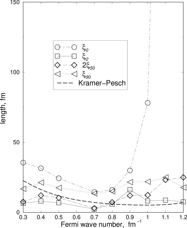
Figure 6: Various length scales for a vortex as a function of the density. The meaning of the different symbols are explained in the text.

Figure 6 shows the relevant lengths for the case of polarized gap. The lengths remain limited ($<15$ fm) for essentially all densities and tend to decrease at higher density. This behavior is different from the BCS coherence length $\xi_{0}$ which scales like $k_{F}/\Delta_{\infty}$. In the realistic case where the pairing strength is fitted to the gap in uniform matter, the coherence length $\xi_{2}$ decreases as a function of $k_{F}$. Thus, the density dependence of the pairing strength $|g|$ is also very important, and the vortex size appears to depend in a quite complex way on both $|g|$ and the Fermi wavenumber. In the figure we also show the analytic estimate of the vortex core size made by Kramer & Pesch (1974) whose value in our units (energies in MeV and lengths in fm) is

$$\xi_{1}={661.3\over k_{F}^{2}|g|}.$$ (48)

Since the pinning force between a nucleus and a vortex behaves like $\sim\Delta^{2}k_{F}/\xi_{2}$, an increase of the pinning force of the order $\sim\xi_{0}/\xi_{2}$ can be expected. In addition we can confirm what we found in Paper I, that since the diameter of the vortex is always smaller than the lattice spacing, the vortex envelops at most one nucleus along a plane perpendicular to its axis.

Another interesting parameter is represented by the coherent flux of neutrons in the presence of a vortex. The flux is given by

$$J({\bf r})={\hbar\over 2mi}{\biggl{(}}\sum_{i}{\biggl{[}}V_{i}({\bf r})\nabla V^{*}_{i}({\bf r})-V^{*}_{i}({\bf r})\nabla V_{i}({\bf r}){\biggr{]}}(1-f(E_{i}))+{\biggl{[}}U_{i}({\bf r})\nabla U^{*}_{i}({\bf r})-U^{*}_{i}({\bf r})\nabla U_{i}({\bf r}){\biggr{]}}(1-f(E_{i})){\biggr{)}}$$ (49)

which in the present case becomes

$$J(\rho)={\hbar\over 2m\rho}{\biggl{[}}\sum_{E_{i}<0}(\mu-1/2)(|u_{i}({\rho})|^{2}-\sum_{E_{i}>0}(\mu+1/2)|v_{i}({\rho})|^{2}{\biggr{]}}.$$ (50)

Figure 7 shows the flux of neutrons with and without a nucleus present in the middle of the cell for the case of $k_{F}=0.4$ fm^-1. The main effect of the nucleus is to decrease the flux. The coherent velocity field can be obtained dividing the flux by the neutron density. In this case the velocity is even more depleted in the centre due to the much higher density in the nuclear region than outside, a situation typical for low values of $k_{F}$.

3.3 Variations in $\Delta$ due to a center of scattering

Pinning or antipinning between a vortex and a nucleus is due to local variations in both the kinetic energy density and the condensation energy. Although pinning will be examined in detail in a next section, it is interesting to study how the pairing gap changes in the cell when a nucleus alone is present. Some curves have already been presented in Figure 1, but here we shall be more systematic discussing of the applications to pinning calculations. The variation of the pairing gap as a function of the distance from the axis of a cylindrical nucleus when the vortex is absent can be seen in Figure 8 for some selected densities. Note that the presence of a mean field decreases the value of the gap. This is mainly due to the increase of the density in the nuclear region, since the pairing force $|g|$ depends on the local density. Note also that the variation of the gap extends beyond the range of the mean field, indicated with a dashed line. This is due in part to the long tail of the density distribution beyond the radius of the potential, an effect due to the presence of scattering states. Secondly, there is a proximity effect between the nuclear region and the free neutron gas due to Andreev scattering (that is, scattering due to spatial variations the pairing potential) of quasi-particles.

3.4 Pinning energy and vortex self-energy

The vortex self-energy or tension $T$, which is the energy carried by the vortex per unit length, is a relevant parameter for vortex-nucleus pinning. Let us consider the behavior of a single vortex line in interaction with the whole lattice. If the energy necessary for the vortex to reach the pinning centers is very high compared to the energy gained by pinning, the vortex responds stiffly to local deformations. The importance of this parameter can be grasped in a limiting case: for $T\rightarrow\infty$ the vortex behaves like a rigid cylinder. For a vortex moving perpendicularly to its axis the total pinning force with the lattice arises from stochastic summation from all the pinning centers and is proportional to the square root of the vortex length (see for example Tinkham (1996) for the case of superconductors). Thus, the pinning force cannot balance the Magnus force, which increases linearly with the vortex length. If this was the case, the pinning mechanism would not be effective for storing the energy released during a glitch (Anderson & Itoh (1975)). For a finite stiffness, the situation is more complicated. Solving the equation of motion for a vortex line passing through many centers of pinning would give the value of the total pinning energy which is able to be stored, but this is a difficult task due to the difficulty in finding the appropriate boundary conditions in the presence of many centers of pinning. It has been argued that although finite, the tension is too large to account for large glitches (Jones (1998)). If, on the other hand, the pinning model is correct, the value of the vortex tension is relevant for the dynamics of unpinning (Link & Epstein (1995)) and for the value of the effective pinning force per unit length.

The vortex tension is the energy difference per unit length between the configuration with and without a vortex, $T=\left[E({\rm vortex})-E({\rm uniform\;matter})\right]/L.$ To calculate the energy of the superfluid in each configuration one can take averages of Eq. (6). The result is

$$E=\int d^{3}r{|\Delta({\bf r})|^{2}\over|g|}+2\sum_{E_{n}<0}E_{n}-2\sum_{E_{n}}E_{n}\int d^{3}r|V_{n}({\bf r})|^{2}.$$ (51)

Table (2) shows the calculated points as a function of the Fermi wave number compared to the classical calculation where the kinetic energy density is integrated from the coherence length $\xi$ up to an upper limit $R_{0}$:

$$T=4.38k_{F}^{3}\ln{\biggl{(}}{R_{0}\over\xi}{\biggr{)}}.$$ (52)

Evidently the presence of bound states does not change the vortex tension radically. Furthermore, constraining the vortex in a small cylinder can overestimate the role of bound states in the calculation of self-energy, because the vortex is macroscopic along the $\rho$ direction. We also expect that uncertainties in the pairing gap or in the cutoff length $R_{0}$ (that should be of the order of the vortex-vortex separation) may be much greater than the discrepancy we find between our microscopic calculations and the estimate (52). We conclude that equation (52) is reliable when applied to vortex calculations in a neutron star. Assuming a vortex-vortex separation of the order $R_{0}\sim 10^{-2}$ cm, this formula implies a tension of the order $T\sim 10^{9}$ erg cm^-1 at $k_{F}=0.8$ fm^-1. At such values a vortex can deform only at length scales of the order of several hundreds of fm, nearly $20$ times larger than the lattice spacing, unless the pinning energy assumes unrealistically large values. How a vortex line with such small deformability can adapt its shape to gain a net pinning energy is still an unsolved problem (Jones (1997)). We show in the following that an answer may be provided by the high value of the elementary pinning force.

To calculate the pinning energy we need to consider four different configurations: a vortex superimposed on a nucleus, an isolated nucleus, an isolated vortex, and finally uniform matter. For each configuration, the energy needs to be calculated with Eq. (51). The pinning energy per unit length can be calculated as

$$E_{p}={\biggl{[}}E({\rm nucleus\;and\;vortex})-E({\rm nucleus})+E({\rm uniform\;matter})-E({\rm vortex}){\biggr{]}}/L.$$ (53)

Table (3) collects some pinning data calculated with Eq. (49) and (51). A negative sign corresponds to a pinning situation in which it is energetically favorable for a vortex to remain attached to a nucleus, while a positive sign indicates an antipinning situation, where vortices are repelled by nuclei. We find an antipinning-pinning transition at $k_{F}=0.30-0.40$ fm^-1. A similar transition was found in a Ginzburg-Landau approach (Epstein & Baym (1988)). The pinning energy reaches values of the order of several MeV per unit length, corresponding to a very high value if compared to previous calculations performed solely on the basis of the condensation energy loss. As is also found in other models where the kinetic energy is accounted for (Epstein & Baym (1988)), part of these large values can be attributed to kinetic energy effects. For such large values of the pinning energy a vortex is likely to deform sensitively in order to be able to catch the pinning centers. In addition, the ions in the lattice will shift to the vortex in response to the high pinning force, a situation referred to as superstrong pinning. Since nuclei in most of the crust are spherical, one might question the applicability of our calculations, where nuclei are considered to be cylindrical. Although the proper use of spherical geometry would, of course, quantitatively change the results, we do not expect dramatic differences.

4 Conclusions

The results presented in this paper could be a step towards an understanding of vortex structure and interaction in neutron star crusts. We have found differences between the predictions of microscopic theory and those of more macroscopic models. In particular, we showed that the BCS coherence length cannot be used as a reliable estimate of the vortex core size, especially not at low and intermediate densities. By solving the self-consistent problem of a vortex in neutron matter, we have shown that the vortex core has a much more complicated structure than that which is usually assumed in simplified treatments of the problem, e.g.: 1) the gap changes from zero at the axis of the core up to an asymptotic value, and 2): there are bound states present.

We found that vortices in neutron star matter follow a behavior similar to that described by Kramer & Pesch (1974) for superconductors, namely, at zero temperature the vortex core size scales as the inverse of the Fermi wave number. In a superconductor in clean limit this effect is associated with a linear increase of the vortex core size with temperature. We have not investigated the temperature dependence of our results, because this is not very relevant in neutron star physics due to the low temperatures compared with the Fermi energy. Unfortunately, experimental data for clean type II superconductors are limited to the quite complex new cuprate systems. Scanning tunnelling microscopy has, however, confirmed the presence of bound states of quasiparticles in the vortex core, in good agreement with the Bogoljubov-de Gennes theory. In view of the small range of the nuclear force and of the simple structure of the Fermi surface, the BdG model could be a very good approximation for neutron star matter.

High pinning energies and small lengths imply a large pinning (or anti-pinning) force. In addition, the small value of the coherence length means that a vortex envelopes no more than one nucleus in a plane perpendicular to the vortex axis. The possibility for a vortex to store pinning energy is largely the result of a competition between the energy gain with pinning and the energy cost to deform. To be able to deform and catch a nucleus along its path, a vortex has to be relatively free to perform local deformations. Assuming that the energy of the vortex is solely due to kinetic effects, the tension turns out to be of the order $T\approx 100k_{F}^{3}$ MeV fm^-1 and is thus very high at densities corresponding to the deep inner crust. For a total pinning energy per nucleus $E_{p}$, a vortex can efficiently catch the pinning sites only if they are at least a distance $\approx a^{2}T/2$ apart. For example, at $k_{F}=1$ fm^-1 a vortex deformation of the order of the lattice spacing can occur every $\sim 8$ or so lattice spacings, while at $k_{F}=0.8$ fm^-1 the pinning efficiency would be much better. Calculations of the geometry of vortex deformation in a one-dimensional crystalline structure have been performed by (Link & Epstein (1995)).

Finally, there are other unsolved problems in neutron star dynamics where a microscopic description of vortex states might prove helpful. The scattering of electrons off neutron vortices results in a coupling between protons and neutrons in the interior of the star. This is a possible coupling mode between the superfluid neutrons and the rest of the star, and depends on the microscopic structure of vortex lines (Sauls (1989)).

The proton vortices in the interior of the star induced by the rotation will probably be similar to the neutron vortices examined in this paper, but additionally they will generate a magnetic field parallel to the rotational axis. How these magnetic vortices interact with the (much more numerous) flux tubes induced by the high magnetic field penetrating into the star is only one of the problems connected to the dynamics of superfluid vortices below the star’s crust. Despite their importance in the evolution of the pulsar’s magnetic field, the properties of proton flux tubes and their possible interaction with neutron vortices in the interior, where neutrons couple in a triplet phase, are not well understood (Ruderman (1997)). A microscopic description of proton flux lines might also be applied to the study uf ultra-high magnetic fields and the evolution of magnetic field in magnetars.

Table 1: Gap at infinity $\Delta_{\infty}$ and the length scales $\xi_{0}$, $\xi_{2}$, $\xi_{90}$ and $2\xi_{50}$ for different values of the Fermi wave number and pairing gaps.

$k_{F}\;({\rm fm}^{-1}$)	$\Delta_{\infty}$	$\xi_{0}$ (fm)	$\xi_{2}$ (fm)	$\xi_{90}$ (fm)	2$\xi_{50}$ (fm)
0.1	0.0049	344.9	6.02	11.11	7.15
0.1	0.011	153.4	6.07	19.89	12.29
0.2	0.02	152.0	9.80	15.61	11.03
0.2	0.04	81.83	12.73	16.56	13.20
0.2	0.183	18.41	5.57	8.04	6.04
0.2	0.291	11.57	5.20	7.13	5.63
0.2	0.744	4.54	4.59	6.18	4.96
0.5	0.226	37.34	5.32	17.71	7.266
0.5	0.778	10.71	2.96	9.13	3.33
0.5	1.73	4.87	2.52	6.75	2.67
0.5	3.42	2.46	2.09	3.24	3.02
0.8	0.205	65.8	6.05	24.60	17.48
0.8	1.72	7.84	2.21	9.21	2.65
0.8	3.8	3.55	1.67	5.02	1.87

Table 2: Vortex self-energy $T$ (in MeV fm^-1) at different Fermi wave numbers calculated from the program and the value $T_{f}$ calculated from the analytical formula, where the coherence length $\xi_{2}$ has been used for the lower length $b$. The radius $R$ of the cylinder is reported.

$k_{F}\;({\rm fm}^{-1}$)	$T$ (MeV fm -1)	$T_{f}$ (MeV fm-1)	$\xi_{0}$ (fm)
0.4	1.08	0.64	80
0.5	1.03	1.344	80
0.7	1.67	5.30	80
0.85	3.06	7.401	60

Table 3: The pinning energy per unit length $E_{p}$ (in MeV fm^-1) at different Fermi wave numbers calculated for a potential well with the following parameters: radius $R_{N}=5$ fm, depth $W=-30$ MeV and diffusivity $a=0.6$ fm. The radius $R$ of the cylinder is $80$ fm.

$k_{F}\;({\rm fm}^{-1}$)	$E_{p}$ (MeV fm-1)
0.15	0.68
0.20	0.201
0.30	-0.091
0.5	-0.77
0.7	-2.34
0.85	-16.47
1.00	-4.09

Figure 1: Pairing potential $\Delta(\rho)$ as a function of the distance $\rho$ from the symmetry axis of the vortex with a pairing force independent of the density and fixed to return the desired value of the gap at infinity.

Figure 2: The eigenvalues of the BdG equations for a vortex in neutron matter for the case $k_{F}=0.8$ and a pairing gap at infinity $\Delta_{\infty}$=2.9 MeV. The positive and negative quasiparticle states in the continuum are separated by a gap equal to $2\Delta_{\infty}$. The bound states are visible as the branch between the continuum states. Only one single value of $k_{z}=0$ has been included in the calculation.

Figure 3: Distribution of energy eigenvalues as a function of angular momentum, now also with different values for $k_{z}$. $\Delta_{\infty}=0.5$ MeV and $k_{F}=0.22$.

Figure 4: Pairing potential $\Delta(\rho)$ as a function of $\rho$ for three different situations. The density of uniform matter is in all three cases given by $k_{F}=0.8\;{\rm fm}^{-1}$.

Figure 5: Density distribution $n(\rho)$ as a function of $\rho$ for three different situations. The density of uniform matter is in all cases given by $k_{F}=0.8\;{\rm fm}^{-1}$.

Figure 7: The coherent velocity field for a vortex with and without a center of scattering.

Figure 8: Pairing potential at various densities for the case of a nucleus immersed in a homogeneous (vortex-free) neutron superfluid.