Turbulent Dynamos and Magnetic Helicity

Abstract

It is shown that the turbulent dynamo $\alpha$-effect converts magnetic helicity from the turbulent field to the mean field when the turbulence is electromagnetic while the magnetic helicity of the mean-field is transported across space when the turbulence is electrostatic or due to the electron diamagnetic effect. In all cases, however, the dynamo effect strictly conserves the total helicity except for resistive effects and a small battery effect. Implications for astrophysical situations, especially for the solar dynamo, are discussed.

Magnetic fields are observed to exist not only in the planets and the stars [1] but essentially everywhere in the universe, such as the interstellar medium in galaxies and even in clusters of galaxies [2]. The origin of these cosmical magnetic fields has been explained mainly by dynamo theory [3], which is one of the most active research areas across multiple subdisciplines of physics. In particular, generation of an electromotive force (EMF) along a mean field by turbulence, or the well-known $\alpha$ effect [4], is an essential process in amplifying large-scale magnetic fields [5]. Experimentally, the $\alpha$ effect has been observed in toroidal laboratory plasmas [6].

Recently, there has been growing awareness that a topological constraint on the observed magnetic field, the conservation of magnetic helicity, may play an important role in solar flare evolution [7]. This follows the success of Taylor in explaining the observed magnetic structures in laboratory plasmas by conjecturing the same constraint during relaxation [8]. Magnetic helicity, a measure of the “knottedness”and the “twistedness” of magnetic fields [9, 10], is closely related to the dynamo effect. Indeed, the $\alpha$ effect drives parallel current which twists up the field lines, thus increasing magnetic helicity on large scales. As a matter of fact, almost all the observed large scale cosmical poloidal (or meridional) magnetic fields, either in their dipolar or quadrupolar forms, have linkage with strong toroidal (or azimuthal) fields, leading to finite magnetic helicity.

One simple yet important question arises: how exactly is magnetic helicity affected by the dynamo process? Can magnetic helicity of the large-scale field be created by the dynamo process or merely be transported across space? Motivated by Taylor’s conjecture, early studies [11] showed that the $\alpha$ effect only transports helicity of the large-scale field across space without affecting the total helicity, as supported by laboratory measurements[12]. However, a contradicting conclusion was drawn in a recent study [13], which showed that the $\alpha$ effect locally converts helicity from the turbulent field to the mean field, as supported by statistical and numerical studies on inverse helicity cascading to large scales [14, 15]. Answers to the questions raised by this contradiction are in demand since they would reveal the nature of the dynamo effects and clarify the effectiveness or limitations of the magnetic helicity concept in determining the evolution of solar and laboratory plasmas in which the the dynamo plays a role.

In this Letter, it is shown that both conclusions, i.e. creation or transport of the large-scale magnetic helicity by the $\alpha$ effect, are valid depending on the nature of the turbulence which drives the dynamo effect. When the turbulence is electromagnetic, the $\alpha$ effect converts helicity from the turbulent, small-scale field to the mean, large-scale field. On the other hand, when the turbulence is electrostatic or due to the electron diamagnetic effect, the $\alpha$ effect transports the mean-field helicity across space without dissipation. In all cases, however, the $\alpha$ effect strictly conserves the total helicity except for resistive effects and a small battery effect. Implications for astrophysical situations, especially for the solar dynamo, are discussed.

In order to include other possible dynamo effects in a plasma, we revisit the mean-field electrodynamics [5] using the generalized Ohm’s law (ignoring the electron inertial term) [16]

$${\mathchoice{{\hbox{\boldmath$\displaystyle E$}}}{{\hbox{\boldmath$\textstyle E$}}}{{\hbox{\boldmath$\scriptstyle E$}}}{{\hbox{\boldmath$\scriptscriptstyle E$}}}}+{\mathchoice{{\hbox{\boldmath$\displaystyle v$}}}{{\hbox{\boldmath$\textstyle v$}}}{{\hbox{\boldmath$\scriptstyle v$}}}{{\hbox{\boldmath$\scriptscriptstyle v$}}}}\times{\mathchoice{{\hbox{\boldmath$\displaystyle B$}}}{{\hbox{\boldmath$\textstyle B$}}}{{\hbox{\boldmath$\scriptstyle B$}}}{{\hbox{\boldmath$\scriptscriptstyle B$}}}}-{\mathchoice{{\hbox{\boldmath$\displaystyle j$}}}{{\hbox{\boldmath$\textstyle j$}}}{{\hbox{\boldmath$\scriptstyle j$}}}{{\hbox{\boldmath$\scriptscriptstyle j$}}}}\times{\mathchoice{{\hbox{\boldmath$\displaystyle B$}}}{{\hbox{\boldmath$\textstyle B$}}}{{\hbox{\boldmath$\scriptstyle B$}}}{{\hbox{\boldmath$\scriptscriptstyle B$}}}}/en+\mbox{\boldmath$\nabla$}P_{e}/en=\eta{\mathchoice{{\hbox{\boldmath$\displaystyle j$}}}{{\hbox{\boldmath$\textstyle j$}}}{{\hbox{\boldmath$\scriptstyle j$}}}{{\hbox{\boldmath$\scriptscriptstyle j$}}}},$$ (1)

where $n$ is the electron density and $P_{e}$ the electron pressure. Every quantity $x$ is divided into a mean part $\overline{x}\equiv\langle x\rangle$, averaged over ensembles or space, and a turbulent part $\widetilde{x}$: $x=\overline{x}+\widetilde{x}$. Then the mean and turbulent versions of the Ohm’s law become

$$\overline{\mathchoice{{\hbox{\boldmath$\displaystyle E$}}}{{\hbox{\boldmath$\textstyle E$}}}{{\hbox{\boldmath$\scriptstyle E$}}}{{\hbox{\boldmath$\scriptscriptstyle E$}}}}+\overline{\mathchoice{{\hbox{\boldmath$\displaystyle v$}}}{{\hbox{\boldmath$\textstyle v$}}}{{\hbox{\boldmath$\scriptstyle v$}}}{{\hbox{\boldmath$\scriptscriptstyle v$}}}}_{e}\times\overline{\mathchoice{{\hbox{\boldmath$\displaystyle B$}}}{{\hbox{\boldmath$\textstyle B$}}}{{\hbox{\boldmath$\scriptstyle B$}}}{{\hbox{\boldmath$\scriptscriptstyle B$}}}}+{\mbox{\boldmath$\nabla$}\overline{P}_{e}/en}+\mbox{\boldmath$\mathcal{E}$} = \eta\overline{\mathchoice{{\hbox{\boldmath$\displaystyle j$}}}{{\hbox{\boldmath$\textstyle j$}}}{{\hbox{\boldmath$\scriptstyle j$}}}{{\hbox{\boldmath$\scriptscriptstyle j$}}}}$$ (2)

$$\widetilde{\mathchoice{{\hbox{\boldmath$\displaystyle E$}}}{{\hbox{\boldmath$\textstyle E$}}}{{\hbox{\boldmath$\scriptstyle E$}}}{{\hbox{\boldmath$\scriptscriptstyle E$}}}}+\widetilde{\mathchoice{{\hbox{\boldmath$\displaystyle v$}}}{{\hbox{\boldmath$\textstyle v$}}}{{\hbox{\boldmath$\scriptstyle v$}}}{{\hbox{\boldmath$\scriptscriptstyle v$}}}}_{e}\times\overline{\mathchoice{{\hbox{\boldmath$\displaystyle B$}}}{{\hbox{\boldmath$\textstyle B$}}}{{\hbox{\boldmath$\scriptstyle B$}}}{{\hbox{\boldmath$\scriptscriptstyle B$}}}}+(\overline{\mathchoice{{\hbox{\boldmath$\displaystyle v$}}}{{\hbox{\boldmath$\textstyle v$}}}{{\hbox{\boldmath$\scriptstyle v$}}}{{\hbox{\boldmath$\scriptscriptstyle v$}}}}_{e}+\widetilde{\mathchoice{{\hbox{\boldmath$\displaystyle v$}}}{{\hbox{\boldmath$\textstyle v$}}}{{\hbox{\boldmath$\scriptstyle v$}}}{{\hbox{\boldmath$\scriptscriptstyle v$}}}}_{e})\times\widetilde{\mathchoice{{\hbox{\boldmath$\displaystyle B$}}}{{\hbox{\boldmath$\textstyle B$}}}{{\hbox{\boldmath$\scriptstyle B$}}}{{\hbox{\boldmath$\scriptscriptstyle B$}}}}-\mbox{\boldmath$\mathcal{E}$}+{\mbox{\boldmath$\nabla$}\widetilde{P}_{e}/en} = \eta\widetilde{\mathchoice{{\hbox{\boldmath$\displaystyle j$}}}{{\hbox{\boldmath$\textstyle j$}}}{{\hbox{\boldmath$\scriptstyle j$}}}{{\hbox{\boldmath$\scriptscriptstyle j$}}}},$$ (3)

where ${\mathchoice{{\hbox{\boldmath$\displaystyle v$}}}{{\hbox{\boldmath$\textstyle v$}}}{{\hbox{\boldmath$\scriptstyle v$}}}{{\hbox{\boldmath$\scriptscriptstyle v$}}}}_{i}$ (${\mathchoice{{\hbox{\boldmath$\displaystyle v$}}}{{\hbox{\boldmath$\textstyle v$}}}{{\hbox{\boldmath$\scriptstyle v$}}}{{\hbox{\boldmath$\scriptscriptstyle v$}}}}_{e}$) is the ion (electron) flow velocity and the relations ${\mathchoice{{\hbox{\boldmath$\displaystyle v$}}}{{\hbox{\boldmath$\textstyle v$}}}{{\hbox{\boldmath$\scriptstyle v$}}}{{\hbox{\boldmath$\scriptscriptstyle v$}}}}\approx{\mathchoice{{\hbox{\boldmath$\displaystyle v$}}}{{\hbox{\boldmath$\textstyle v$}}}{{\hbox{\boldmath$\scriptstyle v$}}}{{\hbox{\boldmath$\scriptscriptstyle v$}}}}_{i}$ and ${\mathchoice{{\hbox{\boldmath$\displaystyle j$}}}{{\hbox{\boldmath$\textstyle j$}}}{{\hbox{\boldmath$\scriptstyle j$}}}{{\hbox{\boldmath$\scriptscriptstyle j$}}}}=en({\mathchoice{{\hbox{\boldmath$\displaystyle v$}}}{{\hbox{\boldmath$\textstyle v$}}}{{\hbox{\boldmath$\scriptstyle v$}}}{{\hbox{\boldmath$\scriptscriptstyle v$}}}}_{i}-{\mathchoice{{\hbox{\boldmath$\displaystyle v$}}}{{\hbox{\boldmath$\textstyle v$}}}{{\hbox{\boldmath$\scriptstyle v$}}}{{\hbox{\boldmath$\scriptscriptstyle v$}}}}_{e})$ have been used. The mean EMF $\mathcal{E}$ is given by

$$\mbox{\boldmath$\mathcal{E}$}=\langle\widetilde{\mathchoice{{\hbox{\boldmath$\displaystyle v$}}}{{\hbox{\boldmath$\textstyle v$}}}{{\hbox{\boldmath$\scriptstyle v$}}}{{\hbox{\boldmath$\scriptscriptstyle v$}}}}\times\widetilde{\mathchoice{{\hbox{\boldmath$\displaystyle B$}}}{{\hbox{\boldmath$\textstyle B$}}}{{\hbox{\boldmath$\scriptstyle B$}}}{{\hbox{\boldmath$\scriptscriptstyle B$}}}}\rangle-\langle\widetilde{\mathchoice{{\hbox{\boldmath$\displaystyle j$}}}{{\hbox{\boldmath$\textstyle j$}}}{{\hbox{\boldmath$\scriptstyle j$}}}{{\hbox{\boldmath$\scriptscriptstyle j$}}}}\times\widetilde{\mathchoice{{\hbox{\boldmath$\displaystyle B$}}}{{\hbox{\boldmath$\textstyle B$}}}{{\hbox{\boldmath$\scriptstyle B$}}}{{\hbox{\boldmath$\scriptscriptstyle B$}}}}\rangle/en\approx\langle\widetilde{\mathchoice{{\hbox{\boldmath$\displaystyle v$}}}{{\hbox{\boldmath$\textstyle v$}}}{{\hbox{\boldmath$\scriptstyle v$}}}{{\hbox{\boldmath$\scriptscriptstyle v$}}}}_{e}\times\widetilde{\mathchoice{{\hbox{\boldmath$\displaystyle B$}}}{{\hbox{\boldmath$\textstyle B$}}}{{\hbox{\boldmath$\scriptstyle B$}}}{{\hbox{\boldmath$\scriptscriptstyle B$}}}}\rangle.$$ (4)

(Small battery-like effects such as $\langle\widetilde{n}\mbox{\boldmath$\nabla$}\widetilde{P}_{e}\rangle/e\overline{n}^{2}$ are neglected; see discussions later.) The appearance of ${\mathchoice{{\hbox{\boldmath$\displaystyle v$}}}{{\hbox{\boldmath$\textstyle v$}}}{{\hbox{\boldmath$\scriptstyle v$}}}{{\hbox{\boldmath$\scriptscriptstyle v$}}}}_{e}$ only on the RHS of Eq.(4) is consistent with Ohm’s law being a force balance on electrons.

The parallel component of $\mathcal{E}$, or the $\alpha$-effect [4], along the mean field is of interest via Eq.(3):

$$\mbox{\boldmath$\mathcal{E}$}\cdot\overline{\mathchoice{{\hbox{\boldmath$\displaystyle B$}}}{{\hbox{\boldmath$\textstyle B$}}}{{\hbox{\boldmath$\scriptstyle B$}}}{{\hbox{\boldmath$\scriptscriptstyle B$}}}} = \langle\widetilde{\mathchoice{{\hbox{\boldmath$\displaystyle v$}}}{{\hbox{\boldmath$\textstyle v$}}}{{\hbox{\boldmath$\scriptstyle v$}}}{{\hbox{\boldmath$\scriptscriptstyle v$}}}}_{e}\times\widetilde{\mathchoice{{\hbox{\boldmath$\displaystyle B$}}}{{\hbox{\boldmath$\textstyle B$}}}{{\hbox{\boldmath$\scriptstyle B$}}}{{\hbox{\boldmath$\scriptscriptstyle B$}}}}\rangle\cdot\overline{\mathchoice{{\hbox{\boldmath$\displaystyle B$}}}{{\hbox{\boldmath$\textstyle B$}}}{{\hbox{\boldmath$\scriptstyle B$}}}{{\hbox{\boldmath$\scriptscriptstyle B$}}}}=-\langle(\widetilde{\mathchoice{{\hbox{\boldmath$\displaystyle v$}}}{{\hbox{\boldmath$\textstyle v$}}}{{\hbox{\boldmath$\scriptstyle v$}}}{{\hbox{\boldmath$\scriptscriptstyle v$}}}}_{e}\times\overline{\mathchoice{{\hbox{\boldmath$\displaystyle B$}}}{{\hbox{\boldmath$\textstyle B$}}}{{\hbox{\boldmath$\scriptstyle B$}}}{{\hbox{\boldmath$\scriptscriptstyle B$}}}})\cdot\widetilde{\mathchoice{{\hbox{\boldmath$\displaystyle B$}}}{{\hbox{\boldmath$\textstyle B$}}}{{\hbox{\boldmath$\scriptstyle B$}}}{{\hbox{\boldmath$\scriptscriptstyle B$}}}}\rangle$$ (5)

$$= \langle\widetilde{\mathchoice{{\hbox{\boldmath$\displaystyle E$}}}{{\hbox{\boldmath$\textstyle E$}}}{{\hbox{\boldmath$\scriptstyle E$}}}{{\hbox{\boldmath$\scriptscriptstyle E$}}}}\cdot\widetilde{\mathchoice{{\hbox{\boldmath$\displaystyle B$}}}{{\hbox{\boldmath$\textstyle B$}}}{{\hbox{\boldmath$\scriptstyle B$}}}{{\hbox{\boldmath$\scriptscriptstyle B$}}}}\rangle+\langle\mbox{\boldmath$\nabla$}\widetilde{P}_{e}\cdot\widetilde{\mathchoice{{\hbox{\boldmath$\displaystyle B$}}}{{\hbox{\boldmath$\textstyle B$}}}{{\hbox{\boldmath$\scriptstyle B$}}}{{\hbox{\boldmath$\scriptscriptstyle B$}}}}\rangle/e\overline{n}-\eta\langle\widetilde{\mathchoice{{\hbox{\boldmath$\displaystyle j$}}}{{\hbox{\boldmath$\textstyle j$}}}{{\hbox{\boldmath$\scriptstyle j$}}}{{\hbox{\boldmath$\scriptscriptstyle j$}}}}\cdot\widetilde{\mathchoice{{\hbox{\boldmath$\displaystyle B$}}}{{\hbox{\boldmath$\textstyle B$}}}{{\hbox{\boldmath$\scriptstyle B$}}}{{\hbox{\boldmath$\scriptscriptstyle B$}}}}\rangle,$$ (6)

where the last term diminishes in the limit of small resistivity [14, 17] and shall be discussed later. The first term $\langle\widetilde{\mathchoice{{\hbox{\boldmath$\displaystyle E$}}}{{\hbox{\boldmath$\textstyle E$}}}{{\hbox{\boldmath$\scriptstyle E$}}}{{\hbox{\boldmath$\scriptscriptstyle E$}}}}\cdot\widetilde{\mathchoice{{\hbox{\boldmath$\displaystyle B$}}}{{\hbox{\boldmath$\textstyle B$}}}{{\hbox{\boldmath$\scriptstyle B$}}}{{\hbox{\boldmath$\scriptscriptstyle B$}}}}\rangle$ represents the contribution to $\widetilde{\mathchoice{{\hbox{\boldmath$\displaystyle v$}}}{{\hbox{\boldmath$\textstyle v$}}}{{\hbox{\boldmath$\scriptstyle v$}}}{{\hbox{\boldmath$\scriptscriptstyle v$}}}}_{e}$ from the turbulent $\widetilde{\mathchoice{{\hbox{\boldmath$\displaystyle E$}}}{{\hbox{\boldmath$\textstyle E$}}}{{\hbox{\boldmath$\scriptstyle E$}}}{{\hbox{\boldmath$\scriptscriptstyle E$}}}}\times\overline{\mathchoice{{\hbox{\boldmath$\displaystyle B$}}}{{\hbox{\boldmath$\textstyle B$}}}{{\hbox{\boldmath$\scriptstyle B$}}}{{\hbox{\boldmath$\scriptscriptstyle B$}}}}$ drift which is a single fluid (MHD) effect [18], while the second term, $\langle\mbox{\boldmath$\nabla$}\widetilde{P}_{e}\cdot\widetilde{\mathchoice{{\hbox{\boldmath$\displaystyle B$}}}{{\hbox{\boldmath$\textstyle B$}}}{{\hbox{\boldmath$\scriptstyle B$}}}{{\hbox{\boldmath$\scriptscriptstyle B$}}}}\rangle/en$, is the contribution from the turbulent electron diamagnetic drift $\mbox{\boldmath$\nabla$}\widetilde{P}_{e}\times\overline{\mathchoice{{\hbox{\boldmath$\displaystyle B$}}}{{\hbox{\boldmath$\textstyle B$}}}{{\hbox{\boldmath$\scriptstyle B$}}}{{\hbox{\boldmath$\scriptscriptstyle B$}}}}$ which is an electron fluid effect [19].

In general, the electric field can be split further into a curl-free part and a divergence-free part, often called “electrostatic”and “electromagnetic”, respectively: ${\mathchoice{{\hbox{\boldmath$\displaystyle E$}}}{{\hbox{\boldmath$\textstyle E$}}}{{\hbox{\boldmath$\scriptstyle E$}}}{{\hbox{\boldmath$\scriptscriptstyle E$}}}}=-\mbox{\boldmath$\nabla$}\phi-\partial{\mathchoice{{\hbox{\boldmath$\displaystyle A$}}}{{\hbox{\boldmath$\textstyle A$}}}{{\hbox{\boldmath$\scriptstyle A$}}}{{\hbox{\boldmath$\scriptscriptstyle A$}}}}/\partial t$ where $\textstyle A$ is the vector potential and $\phi$ is the electrostatic potential. Then Eq.(6) becomes

$$\mbox{\boldmath$\mathcal{E}$}\cdot\overline{\mathchoice{{\hbox{\boldmath$\displaystyle B$}}}{{\hbox{\boldmath$\textstyle B$}}}{{\hbox{\boldmath$\scriptstyle B$}}}{{\hbox{\boldmath$\scriptscriptstyle B$}}}}= - \langle\mbox{\boldmath$\nabla$}\widetilde{\phi}\cdot\widetilde{\mathchoice{{\hbox{\boldmath$\displaystyle B$}}}{{\hbox{\boldmath$\textstyle B$}}}{{\hbox{\boldmath$\scriptstyle B$}}}{{\hbox{\boldmath$\scriptscriptstyle B$}}}}\rangle-\langle(\partial\widetilde{\mathchoice{{\hbox{\boldmath$\displaystyle A$}}}{{\hbox{\boldmath$\textstyle A$}}}{{\hbox{\boldmath$\scriptstyle A$}}}{{\hbox{\boldmath$\scriptscriptstyle A$}}}}/\partial t)\cdot\widetilde{\mathchoice{{\hbox{\boldmath$\displaystyle B$}}}{{\hbox{\boldmath$\textstyle B$}}}{{\hbox{\boldmath$\scriptstyle B$}}}{{\hbox{\boldmath$\scriptscriptstyle B$}}}}\rangle$$ (7)

$$+ \langle\mbox{\boldmath$\nabla$}\widetilde{P}_{e}\cdot\widetilde{\mathchoice{{\hbox{\boldmath$\displaystyle B$}}}{{\hbox{\boldmath$\textstyle B$}}}{{\hbox{\boldmath$\scriptstyle B$}}}{{\hbox{\boldmath$\scriptscriptstyle B$}}}}\rangle/en-\eta\langle\widetilde{\mathchoice{{\hbox{\boldmath$\displaystyle j$}}}{{\hbox{\boldmath$\textstyle j$}}}{{\hbox{\boldmath$\scriptstyle j$}}}{{\hbox{\boldmath$\scriptscriptstyle j$}}}}\cdot\widetilde{\mathchoice{{\hbox{\boldmath$\displaystyle B$}}}{{\hbox{\boldmath$\textstyle B$}}}{{\hbox{\boldmath$\scriptstyle B$}}}{{\hbox{\boldmath$\scriptscriptstyle B$}}}}\rangle,$$ (8)

where the first three terms correspond to effects due to electrostatic, electromagnetic, and electron diamagnetic turbulence, respectively [20]. We shall see below that the type of turbulence is crucial in assessing effects of dynamo action on the magnetic helicity.

Magnetic helicity [9] in a volume $V$ is defined [21] by $K=\int{\mathchoice{{\hbox{\boldmath$\displaystyle A$}}}{{\hbox{\boldmath$\textstyle A$}}}{{\hbox{\boldmath$\scriptstyle A$}}}{{\hbox{\boldmath$\scriptscriptstyle A$}}}}\cdot{\mathchoice{{\hbox{\boldmath$\displaystyle B$}}}{{\hbox{\boldmath$\textstyle B$}}}{{\hbox{\boldmath$\scriptstyle B$}}}{{\hbox{\boldmath$\scriptscriptstyle B$}}}}dV$ and its rate of change is given by

$${dK\over dt}=-2\int{\mathchoice{{\hbox{\boldmath$\displaystyle E$}}}{{\hbox{\boldmath$\textstyle E$}}}{{\hbox{\boldmath$\scriptstyle E$}}}{{\hbox{\boldmath$\scriptscriptstyle E$}}}}\cdot{\mathchoice{{\hbox{\boldmath$\displaystyle B$}}}{{\hbox{\boldmath$\textstyle B$}}}{{\hbox{\boldmath$\scriptstyle B$}}}{{\hbox{\boldmath$\scriptscriptstyle B$}}}}dV-\int(2\phi{\mathchoice{{\hbox{\boldmath$\displaystyle B$}}}{{\hbox{\boldmath$\textstyle B$}}}{{\hbox{\boldmath$\scriptstyle B$}}}{{\hbox{\boldmath$\scriptscriptstyle B$}}}}+{\mathchoice{{\hbox{\boldmath$\displaystyle A$}}}{{\hbox{\boldmath$\textstyle A$}}}{{\hbox{\boldmath$\scriptstyle A$}}}{{\hbox{\boldmath$\scriptscriptstyle A$}}}}\times{\partial{\mathchoice{{\hbox{\boldmath$\displaystyle A$}}}{{\hbox{\boldmath$\textstyle A$}}}{{\hbox{\boldmath$\scriptstyle A$}}}{{\hbox{\boldmath$\scriptscriptstyle A$}}}}\over\partial t})\cdot d{\mathchoice{{\hbox{\boldmath$\displaystyle S$}}}{{\hbox{\boldmath$\textstyle S$}}}{{\hbox{\boldmath$\scriptstyle S$}}}{{\hbox{\boldmath$\scriptscriptstyle S$}}}},$$ (9)

where $V$ is enclosed by the surface $\textstyle S$. The integral under the volume integration represents the volume rate of change of helicity, while the integral under the surface integration represents flux of helicity. We note that only the volume term can possibly create or destroy helicity, and the surface terms merely transport helicity across space without affecting the total helicity. The mean helicity $\langle K\rangle$ is the sum of the helicity in the mean field, $K_{\rm m}=\int\overline{\mathchoice{{\hbox{\boldmath$\displaystyle A$}}}{{\hbox{\boldmath$\textstyle A$}}}{{\hbox{\boldmath$\scriptstyle A$}}}{{\hbox{\boldmath$\scriptscriptstyle A$}}}}\cdot\overline{\mathchoice{{\hbox{\boldmath$\displaystyle B$}}}{{\hbox{\boldmath$\textstyle B$}}}{{\hbox{\boldmath$\scriptstyle B$}}}{{\hbox{\boldmath$\scriptscriptstyle B$}}}}dV$, and the helicity in the turbulent field, $K_{\rm t}=\int\langle\widetilde{\mathchoice{{\hbox{\boldmath$\displaystyle A$}}}{{\hbox{\boldmath$\textstyle A$}}}{{\hbox{\boldmath$\scriptstyle A$}}}{{\hbox{\boldmath$\scriptscriptstyle A$}}}}\cdot\widetilde{\mathchoice{{\hbox{\boldmath$\displaystyle B$}}}{{\hbox{\boldmath$\textstyle B$}}}{{\hbox{\boldmath$\scriptstyle B$}}}{{\hbox{\boldmath$\scriptscriptstyle B$}}}}\rangle dV$. From Eq.(9), we have

$${dK_{\rm m}\over dt}= - 2\int\overline{\mathchoice{{\hbox{\boldmath$\displaystyle E$}}}{{\hbox{\boldmath$\textstyle E$}}}{{\hbox{\boldmath$\scriptstyle E$}}}{{\hbox{\boldmath$\scriptscriptstyle E$}}}}\cdot\overline{\mathchoice{{\hbox{\boldmath$\displaystyle B$}}}{{\hbox{\boldmath$\textstyle B$}}}{{\hbox{\boldmath$\scriptstyle B$}}}{{\hbox{\boldmath$\scriptscriptstyle B$}}}}dV-\int(2\bar{\phi}\overline{\mathchoice{{\hbox{\boldmath$\displaystyle B$}}}{{\hbox{\boldmath$\textstyle B$}}}{{\hbox{\boldmath$\scriptstyle B$}}}{{\hbox{\boldmath$\scriptscriptstyle B$}}}}+\overline{\mathchoice{{\hbox{\boldmath$\displaystyle A$}}}{{\hbox{\boldmath$\textstyle A$}}}{{\hbox{\boldmath$\scriptstyle A$}}}{{\hbox{\boldmath$\scriptscriptstyle A$}}}}\times{\partial\overline{\mathchoice{{\hbox{\boldmath$\displaystyle A$}}}{{\hbox{\boldmath$\textstyle A$}}}{{\hbox{\boldmath$\scriptstyle A$}}}{{\hbox{\boldmath$\scriptscriptstyle A$}}}}\over\partial t})\cdot d{\mathchoice{{\hbox{\boldmath$\displaystyle S$}}}{{\hbox{\boldmath$\textstyle S$}}}{{\hbox{\boldmath$\scriptstyle S$}}}{{\hbox{\boldmath$\scriptscriptstyle S$}}}}$$ (10)

$${dK_{\rm t}\over dt}= - 2\int\langle\widetilde{\mathchoice{{\hbox{\boldmath$\displaystyle E$}}}{{\hbox{\boldmath$\textstyle E$}}}{{\hbox{\boldmath$\scriptstyle E$}}}{{\hbox{\boldmath$\scriptscriptstyle E$}}}}\cdot\widetilde{\mathchoice{{\hbox{\boldmath$\displaystyle B$}}}{{\hbox{\boldmath$\textstyle B$}}}{{\hbox{\boldmath$\scriptstyle B$}}}{{\hbox{\boldmath$\scriptscriptstyle B$}}}}\rangle dV-\int\langle 2\widetilde{\phi}\widetilde{\mathchoice{{\hbox{\boldmath$\displaystyle B$}}}{{\hbox{\boldmath$\textstyle B$}}}{{\hbox{\boldmath$\scriptstyle B$}}}{{\hbox{\boldmath$\scriptscriptstyle B$}}}}+\widetilde{\mathchoice{{\hbox{\boldmath$\displaystyle A$}}}{{\hbox{\boldmath$\textstyle A$}}}{{\hbox{\boldmath$\scriptstyle A$}}}{{\hbox{\boldmath$\scriptscriptstyle A$}}}}\times{\partial\widetilde{\mathchoice{{\hbox{\boldmath$\displaystyle A$}}}{{\hbox{\boldmath$\textstyle A$}}}{{\hbox{\boldmath$\scriptstyle A$}}}{{\hbox{\boldmath$\scriptscriptstyle A$}}}}\over\partial t}\rangle\cdot d{\mathchoice{{\hbox{\boldmath$\displaystyle S$}}}{{\hbox{\boldmath$\textstyle S$}}}{{\hbox{\boldmath$\scriptstyle S$}}}{{\hbox{\boldmath$\scriptscriptstyle S$}}}},$$ (11)

where substitution of $\overline{\mathchoice{{\hbox{\boldmath$\displaystyle E$}}}{{\hbox{\boldmath$\textstyle E$}}}{{\hbox{\boldmath$\scriptstyle E$}}}{{\hbox{\boldmath$\scriptscriptstyle E$}}}}$ and $\widetilde{\mathchoice{{\hbox{\boldmath$\displaystyle E$}}}{{\hbox{\boldmath$\textstyle E$}}}{{\hbox{\boldmath$\scriptstyle E$}}}{{\hbox{\boldmath$\scriptscriptstyle E$}}}}$ by Eqs.(2) and (3) yields

$$\overline{\mathchoice{{\hbox{\boldmath$\displaystyle E$}}}{{\hbox{\boldmath$\textstyle E$}}}{{\hbox{\boldmath$\scriptstyle E$}}}{{\hbox{\boldmath$\scriptscriptstyle E$}}}}\cdot\overline{\mathchoice{{\hbox{\boldmath$\displaystyle B$}}}{{\hbox{\boldmath$\textstyle B$}}}{{\hbox{\boldmath$\scriptstyle B$}}}{{\hbox{\boldmath$\scriptscriptstyle B$}}}} = \eta\overline{\mathchoice{{\hbox{\boldmath$\displaystyle j$}}}{{\hbox{\boldmath$\textstyle j$}}}{{\hbox{\boldmath$\scriptstyle j$}}}{{\hbox{\boldmath$\scriptscriptstyle j$}}}}\cdot\overline{\mathchoice{{\hbox{\boldmath$\displaystyle B$}}}{{\hbox{\boldmath$\textstyle B$}}}{{\hbox{\boldmath$\scriptstyle B$}}}{{\hbox{\boldmath$\scriptscriptstyle B$}}}}-\mbox{\boldmath$\mathcal{E}$}\cdot\overline{\mathchoice{{\hbox{\boldmath$\displaystyle B$}}}{{\hbox{\boldmath$\textstyle B$}}}{{\hbox{\boldmath$\scriptstyle B$}}}{{\hbox{\boldmath$\scriptscriptstyle B$}}}}-\mbox{\boldmath$\nabla$}\cdot\left(\overline{P}_{e}\overline{\mathchoice{{\hbox{\boldmath$\displaystyle B$}}}{{\hbox{\boldmath$\textstyle B$}}}{{\hbox{\boldmath$\scriptstyle B$}}}{{\hbox{\boldmath$\scriptscriptstyle B$}}}}/en\right)$$ (12)

$$\langle\widetilde{\mathchoice{{\hbox{\boldmath$\displaystyle E$}}}{{\hbox{\boldmath$\textstyle E$}}}{{\hbox{\boldmath$\scriptstyle E$}}}{{\hbox{\boldmath$\scriptscriptstyle E$}}}}\cdot\widetilde{\mathchoice{{\hbox{\boldmath$\displaystyle B$}}}{{\hbox{\boldmath$\textstyle B$}}}{{\hbox{\boldmath$\scriptstyle B$}}}{{\hbox{\boldmath$\scriptscriptstyle B$}}}}\rangle = \eta\langle\widetilde{\mathchoice{{\hbox{\boldmath$\displaystyle j$}}}{{\hbox{\boldmath$\textstyle j$}}}{{\hbox{\boldmath$\scriptstyle j$}}}{{\hbox{\boldmath$\scriptscriptstyle j$}}}}\cdot\widetilde{\mathchoice{{\hbox{\boldmath$\displaystyle B$}}}{{\hbox{\boldmath$\textstyle B$}}}{{\hbox{\boldmath$\scriptstyle B$}}}{{\hbox{\boldmath$\scriptscriptstyle B$}}}}\rangle+\mbox{\boldmath$\mathcal{E}$}\cdot\overline{\mathchoice{{\hbox{\boldmath$\displaystyle B$}}}{{\hbox{\boldmath$\textstyle B$}}}{{\hbox{\boldmath$\scriptstyle B$}}}{{\hbox{\boldmath$\scriptscriptstyle B$}}}}-\mbox{\boldmath$\nabla$}\cdot\left(\langle\widetilde{P}_{e}\widetilde{\mathchoice{{\hbox{\boldmath$\displaystyle B$}}}{{\hbox{\boldmath$\textstyle B$}}}{{\hbox{\boldmath$\scriptstyle B$}}}{{\hbox{\boldmath$\scriptscriptstyle B$}}}}\rangle/en\right).$$ (13)

It might be concluded that the dynamo effects convert helicity from the turbulent field to the mean field since $\mbox{\boldmath$\mathcal{E}$}\cdot\overline{\mathchoice{{\hbox{\boldmath$\displaystyle B$}}}{{\hbox{\boldmath$\textstyle B$}}}{{\hbox{\boldmath$\scriptstyle B$}}}{{\hbox{\boldmath$\scriptscriptstyle B$}}}}$ appears on both equations but with opposite signs [13]. However, substitution of $\mbox{\boldmath$\mathcal{E}$}\cdot\overline{\mathchoice{{\hbox{\boldmath$\displaystyle B$}}}{{\hbox{\boldmath$\textstyle B$}}}{{\hbox{\boldmath$\scriptstyle B$}}}{{\hbox{\boldmath$\scriptscriptstyle B$}}}}$ by Eq.(8) in Eqs.(12) and (13), using $\int\langle\mbox{\boldmath$\nabla$}\widetilde{\phi}\cdot\widetilde{\mathchoice{{\hbox{\boldmath$\displaystyle B$}}}{{\hbox{\boldmath$\textstyle B$}}}{{\hbox{\boldmath$\scriptstyle B$}}}{{\hbox{\boldmath$\scriptscriptstyle B$}}}}\rangle dV=\int\langle\widetilde{\phi}\widetilde{\mathchoice{{\hbox{\boldmath$\displaystyle B$}}}{{\hbox{\boldmath$\textstyle B$}}}{{\hbox{\boldmath$\scriptstyle B$}}}{{\hbox{\boldmath$\scriptscriptstyle B$}}}}\rangle\cdot d{\mathchoice{{\hbox{\boldmath$\displaystyle S$}}}{{\hbox{\boldmath$\textstyle S$}}}{{\hbox{\boldmath$\scriptstyle S$}}}{{\hbox{\boldmath$\scriptscriptstyle S$}}}}$ etc., yields

$${dK_{\rm m}\over dt} = -2\int(\eta\overline{\mathchoice{{\hbox{\boldmath$\displaystyle j$}}}{{\hbox{\boldmath$\textstyle j$}}}{{\hbox{\boldmath$\scriptstyle j$}}}{{\hbox{\boldmath$\scriptscriptstyle j$}}}}\cdot\overline{\mathchoice{{\hbox{\boldmath$\displaystyle B$}}}{{\hbox{\boldmath$\textstyle B$}}}{{\hbox{\boldmath$\scriptstyle B$}}}{{\hbox{\boldmath$\scriptscriptstyle B$}}}}+\eta\langle\widetilde{\mathchoice{{\hbox{\boldmath$\displaystyle j$}}}{{\hbox{\boldmath$\textstyle j$}}}{{\hbox{\boldmath$\scriptstyle j$}}}{{\hbox{\boldmath$\scriptscriptstyle j$}}}}\cdot\widetilde{\mathchoice{{\hbox{\boldmath$\displaystyle B$}}}{{\hbox{\boldmath$\textstyle B$}}}{{\hbox{\boldmath$\scriptstyle B$}}}{{\hbox{\boldmath$\scriptscriptstyle B$}}}}\rangle+\underbrace{\langle{\partial\widetilde{\mathchoice{{\hbox{\boldmath$\displaystyle A$}}}{{\hbox{\boldmath$\textstyle A$}}}{{\hbox{\boldmath$\scriptstyle A$}}}{{\hbox{\boldmath$\scriptscriptstyle A$}}}}\over\partial t}\cdot\widetilde{\mathchoice{{\hbox{\boldmath$\displaystyle B$}}}{{\hbox{\boldmath$\textstyle B$}}}{{\hbox{\boldmath$\scriptstyle B$}}}{{\hbox{\boldmath$\scriptscriptstyle B$}}}}\rangle}_{A})dV$$ (16)

$$-\int(\underbrace{2\bar{\phi}\overline{\mathchoice{{\hbox{\boldmath$\displaystyle B$}}}{{\hbox{\boldmath$\textstyle B$}}}{{\hbox{\boldmath$\scriptstyle B$}}}{{\hbox{\boldmath$\scriptscriptstyle B$}}}}}_{B}-\underbrace{2{\overline{P}_{e}\overline{\mathchoice{{\hbox{\boldmath$\displaystyle B$}}}{{\hbox{\boldmath$\textstyle B$}}}{{\hbox{\boldmath$\scriptstyle B$}}}{{\hbox{\boldmath$\scriptscriptstyle B$}}}}\over en}}_{C}+\underbrace{\overline{\mathchoice{{\hbox{\boldmath$\displaystyle A$}}}{{\hbox{\boldmath$\textstyle A$}}}{{\hbox{\boldmath$\scriptstyle A$}}}{{\hbox{\boldmath$\scriptscriptstyle A$}}}}\times{\partial\overline{\mathchoice{{\hbox{\boldmath$\displaystyle A$}}}{{\hbox{\boldmath$\textstyle A$}}}{{\hbox{\boldmath$\scriptstyle A$}}}{{\hbox{\boldmath$\scriptscriptstyle A$}}}}\over\partial t}}_{D}+\underbrace{2\langle\widetilde{\phi}\widetilde{\mathchoice{{\hbox{\boldmath$\displaystyle B$}}}{{\hbox{\boldmath$\textstyle B$}}}{{\hbox{\boldmath$\scriptstyle B$}}}{{\hbox{\boldmath$\scriptscriptstyle B$}}}}\rangle}_{E}$$

$$-\underbrace{2{\langle\widetilde{P}_{e}\widetilde{\mathchoice{{\hbox{\boldmath$\displaystyle B$}}}{{\hbox{\boldmath$\textstyle B$}}}{{\hbox{\boldmath$\scriptstyle B$}}}{{\hbox{\boldmath$\scriptscriptstyle B$}}}}\rangle\over en}}_{F})\cdot d{\mathchoice{{\hbox{\boldmath$\displaystyle S$}}}{{\hbox{\boldmath$\textstyle S$}}}{{\hbox{\boldmath$\scriptstyle S$}}}{{\hbox{\boldmath$\scriptscriptstyle S$}}}}$$

$${dK_{\rm t}\over dt} = 2\int\underbrace{\langle{\partial\widetilde{\mathchoice{{\hbox{\boldmath$\displaystyle A$}}}{{\hbox{\boldmath$\textstyle A$}}}{{\hbox{\boldmath$\scriptstyle A$}}}{{\hbox{\boldmath$\scriptscriptstyle A$}}}}\over\partial t}\cdot\widetilde{\mathchoice{{\hbox{\boldmath$\displaystyle B$}}}{{\hbox{\boldmath$\textstyle B$}}}{{\hbox{\boldmath$\scriptstyle B$}}}{{\hbox{\boldmath$\scriptscriptstyle B$}}}}\rangle}_{A}dV-\int\underbrace{\langle\widetilde{\mathchoice{{\hbox{\boldmath$\displaystyle A$}}}{{\hbox{\boldmath$\textstyle A$}}}{{\hbox{\boldmath$\scriptstyle A$}}}{{\hbox{\boldmath$\scriptscriptstyle A$}}}}\times{\partial\widetilde{\mathchoice{{\hbox{\boldmath$\displaystyle A$}}}{{\hbox{\boldmath$\textstyle A$}}}{{\hbox{\boldmath$\scriptstyle A$}}}{{\hbox{\boldmath$\scriptscriptstyle A$}}}}\over\partial t}\rangle}_{G}\cdot d{\mathchoice{{\hbox{\boldmath$\displaystyle S$}}}{{\hbox{\boldmath$\textstyle S$}}}{{\hbox{\boldmath$\scriptstyle S$}}}{{\hbox{\boldmath$\scriptscriptstyle S$}}}},$$ (17)

where, in Eq.(17), the turbulence-induced helicity flux, such as $\langle\widetilde{\phi}\widetilde{\mathchoice{{\hbox{\boldmath$\displaystyle B$}}}{{\hbox{\boldmath$\textstyle B$}}}{{\hbox{\boldmath$\scriptstyle B$}}}{{\hbox{\boldmath$\scriptscriptstyle B$}}}}\rangle$, have been cancelled by the corresponding terms in $\langle\widetilde{\mathchoice{{\hbox{\boldmath$\displaystyle E$}}}{{\hbox{\boldmath$\textstyle E$}}}{{\hbox{\boldmath$\scriptstyle E$}}}{{\hbox{\boldmath$\scriptscriptstyle E$}}}}\cdot\widetilde{\mathchoice{{\hbox{\boldmath$\displaystyle B$}}}{{\hbox{\boldmath$\textstyle B$}}}{{\hbox{\boldmath$\scriptstyle B$}}}{{\hbox{\boldmath$\scriptscriptstyle B$}}}}\rangle$. (In fact, Eq.(17) can be derived more simply without involving $\widetilde{\phi}$ or $\widetilde{P}_{e}$ terms.)

A brief discussion is useful here for each term of these equations. The term $D$ is responsible for the most common source of helicity for a toroidal laboratory plasma, in which a transformer supplies poloidal (toroidal) flux to be linked with existing toroidal (poloidal) flux. The term $B$ is responsible for the technique often called “electrostatic helicity injection” [22], in which a voltage is applied between two ends of a flux tube. The same amount of helicity with the opposite sign is also injected into the space outside the system, which is often a vacuum region [23]. The term $C$ has never been used to inject or change the helicity in a system. The term $G$ represents transport of helicity in the turbulent field by the propagation of electromagnetic waves possessing finite helicity. One example is circularly polarized Alfvén waves in a magnetized plasma. In the ideal MHD limit, these waves propagate with no decay and no effects on the mean field helicity since term $A$ vanishes. Finite dissipation or wave-particle interactions can result in a finite term $A$ which converts helicity from the turbulent field to the mean field [24] or vice versa [25].

The role of the turbulent dynamo in helicity evolution depends critically on the nature of the turbulence. When the turbulence is electromagnetic, i.e. $\widetilde{\mathchoice{{\hbox{\boldmath$\displaystyle v$}}}{{\hbox{\boldmath$\textstyle v$}}}{{\hbox{\boldmath$\scriptstyle v$}}}{{\hbox{\boldmath$\scriptscriptstyle v$}}}}_{e}$ is driven by an inductive electric field, the dynamo effect generates the same amount of helicity in both the mean and turbulent fields but with opposite signs, as seen from term $A$. When the turbulence is electrostatic or electron diamagnetic, i.e. $\widetilde{\mathchoice{{\hbox{\boldmath$\displaystyle v$}}}{{\hbox{\boldmath$\textstyle v$}}}{{\hbox{\boldmath$\scriptstyle v$}}}{{\hbox{\boldmath$\scriptscriptstyle v$}}}}_{e}$ is driven by an electrostatic field or an electron pressure gradient, the dynamo action does not affect the turbulent helicity but merely transports the mean-field helicity across space, as seen from the terms $E$ and $F$. Note that in order for terms $E$ and $F$ to have a net effect on the mean-field helicity, the electrons must be non-adiabatical, i.e. $e\widetilde{\phi}/T_{e}\neq\widetilde{n}/n$, a condition often satisfied in the laboratory.

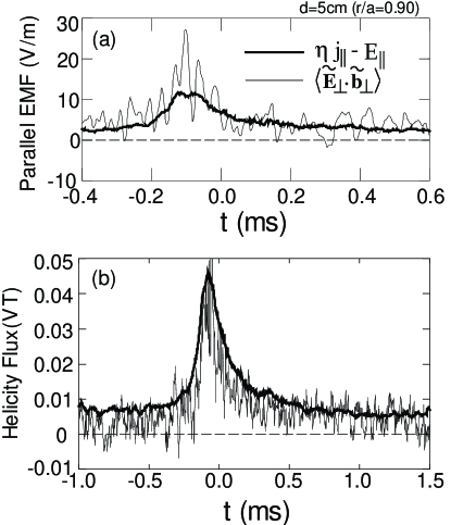
FIG. 1.: Measured (a) parallel EMF ($\alpha$-effect) due to electrostatic turbulence, $\langle\widetilde{\bf E}_{\perp}\cdot\widetilde{\bf b}_{\perp}\rangle$ (thin line) where $\widetilde{\bf E}_{\perp}=-{\mbox{\boldmath$\nabla$}}_{\perp}\widetilde{\phi}$ and ${\bf b}={\bf B}/B$, and (b) helicity flux (thin line) $\langle\widetilde{\phi}\widetilde{\bf B}\rangle$ in a laboratory plasma (Ref. 6). The thick lines in both (a) and (b) are the predictions from the rest of the terms in Ohm’s law and the helicity balance equation. The good agreements indicate that the electrostatic turbulence alone is responsible for both dynamo action and helicity transport. (The $t=0$ refers to the timing of magnetic relaxation events, during which both the $\alpha$-effect and helicity transport are enhanced over a constantly working turbulent dynamo effect.)

Despite the long history of the dynamo problem, there are no generally accepted theories on the nature of the turbulence. It also has not been investigated numerically. Experimentally, however, it has been measured that the turbulence responsible for the observed $\alpha$-effect in laboratory Reversed-Field Pinch (RFP) plasmas is predominantly electrostatic [18] or electron diamagnetic [19]. In either case, the dynamo effect causes helicity transport in the mean field without effects on the turbulent field, consistent with theories [11] and experiments [12]. Figure 1 shows an example of measured helicity flux induced by the electrostatic turbulence together with the measured $\alpha$-effect in an RFP plasma. Both measurements (thin lines) agree well with the predictions (thick lines) from the Ohm’s law and the helicity balance equation, indicating that the electrostatic turbulence alone is responsible for both dynamo action and helicity transport.

In the case of astrophysical dynamos, however, there is no observational evidence on the nature of the responsible turbulence. Such knowledge would have great implications on the role of dynamo action in helicity evolution. A good example under debate is the solar dynamo problem and its relationship with the observed twisted field lines (hence the helicity) on the solar surface [26, 27] and even in the solar wind [7]. It has been found that there is a preference in the sign of the observed helicity in each hemisphere. A generally accepted argument is that this helicity preference originates from the convection zone or even a thin layer at the bottom of the convection zone where the solar dynamo is believed to be operational [28]. If the turbulence is electromagnetic, magnetic helicity in the large-scale field will be generated while leaving the same amount of helicity with the opposite sign in the small-scale turbulence. On the other hand, if the turbulence is electrostatic or electron diamagnetic, the dynamo action will not affect helicity in the small-scale field but will transport or separate the large-scale helicity of one sign to one hemisphere while leaving the opposite helicity in the other hemisphere. After rising to the solar surface via buoyancy, these large-scale structures and its associated helicity are constantly removed from the sun by flaring. Both mechanisms can replace the lost helicity continuously. However, the former mechanism conserves magnetic helicity locally in each hemisphere while both hemispheres need to be included for the latter mechanism to conserve helicity.

Despite the lack of theoretical insight, we point out a general tendency in which the ratio of kinetic energy to magnetic energy, or the plasma beta $\beta$ in a genaral sense, may play an important role in determining the nature of the turbulence. When $\beta\lesssim 1$, the turbulence is prone to be electrostatic or electron diamagnetic, consistent with laboratory measurements. Each field line can have a different electrostatic potential $\phi$ or electron pressure $P_{e}$ insulated by the strong magnetic field, leading to notable gradients in the perpendicular direction. On the other hand, when $\beta\gg 1$, the turbulence becomes less electrostatic or electron diamagnetic due to diminishing magnetic insulation in the perpendicular direction and becomes more electromagnetic since the field lines tend to be pushed around by a much larger plasma pressure. This conjecture is supported by a general tendency of “reduction of dimensionality” [29], in which isotropic 3D turbulence reduces to anisotropic, 2D turbulence when a strong large-scale magnetic field is introduced.

In contrast to the low-beta plasmas in the laboratory, astrophysical plasmas with an active dynamo usually have a beta much larger than unity. In addition to the solar dynamo, similar situations exist for cases of the geodynamo [30] and the galactic dynamo [31, 2]. The aforementioned conjecture would predict a local conversion process of magnetic helicity by dynamo action from the turbulent field to the mean field.

Regardless of the nature of the turbulence, the total helicity is always conserved besides the resistive effects as per Eqs.(16) and (17). This can be shown more rigorously by substituting the generalized Ohm’s law Eq.(1) into the first term on the RHS of Eq.(9) to yield

$$\int{\mathchoice{{\hbox{\boldmath$\displaystyle E$}}}{{\hbox{\boldmath$\textstyle E$}}}{{\hbox{\boldmath$\scriptstyle E$}}}{{\hbox{\boldmath$\scriptscriptstyle E$}}}}\cdot{\mathchoice{{\hbox{\boldmath$\displaystyle B$}}}{{\hbox{\boldmath$\textstyle B$}}}{{\hbox{\boldmath$\scriptstyle B$}}}{{\hbox{\boldmath$\scriptscriptstyle B$}}}}dV=\int\eta{\mathchoice{{\hbox{\boldmath$\displaystyle j$}}}{{\hbox{\boldmath$\textstyle j$}}}{{\hbox{\boldmath$\scriptstyle j$}}}{{\hbox{\boldmath$\scriptscriptstyle j$}}}}\cdot{\mathchoice{{\hbox{\boldmath$\displaystyle B$}}}{{\hbox{\boldmath$\textstyle B$}}}{{\hbox{\boldmath$\scriptstyle B$}}}{{\hbox{\boldmath$\scriptscriptstyle B$}}}}dV+\int{\mbox{\boldmath$\nabla$}P_{e}\cdot{\mathchoice{{\hbox{\boldmath$\displaystyle B$}}}{{\hbox{\boldmath$\textstyle B$}}}{{\hbox{\boldmath$\scriptstyle B$}}}{{\hbox{\boldmath$\scriptscriptstyle B$}}}}\over en}dV.$$ (18)

The first term on the RHS is a resistive effect, which vanishes with zero resistivity. The second term can be rewritten as $\int(\mbox{\boldmath$\nabla$}P_{e}\cdot{\mathchoice{{\hbox{\boldmath$\displaystyle B$}}}{{\hbox{\boldmath$\textstyle B$}}}{{\hbox{\boldmath$\scriptstyle B$}}}{{\hbox{\boldmath$\scriptscriptstyle B$}}}}/en)dV=\int(T_{e}/e){\mathchoice{{\hbox{\boldmath$\displaystyle B$}}}{{\hbox{\boldmath$\textstyle B$}}}{{\hbox{\boldmath$\scriptstyle B$}}}{{\hbox{\boldmath$\scriptscriptstyle B$}}}}\cdot d{\mathchoice{{\hbox{\boldmath$\displaystyle S$}}}{{\hbox{\boldmath$\textstyle S$}}}{{\hbox{\boldmath$\scriptstyle S$}}}{{\hbox{\boldmath$\scriptscriptstyle S$}}}}+\int(T_{e}\mbox{\boldmath$\nabla$}n\cdot{\mathchoice{{\hbox{\boldmath$\displaystyle B$}}}{{\hbox{\boldmath$\textstyle B$}}}{{\hbox{\boldmath$\scriptstyle B$}}}{{\hbox{\boldmath$\scriptscriptstyle B$}}}}/en)dV=\int(T_{e}/e)(1+\ln n){\mathchoice{{\hbox{\boldmath$\displaystyle B$}}}{{\hbox{\boldmath$\textstyle B$}}}{{\hbox{\boldmath$\scriptstyle B$}}}{{\hbox{\boldmath$\scriptscriptstyle B$}}}}\cdot d{\mathchoice{{\hbox{\boldmath$\displaystyle S$}}}{{\hbox{\boldmath$\textstyle S$}}}{{\hbox{\boldmath$\scriptstyle S$}}}{{\hbox{\boldmath$\scriptscriptstyle S$}}}}-\int(\ln n\mbox{\boldmath$\nabla$}T_{e}\cdot{\mathchoice{{\hbox{\boldmath$\displaystyle B$}}}{{\hbox{\boldmath$\textstyle B$}}}{{\hbox{\boldmath$\scriptstyle B$}}}{{\hbox{\boldmath$\scriptscriptstyle B$}}}}/e)dV$ for which both finite gradients in density and electron temperature (of course also in electron pressure) along the field line are necessary conditions to change the total helicity. However, we note that such parallel gradients, especially $\nabla_{\parallel}T_{e}$, are very small owing to fast electron flow along the field lines (with a few exceptions such as in laser-produced plasmas [32]). Such effects, often called the battery effect [1], provide only a seed for magnetic field to grow in a dynamo process and, of course, it can be accompanied by small but finite magnetic helicity. The approximate conservation of the total helicity during dynamo action is consistent with laboratory observation [12].

Finally, it is worth commenting on a classical case of statistically stationary and homogeneous turbulence [5]. In this special case, by definition, all statistical quantities of the turbulence do not vary in time and space, leading to vanishing $dK_{t}/dt$ and all turbulence-induced helicity flux: terms $E$, $F$, and $G$ in Eqs.(16) and (17). It follows that from Eq.(17), term $A$ vanishes and thus only the last term in Eq.(8) survives [33]: $\mbox{\boldmath$\mathcal{E}$}\cdot\overline{\mathchoice{{\hbox{\boldmath$\displaystyle B$}}}{{\hbox{\boldmath$\textstyle B$}}}{{\hbox{\boldmath$\scriptstyle B$}}}{{\hbox{\boldmath$\scriptscriptstyle B$}}}}=-\eta\langle\widetilde{\mathchoice{{\hbox{\boldmath$\displaystyle j$}}}{{\hbox{\boldmath$\textstyle j$}}}{{\hbox{\boldmath$\scriptstyle j$}}}{{\hbox{\boldmath$\scriptscriptstyle j$}}}}\cdot\widetilde{\mathchoice{{\hbox{\boldmath$\displaystyle B$}}}{{\hbox{\boldmath$\textstyle B$}}}{{\hbox{\boldmath$\scriptstyle B$}}}{{\hbox{\boldmath$\scriptscriptstyle B$}}}}\rangle$. As a result, the $\alpha$-effect, appearing as a resistive term, generates the same amount of helicity but with opposite signs in $K_{m}$ and $K_{t}$  [13], but the helicity generation in $K_{t}$ is canceled out exactly by the resistive decay due to the turbulence, assuring $dK_{t}/dt=0$.

In summary, it has been shown that the effect of turbulent dynamos on magnetic helicity depends critically on the nature of the turbulence. When the turbulence is electromagnetic, the $\alpha$ effect converts helicity from the turbulent, small-scale field to the mean, large-scale field. On the other hand, when the turbulence is electrostatic or due to the electron diamagnetic effect, the $\alpha$ effect transports the mean-field helicity across space without dissipation. Both mechanisms can explain the observed helicity preference of large-scale magnetic structures on the solar surface but they conserve helicity in different ways. Based on laboratory observations of turbulent dynamos, it is conjectured heuristically that plasma beta plays an important role in determining the nature of the turbulence; i.e. turbulent flow is driven by (curl-free) electrostatic electric fields or electron pressure gradient when $\beta\lesssim 1$ and by (divergence-free) electromagnetic electric fields when $\beta\gg 1$. In all cases, however, dynamo processes conserve total helicity except for resistive effects and a small battery effect, consistent with the laboratory observations. Detailed understanding of dynamo turbulence and its effects on magnetic helicity await further investigations not only by theories and numerical simulations but also by observations in space and well-controlled laboratory experiments.

The author is grateful to Dr. R. Kulsrud, Dr. P. Diamond, and Dr. M. Yamada for their comments, and to Dr. S. Prager and his group for RFP data.

REFERENCES

• [1] E.N. Parker, in Cosmical Magnetic Fields (Clarendon Press, Oxford, 1979).
• [2] E.G. Zweibel and C. Heiles, Nature 385, 131 (1997).
• [3] H.K. Moffatt, Magnetic Field Generation in Electrically Conducting Fluids (Cambridge University Press, 1978)
• [4] E.N. Parker, Astro. Phys. J. 121, 293 (1955).
• [5] F. Krause and K.-H. RΓ€dler, in Mean-Field Magnetohydrodynamics and Dynamo Theory (Akademie-Verlag, Berlin, 1980).
• [6] H. Ji et al., Phys. Plasmas 3, 1935 (1996).
• [7] D.M. Rust, Geophys. Res. Lett. 21, 241 (1994).
• [8] J.B. Taylor, Rev. Mod. Phys. 58, 741 (1986).
• [9] L. Woltjer, Proc. Natl. Acad. Sci. USA 44, 489 (1958).
• [10] M.A. Berger and G.B. Field, J. Fluid Mech. 147, 133 (1984).
• [11] A.H. Boozer, J. Plasma Phys. 35, 133 (1986); E. Hameiri and A. Bhattacharjee, Phys. Fluids 30, 1743 (1987).
• [12] H. Ji, S.C. Prager, and J.S. Sarff, Phys. Rev. Lett. 74, 2945 (1995).
• [13] N. Seehafer, Phys. Rev. E 53, 1283 (1996).
• [14] A. Pouquet, U. Frish, and J. Leorat, J. Fluid Mech. 77, 321 (1976).
• [15] T. Stribling and W. H. Matthaeus, Phys. Fluids B 2, 1979 (1990).
• [16] L. Spitzer, Jr., in Physics of Fully Ionized Gases (2nd Revised Edition) (Interscience Publishers, New York, 1962).
• [17] A.V. Gruzinov and P.H. Diamond, Phys. Rev. Lett. 72, 1651 (1994); A. Bhattacharjee and Y. Yuan, Astrophys. J. 449, 739 (1995).
• [18] H. Ji et al., Phys. Rev. Lett. 73, 668 (1994).
• [19] H. Ji et al., Phys. Rev. Lett. 75, 1085 (1995).
• [20] Obviously, β€œpure electrostatic”turbulence where $\widetilde{\mathchoice{{\hbox{\boldmath$\displaystyle B$}}}{{\hbox{\boldmath$\textstyle B$}}}{{\hbox{\boldmath$\scriptstyle B$}}}{{\hbox{\boldmath$\scriptscriptstyle B$}}}}=0$ does not have dynamo effects. β€œElectrostatic”is used here to refer to the situation in which $-\langle\mbox{\boldmath$\nabla$}\widetilde{\phi}\cdot\widetilde{\mathchoice{{\hbox{\boldmath$\displaystyle B$}}}{{\hbox{\boldmath$\textstyle B$}}}{{\hbox{\boldmath$\scriptstyle B$}}}{{\hbox{\boldmath$\scriptscriptstyle B$}}}}\rangle$ dominates over all other terms in Eq.(6).
• [21] When $V$ is not singly connected or the magnetic field is not tangent to its surface, the definition of magnetic helicity needs to be modified (such as the introduction of relative helicity in Ref. 10) for gauge invariance. However, since the main conclusions do not depend on these variations, the simplest definition is used here.
• [22] J.B. Taylor and M.F. Turner, Nucl. Fusion 29, 219 (1989).
• [23] A.H. Boozer, Phys. Fluids B 5, 2271 (1993).
• [24] R.R. Mett and J.A. Tataronis, Phys. Rev. Lett. 63, 1380 (1989); J.B. Taylor, Phys. Rev. Lett. 63, 1384 (1989).
• [25] Z. Yoshida and S.M. Mahajan, Phys. Rev. Lett. 72, 3989 (1994).
• [26] D.M. Rust and A. Kumar, Solar Phys. 155, 69 (1994).
• [27] A.A. Pevtsov, R.C. Canfield, and T.R. Metcalf, Astrophys. J. 440, L109 (1995).
• [28] See, e.g. P.A. Gilman, C.A. Morrow, and E.E. DeLuca, Astrophys. J. 338, 528 (1989).
• [29] G.P. Zank and W.H. Matthaeus, Phys. Fluids A 5, 257 (1993).
• [30] See, e.g. G.A. Glatzmaier and P.H. Roberts, Science 274, 1887 (1996).
• [31] R.M. Kulsrud, Annu. Rev. Astron. Astrophys. 37 (1999) (to be published).
• [32] J. Stamper, Science 281, 1469 (1998).
• [33] N. Seehafer, Europhys. Lett. 27, 353 (1994).