TVD Scheme for the Numerical Simulation of the Axisymmetrical Selfgravitating MHD Flows

Abstract

The explicit quasi-monotonic conservative TVD scheme and numerical method for the solution of the gravitational MHD equations are developed. The 2D numerical code for the simulation of multidimensional selfgravitating MHD flows on the Eulerian cylindrical grid is constructed. The results of test calculations show that the code has a good mathematical and computational properties and can be applied to the solution of a wide class of plasma physics and astrophysics problems. We have simulated, for example, a collapse of magnetized rotating protostellar clouds.

, ,

1 Introduction

Magnetic field plays an important role in the various problems of plasma physics and astrophysics. It is well known, for example, that the density of the magnetic energy in the interstellar clouds is compared with the density of the turbulent energy and can exceed the density of the thermal energy (see, e.g., [1]). There are a wide class of problems dealing with the dynamics of the selfgravitating MHD flows. Note among others the gravitational collapse of the interstellar clouds, protostellar clusters and galaxies; origin of the molecular bipolar outflows and jets from young stars and galaxy cores; dynamics of the accretion flows and circumstellar disks.

A variety of finite-difference schemes for the solution of the gasdynamical equations have been developed during last five decades. Corresponding 1D, 2D, and 3D numerical codes have been applied to the simulation of various gasdynamical flows. The direct extension of the these schemes to the MHD, however, is quite complex problem due to the specific properties of the MHD equations (anisotropy, vanishing divergence of the magnetic field, etc.).

Among the non-monotonic generalization of gasdynamical schemes for numerical simulation of the MHD flows the Lax-Vendroff method (and its modifications) is used (see, e.g., [2]). This method is subjected to the non-physical oscillations on strong discontinuities [3]. Another prevailing method for the simulation of the multidimensional selfgravitating MHD flows is the MHD extension of the SPH method [4].

A finite-difference scheme should approximate correctly the physical oscillations of the flows containing shock waves, contact discontinuities and rarefaction waves. The nonlinear monotonic methods of high resolution were suggested for the solution of these problems. Historically the first monotonic method was FCT method [5, 6]. It was developed for of linear advection equation and for gasdynamical equations. At the present time FCT schemes are used for the simulations of the MHD flows as well [7].

There are two basic approaches that are applied for the construction of the monotonic finite-difference schemes for the numerical solution of the MHD problems. Nonlinear Riemann problem is solved in the original Godunov’s methods at every mesh interface and every time step by various iteration procedures (see, e.g., [8]). On the basis of nonlinear Riemann solver, Dai and Woodward [9] extended the PPM method [10] there. Powell et al. [11, 12] constructed an eight-wave eigensystem for the approximate Riemann solver. Jiang and Wu [13] applied a high-order WENO interpolation scheme to MHD equations. Another approach is splitting the hyperbolicity matrix onto positive and negative parts and following solution of the linear Riemann problem [14, 15, 16, 17, 18, 19, 20].

We have suggested recently a simple TVD scheme for the numerical solution of the MHD equations that has high resolution in the smooth regions of the solution (see [21]). This scheme does not demand the solution of full eigenvalues problem (i.e. a calculation of all eigenvectors and eigenvalues of the hyperbolicity matrix), since it uses only the spectral radius. On the basis of developed TVD scheme we elaborated 2D numerical method for the solution of the selfgravitational MHD equations in cylindrical coordinates [22]. This method can be used for the simulation of isothermal and adiabatic plasma flows. We have applied it to simulation of the collapse of magnetized rotating protostellar clouds.

In outline this paper proceeds as follows. In Section 2 we consider the mathematical problem statement for the simulation of selfgravitating MHD flows in the frame of axisymmetrical approximation. In Section 3 the TVD scheme for the numerical solution of the 1D MHD system is constructed. In Section 4 the developed 1D TVD scheme is extended to the 2D case and numerical algorithm for simulation of the 2D axisymmetrical selfgravitating MHD flows is described. Section 5 gives the description of 2D MHD numerical code and the results of few test problems. The results of the numerical simulations of the magnetized protostellar cloud collapse is presented in Section 6. In the conclusion (Section 7) we discuss briefly the main properties of the presented numerical code and general perspectives of its development in future.

2 Problem statement

2.1 Basic equations

The system of the gravitational MHD reads:

$$\frac{\partial\rho}{\partial t}+\nabla_{k}(\rho v^{k})=0\,,$$ (1)

$$\frac{\partial}{\partial t}\bigl{(}\rho v^{i}\bigr{)}+\nabla_{k}\bigl{(}\rho v^{i}v^{k}+g^{ik}P-\sigma^{ik}\bigr{)}=-\rho\nabla^{i}\Phi\,,$$ (2)

$$\frac{\partial B^{i}}{\partial t}-\Bigl{[}\nabla,\bigl{[}{\bf v},{\bf B}\bigr{]}\Bigr{]}^{i}=0\,,$$ (3)

$$\frac{\partial}{\partial t}\biggl{(}\rho\varepsilon+\rho\frac{{\bf v}^{2}}{2}+\frac{{\bf B}^{2}}{8\pi}\biggr{)}+\nabla_{k}\biggl{\{}\rho v^{k}\biggl{(}\varepsilon+\frac{P}{\rho}+\frac{{\bf v}^{2}}{2}\biggr{)}+\Bigl{[}{\bf B},[{\bf v},{\bf B}]\Bigr{]}^{k}\biggr{\}}$$

$$\qquad\qquad\qquad\qquad\qquad\qquad=-\rho v^{k}\nabla_{k}\Phi\,,$$ (4)

$$\nabla^{2}\Phi=4\pi G\rho\,,$$ (5)

where

$$\sigma^{ik}=\frac{B^{i}B^{k}}{4\pi}-g^{ik}\frac{{\bf B}^{2}}{8\pi}$$ (6)

is the Maxwellian tension tensor, $g^{ik}$ is the metric tensor. The other variables in this system (and further) have its usual physical sense. The system (1–6) is written in covariant form. Therefore it can be rewritten easy for the case of arbitrary curvilinear coordinates.

To close the system (1–6) we use the equation of state of a perfect gas $P=(\gamma-1)\rho\varepsilon$, where $\gamma$ is the adiabatic index. The equation of energy (4) in the case of isothermal plasma should be excluded and the pressure should be determined from the relation $P=c_{T}^{2}\rho$, $c_{T}^{2}=RT/\mu$, where $c_{T}$ is the isothermal sound speed, $\mu$ is the molecular weight.

The collapse of a rotating magnetized protostellar cloud can be studied in the frame of axisymmetric approximation if the initial uniform magnetic field ${\bf B}$ is parallel to the vector of angular velocity ${\bf\Omega}$. In this case we can use the cylindrical coordinates $(r,\varphi,z)$, axis $z$ being parallel to the vectors ${\bf B}$ and ${\bf\Omega}$. The variables in (1–6) do not depend on the azimuthal coordinate $\varphi$, so equations (1–4) can be written then in divergent form as follows:

$$\frac{\partial{\bf u}}{\partial t}+\frac{\partial{\bf F}}{\partial r}+\frac{\partial{\bf G}}{\partial z}={\bf R}\,,$$ (7)

where the vectors of the conservative variables ${\bf u}$, fluxes ${\bf F}$, ${\bf G}$ and sources ${\bf R}$ are determined by expressions:

$$\qquad\qquad{\bf u} = \left\{r\rho\,,\ r\rho v_{r}\,,\ r^{2}\rho v_{\varphi}\,,\ r\rho v_{z}\,,\ \right.$$ (8)

$$\qquad\left.B_{r}\,,\ B_{\varphi}\,,\ rB_{z}\,,\ r\left(\rho\varepsilon+\rho\frac{{\bf v}^{2}}{2}+\frac{{\bf B}^{2}}{8\pi}\right)\right\}^{T}\,,$$

$$\qquad{{\bf F}} = \left\{r\rho v_{r}\,,\ r\left(\rho v_{r}^{2}+P+\frac{{\bf B}^{2}}{8\pi}-\frac{B_{r}^{2}}{4\pi}\right)\,,\ r^{2}\left(\rho v_{r}v_{\varphi}-\frac{B_{r}B_{\varphi}}{4\pi}\right)\,,\ \right.$$ (9)

$$\qquad r\left(\rho v_{r}v_{z}-\frac{B_{r}B_{z}}{4\pi}\right)\,,\ 0\,,\ v_{r}B_{\varphi}-v_{\varphi}B_{z}\,,\ r\left(v_{r}B_{z}-v_{z}B_{r}\right)\,,$$

$$\qquad\left.r\rho v_{r}\left(\varepsilon+\frac{P}{\rho}+\frac{{\bf v}^{2}}{2}\right)+rv_{r}\frac{{\bf B}^{2}}{4\pi}-r\frac{B_{r}}{4\pi}\left({\bf v}\cdot{\bf B}\right)\right\}^{T}\,,$$

$$\qquad{\bf G} = \left\{r\rho v_{z}\,,\ r\left(\rho v_{z}v_{r}-{\displaystyle B_{z}B_{r}\over\displaystyle 4\pi}\right)\,,\ r^{2}\left(\rho v_{\varphi}v_{z}-{\displaystyle B_{\varphi}B_{z}\over\displaystyle 4\pi}\right)\,,\ \right.$$ (10)

$$\qquad r\left(\rho v_{z}^{2}+P+{\displaystyle{\bf B}^{2}\over\displaystyle 8\pi}-{\displaystyle B_{z}^{2}\over\displaystyle 4\pi}\right)\,,\ v_{z}B_{r}-v_{r}B_{z}\,,\ v_{z}B_{\varphi}-v_{\varphi}B_{z}\,,\ 0\,,\$$

$$\qquad\left.r\rho v_{z}\left(\varepsilon+{\displaystyle P\over\displaystyle\rho}+{\displaystyle{\bf v}^{2}\over\displaystyle 2}\right)+rv_{z}{\displaystyle{\bf B}^{2}\over\displaystyle 4\pi}-r{\displaystyle B_{z}\over\displaystyle 4\pi}({\bf v}\cdot{\bf B})\right\}^{T}\,,$$

$$\qquad{\bf R} = \left\{0\,,\ \rho v_{\varphi}^{2}+P+{\displaystyle{\bf B}^{2}\over\displaystyle 8\pi}-{\displaystyle B_{\varphi}^{2}\over\displaystyle 4\pi}-r\rho{\displaystyle\partial\Phi\over\displaystyle\partial r}\,,\ 0\,,\ -r\rho{\displaystyle\partial\Phi\over\displaystyle\partial z}\,,\ \right.$$ (11)

$$\qquad\left.0\,,\ 0\,,\ 0\,,\ -r\rho v_{r}{\displaystyle\partial\Phi\over\displaystyle\partial r}-r\rho v_{z}{\displaystyle\partial\Phi\over\displaystyle\partial z}\right\}^{T}\,.$$

Here index $T$ denotes the operation of the transposition.

2.2 Initial and boundary conditions

Let us consider the problem of initial and boundary condition on the example of the interstellar (protostellar) clouds collapse. Under the condition of axial and equatorial symmetries we can considered the 2D computational domain in the cylindrical coordinate system: $D=(0\leq r\leq R,0\leq z\leq Z)$ with the characteristic sizes $R$ and $Z$. We suppose that contracting cloud is located inside the computational domain and cloud boundary does not coincide with the grid boundary.

The conditions on the external boundaries of the computational domain are defined by cloud contraction from the given volume. In this case the normal components of the velocity ${\bf v}_{n}$ on the external boundary are equal to zero. For density $\rho$, internal energy $\varepsilon$, magnetic field ${\bf B}$ and tangential components of the velocity ${\bf v}_{\tau}$ we can write boundary conditions as $\partial/\partial{\bf n}=0$, where ${\bf n}$ is the outer normal unit vector. The internal boundary conditions correspond to the axial and equatorial symmetries ($v_{r}=v_{\varphi}=0$ on the axe and $\partial/\partial z=0$, $v_{z}=B_{\varphi}=B_{r}=0$ on the equator).

Initial conditions for the collapse of the rotating magnetic cloud are determined by values of the mass $M_{0}$, temperature $T_{0}$ and parameters $\epsilon_{t}$, $\epsilon_{m}$, $\epsilon_{\omega}$. These parameters are ratios of the internal, magnetic and kinetic energies of rotation to the absolute value of gravitational energy, respectively. The parameters $\epsilon_{t}$, $\epsilon_{m}$, $\epsilon_{\omega}$ allow us to obtain the following similarity relations for the variables characterizing the initial cloud state:

$$R_{0}=8.9111\cdot 10^{16}\epsilon_{t}\biggl{(}\frac{M_{0}}{M_{\odot}}\biggr{)}\biggl{(}\frac{T_{0}}{10~{}\mathrm{K}}\biggr{)}^{-1}~{}\mathrm{cm}\,,$$ (12)

$$\rho_{0}=6.7475\cdot 10^{-19}\epsilon_{t}^{-3}\biggl{(}\frac{M_{0}}{M_{\odot}}\biggr{)}^{-2}\biggl{(}\frac{T_{0}}{10~{}\mathrm{K}}\biggr{)}^{3}~{}\mathrm{g}\cdot\mathrm{cm}^{-3}\,,$$ (13)

$$\Omega_{0}=7.5204\cdot 10^{-13}\epsilon_{t}^{-3/2}\epsilon_{\omega}^{1/2}\biggl{(}\frac{M_{0}}{M_{\odot}}\biggr{)}^{-1}\biggl{(}\frac{T_{0}}{10~{}\mathrm{K}}\biggr{)}^{3/2}~{}\mathrm{s}^{-1}\,,$$ (14)

$$B_{0}=1.2342\cdot 10^{-4}\epsilon_{t}^{-2}\epsilon_{m}^{1/2}\biggl{(}\frac{M_{0}}{M_{\odot}}\biggr{)}^{-1}\biggl{(}\frac{T_{0}}{10~{}\mathrm{K}}\biggr{)}^{2}~{}\mathrm{G}\,.$$ (15)

These similarity relations allow to generalize the results of simulation with the specified values $\epsilon_{t}$, $\epsilon_{m}$, $\epsilon_{\omega}$ on the contracting clouds with other values of mass and temperature.

The minimal initial values of the parameters $\epsilon_{t}$, $\epsilon_{m}$, $\epsilon_{\omega}$ depend on the critical mass $M_{*}$. We can obtain the value of critical mass from virial theorem as follows:

$$\frac{M_{*}}{M_{0}}=\epsilon_{\omega}+\frac{3}{2}(\gamma-1)\epsilon_{t}+\sqrt{(\epsilon_{\omega}+\frac{3}{2}(\gamma-1)\epsilon_{t})^{2}+\epsilon_{m}}\,.$$

3 Finite-difference scheme

3.1 TVD schemes

Let us construct the finite-difference scheme for adiabatical and isothermal MHD flows using the total variation diminishing (TVD) principle. TVD principle for schemes approximating the linear hyperbolic system is an extension of monotonic principle for the schemes approximating the linear advection equation.

The general idea of this principle consists in the numerical implementation of the total variation diminishing for the finite-difference Riemann invariants [23]. An efficient way of the monotonic schemes construction was proposed by Vyaznikov et al. [24]. It consists in the following steps:

1. The selection of a monotonic ‘base’ scheme of the first order of approximation.

2. The transformation of the ‘base’ scheme to the high resolution scheme by addition of the antidiffusional terms.

3. The construction of the antidiffusional coefficients for monotonicity guarantee.

The constructed TVD scheme should have a high resolution in the smooth regions of the solution but the order of approximation can decrease in the regions of large gradients.

3.2 Advection equation

To investigate the general ideology of the TVD scheme construction and its basic properties let us consider the linear advection equation:

$$\frac{\partial\rho}{\partial t}+v\frac{\partial\rho}{\partial x}=0\,,\qquad\qquad v=\mathrm{const}\,,$$ (16)

that is defined in the domain $D=\{t>0$, $-\infty<x<+\infty\}$ with the initial values $\rho(x,0)=\rho_{0}(x)$. We introduce an uniform spatial grid $\{x_{i}=ih$, $i=0,\pm 1,\pm 2,\ldots\}$ with the fixed stepsize $h$ and consider the following class of ‘base’ schemes for the equation (16):

$$\frac{\rho_{i}^{n+1}-\rho_{i}^{n}}{\tau} + v\frac{\rho_{i+1}^{n}-\rho_{i-1}^{n}}{2h}-\frac{w}{2h}\bigl{(}\rho_{i+1}^{n}-2\rho_{i}^{n}+\rho_{i-1}^{n}\bigr{)}$$ (17)

$$- \frac{v-w}{4}\left(\alpha_{i+1/2}^{-}\frac{\rho_{i+1}^{n}-\rho_{i}^{n}}{h}-\alpha_{i-1/2}^{-}\frac{\rho_{i}^{n}-\rho_{i-1}^{n}}{h}\right)$$

$$+ \frac{v+w}{4}\left(\alpha_{i+1/2}^{+}\frac{\rho_{i+1}^{n}-\rho_{i}^{n}}{h}-\alpha_{i-1/2}^{+}\frac{\rho_{i}^{n}-\rho_{i-1}^{n}}{h}\right)=0\,.$$

The parameter $w$ is a coefficient of numerical viscosity, while the coefficients $\alpha_{i+1/2}\geq 0$ determine the antidiffusional terms.

If all $\alpha_{i+1/2}=0$ the scheme (17) gives the ‘base’ scheme of the first order of approximation in space and time. The condition of monotonicity of this scheme is $w\geq|v|$. In the case $w=|v|$ the ‘base’ scheme transforms into the classical donor cell scheme [25].

To obtain the conditions of monotonicity in the case of $\alpha_{i+1/2}\neq 0$ we have to use the principle of maximum [26], that for the scheme (17) gives the inequalities:

$$1-\frac{1}{2}\alpha_{i+1/2}^{-}+\frac{1}{2}\frac{\alpha_{i-1/2}^{-}}{R_{i-1/2}^{-}}\geq 0\,,\qquad\qquad\qquad$$

$$1-\frac{1}{2}\alpha_{i-1/2}^{+}+\frac{1}{2}\frac{\alpha_{i+1/2}^{+}}{R_{i+1/2}^{+}}\geq 0\,,\qquad\qquad\qquad$$ (18)

$$\frac{w-v}{2h}\tau\left(1-\frac{1}{2}\alpha_{i+1/2}^{-}+\frac{1}{2}\frac{\alpha_{i-1/2}^{-}}{R_{i-1/2}^{-}}\right)+\frac{w+v}{2h}\tau\left(1-\frac{1}{2}\alpha_{i-1/2}^{+}+\frac{1}{2}\frac{\alpha_{i+1/2}^{+}}{R_{i+1/2}^{+}}\right)$$

$$\leq 1\,,\qquad\qquad\qquad$$

where

$$R_{i+1/2}^{+}=\frac{\rho_{i}^{n}-\rho_{i-1}^{n}}{\rho_{i+1}^{n}-\rho_{i}^{n}}\,,\qquad\qquad R_{i-1/2}^{-}=\frac{\rho_{i+1}^{n}-\rho_{i}^{n}}{\rho_{i}^{n}-\rho_{i-1}^{n}}$$

are smoothness analyzers. Note that last inequality (18) determines also the stability condition for the scheme (17).

To monotonize the scheme (17) a number of approaches were suggested (see, e.g., [27, 28, 29, 30]). Vyaznikov et al. [24] proposed to consider the coefficients $\alpha$ as a piecewise-linear functions of the analyzers $R$. These functions must satisfy to the following conditions: 1) $\alpha=0$, $R\leq 0$; 2) $0\leq\alpha\leq 2$, $R\geq 0$. Let us take $\alpha(R)$ in the form of two-parametric set of piecewise-linear functions proposed by Chakravarthy and Osher [31]:

$$\alpha(R)=\frac{1+\psi}{2}\cdot\beta\cdot\mathop{\rm minmod}\nolimits(1/\beta,R)+\frac{1-\psi}{2}\cdot\mathop{\rm minmod}\nolimits(\beta,R)\,,$$

where

$$\mathop{\rm minmod}\nolimits(x,y)=\frac{1}{2}(\mathop{\rm sign}\nolimits(x)+\mathop{\rm sign}\nolimits(y))\min(|x|,|y|)\,.$$

The function $\mathop{\rm minmod}\nolimits(x,y)$ equals to zero if $x$ and $y$ have the different signs and to argument with the minimal modulus otherwise. The function $\alpha(R)$ is linear in the region of the smooth solution: $1/\beta\leq R\leq\beta$,

$$\alpha(R)=\frac{1+\psi}{2}+\frac{1-\psi}{2}R$$ (19)

and increases from value $\alpha_{1}=((1+\psi)\beta+(1-\psi))/(2\beta)$ to $\alpha_{2}=((1+\psi)+(1-\psi)\beta)/2$.

The scheme (17) has the second or third order of approximation on space in the regions of smooth solution. This result can be obtained by of expanding of the scheme (17) to the Taylor series in the neighborhood of point $M=(t=t^{n},x=x_{i})$. The corresponding first difference approximation for the scheme (17) is:

$$\frac{\partial\rho}{\partial t}+v\frac{\partial\rho}{\partial x}+\frac{v}{4}\bigl{(}\frac{1}{3}-\psi\bigr{)}\frac{\partial^{3}\rho}{\partial x^{3}}h^{2}+O(\tau+h^{3})\,,$$

Therefore at the value $\psi=1/3$ in the region of smooth solution the scheme (17) attains the third order of approximation in space. For the other values of $\psi$ the scheme (17) has the second order of approximation.

The parameters $\alpha_{1}$ and $\alpha_{2}$ determine the range of values of the function $\alpha(R)$ in the smoothness region (where $R\sim 1$). The optimal value of the parameter $\beta$ attains at $\alpha_{2}=2$ when $\beta=\beta_{max}=(3-\psi)/(1-\psi)$. In this case we can find that $\alpha_{1}=2/(3-\psi)$, $\alpha_{2}=2$. The stability condition is determined by last inequality (18). It can be rewritten in the following form:

$$\qquad\qquad\frac{w\tau}{h} + \frac{(w-v)\tau}{4h}\max\limits_{R}\left\{\frac{\alpha}{R}\right\}-\frac{(w-v)\tau}{4h}\min\limits_{R}\left\{\alpha\right\}$$

$$+ \frac{(w+v)\tau}{4h}\max\limits_{R}\left\{\frac{\alpha}{R}\right\}-\frac{(w+v)\tau}{4h}\min\limits_{R}\left\{\alpha\right\}\leq 1\,.$$

From this inequality and from the definition of $\alpha(R)$ we can obtain the stability condition of Courant, Friedrichs and Lewy (CFL condition, [32]):

$$\frac{w\tau}{h}\leq\frac{4}{5-\psi+\beta(1+\psi)}\,.$$ (20)

In the case of optimal values of the parameters $\psi=1/3$ and $\beta=4$ we can rewrite (20) by the following way:

$$\frac{w\tau}{h}\leq 0.4\,.$$

The developed scheme can be rewritten more briefly in the conservative form:

$$\frac{\rho_{i}^{n+1}-\rho_{i}^{n}}{\tau}+\frac{f_{i+1/2}-f_{i-1/2}}{h}=0\,,$$ (21)

where

$$\qquad\qquad f_{i+1/2} = f_{i+1/2}^{0}-\frac{1-\psi}{4}\mathop{\rm minmod}\nolimits(f_{i+3/2}^{-},\beta f_{i+1/2}^{-})$$ (22)

$$- \frac{1+\psi}{4}\mathop{\rm minmod}\nolimits(f_{i+1/2}^{-},\beta f_{i+3/2}^{-})$$

$$+ \frac{1+\psi}{4}\mathop{\rm minmod}\nolimits(f_{i+1/2}^{+},\beta f_{i-1/2}^{+})$$

$$+ \frac{1-\psi}{4}\mathop{\rm minmod}\nolimits(f_{i-1/2}^{+},\beta f_{i+1/2}^{+})\,,$$

$$f_{i+1/2}^{0}=\frac{f_{i+1}+f_{i}}{2}-\frac{w}{2}\left(\rho_{i+1}^{n}-\rho_{i}^{n}\right),$$

$$f_{i+1/2}^{-}=f_{i+1/2}^{0}-f_{i}\,,\qquad\qquad f_{i+1/2}^{+}=f_{i+1}-f_{i+1/2}^{0}$$

and fluxes $f_{i}=v\rho_{i}^{n}$.

3.3 System of hyperbolic equations

The developed methodology of difference scheme construction for the linear advection equation can be generalized onto the system of the linear hyperbolic equations:

$$\frac{\partial{\bf u}}{\partial t}+{\sf A}\frac{\partial{\bf u}}{\partial x}=0\,,$$ (23)

where ${\bf u}$ is the vector of the unknown variables and ${\sf A}$ is the matrix of the constant coefficients (hyperbolicity matrix). This system can be rewritten in the conservative form:

$$\frac{\partial{\bf u}}{\partial t}+\frac{\partial{\bf F}}{\partial x}=0$$

with the vector of fluxes: ${\bf F}={\sf A}{\bf u}$.

The system of equations (23) can be represented in the equivalent form of the equations for the Riemann invariants

$$S^{\alpha}=({\bf l}^{\alpha}\cdot{\bf u})$$ (24)

as

$$\frac{\partial S^{\alpha}}{\partial t}+\lambda_{\alpha}\frac{\partial S^{\alpha}}{\partial x}=0\,,$$ (25)

where ${\bf l}^{\alpha}$ are the left eigenvectors of the matrix ${\sf A}$ and $\lambda_{\alpha}$ are its eigenvalues. The original variables ${\bf u}$ can be obtained using the inverse transformation:

$${\bf u}=\sum\limits_{\alpha=1}^{N}{\bf r}_{\alpha}S^{\alpha}\,,$$ (26)

where ${\bf r}_{\alpha}$ are the right eigenvectors of the matrix ${\sf A}$.

We approximate each equation in the system (25) by the difference scheme (21):

$$\frac{S_{i}^{\alpha,n+1}-S_{i}^{\alpha,n}}{\tau}+\frac{H^{\alpha}_{i+1/2}-H^{\alpha}_{i-1/2}}{h}=0\,,$$ (27)

where fluxes

$$\qquad\qquad H^{\alpha}_{i+1/2} = H^{\alpha,0}_{i+1/2}-\frac{1-\psi}{4}\mathop{\rm minmod}\nolimits(H^{\alpha-}_{i+3/2},\beta H^{\alpha-}_{i+1/2})$$

$$- \frac{1+\psi}{4}\mathop{\rm minmod}\nolimits(H^{\alpha-}_{i+1/2},\beta H^{\alpha-}_{i+3/2})$$

$$+ \frac{1+\psi}{4}\mathop{\rm minmod}\nolimits(H^{\alpha+}_{i+1/2},\beta H^{\alpha+}_{i-1/2})$$

$$+ \frac{1-\psi}{4}\mathop{\rm minmod}\nolimits(H^{\alpha+}_{i-1/2},\beta H^{\alpha+}_{i+1/2})\,,$$

$$H^{\alpha,0}_{i+1/2}=\frac{H^{\alpha}_{i+1}+H^{\alpha}_{i}}{2}-\frac{w_{\alpha}}{2}\left(S^{\alpha,n}_{i+1}-S^{\alpha,n}_{i}\right)\,,\ \ H^{\alpha}_{i}=\lambda_{\alpha}S^{\alpha,n}_{i}\,,\ \ w_{\alpha}\geq|\lambda_{\alpha}|\,,$$

$$H^{\alpha-}_{i+1/2}=H^{\alpha,0}_{i+1/2}-H^{\alpha}_{i}\,,\ \ H^{\alpha+}_{i+1/2}=H^{\alpha}_{i+1}-H^{\alpha,0}_{i+1/2}\,.$$

To construct the scheme for the variables ${\bf u}$ we have to perform the transformation (24) in (27). Finally the scheme reads:

$$\frac{{\bf u}^{n+1}_{i}-{\bf u}^{n}_{i}}{\tau}+\frac{{\bf F}_{i+1/2}-{\bf F}_{i-1/2}}{h}=0\,,$$ (28)

where fluxes are:

$$\qquad\qquad{\bf F}_{i+1/2} = {\bf F}^{0}_{i+1/2}-\frac{1-\psi}{4}\sum\limits_{\alpha}\mathop{\rm minmod}\nolimits({\bf F}^{\alpha-}_{i+3/2},\beta{\bf F}^{\alpha-}_{i+1/2})$$ (29)

$$- \frac{1+\psi}{4}\sum\limits_{\alpha}\mathop{\rm minmod}\nolimits({\bf F}^{\alpha-}_{i+1/2},\beta{\bf F}^{\alpha-}_{i+3/2})$$

$$+ \frac{1+\psi}{4}\sum\limits_{\alpha}\mathop{\rm minmod}\nolimits({\bf F}^{\alpha+}_{i+1/2},\beta{\bf F}^{\alpha+}_{i-1/2})$$

$$+ \frac{1-\psi}{4}\sum\limits_{\alpha}\mathop{\rm minmod}\nolimits({\bf F}^{\alpha+}_{i-1/2},\beta{\bf F}^{\alpha+}_{i+1/2})\,,$$

$${\bf F}^{0}_{i+1/2}=\frac{{\bf F}_{i+1}+{\bf F}_{i}}{2}-\frac{1}{2}{\sf R}{\sf W}{\sf L}\left({\bf u}^{n}_{i+1}-{\bf u}^{n}_{i}\right)\,,$$

$${\sf W}={\mathop{\rm diag}\nolimits}(w_{1},w_{2},\ldots,w_{N})\,,$$

$${\bf F}^{\alpha\pm}_{i+1/2}=\frac{1}{2}\left(\lambda_{\alpha}\pm w_{\alpha}\right)\left({\bf l}_{\alpha}\cdot\left({\bf u}^{n}_{i+1}-{\bf u}^{n}_{i}\right)\right){\bf r}^{\alpha}\,,$$

where ${\sf L}$, ${\sf R}$ – matrixes of the left and of the right eigenvectors of the matrix ${\sf A}$ respectively.

The difference scheme (28,29) satisfies to the total variation diminishing (TVD) principle [23], since it is constructed on the basis of the monotonic schemes for the Riemann invariants. In the present paper we consider the Lax–Friedrichs schemes with the coefficients $w_{\alpha}=w\geq\max\limits_{\alpha}\{|\lambda_{\alpha}|\}$. For this case the fluxes in the base scheme reads [33, 34]:

$${\bf F}^{0}_{i+1/2}=\frac{{\bf F}_{i+1}+{\bf F}_{i}}{2}-\frac{w}{2}\left({\bf u}^{n}_{i+1}-{\bf u}^{n}_{i}\right)\,.$$ (30)

During the calculation of fluxes (29) the numerical procedure of the $\mathop{\rm minmod}\nolimits$-evaluation should be called very often. To decrease the computation time we consider a more simple scheme in which the additional fluxes are summed up. Finally the scheme (28) is determined by the fluxes:

$$\qquad\qquad{\bf F}_{i+1/2} = {\bf F}^{0}_{i+1/2}-\frac{1-\psi}{4}\mathop{\rm minmod}\nolimits({\bf F}^{-}_{i+3/2},\beta{\bf F}^{-}_{i+1/2})$$ (31)

$$- \frac{1+\psi}{4}\mathop{\rm minmod}\nolimits({\bf F}^{-}_{i+1/2},\beta{\bf F}^{-}_{i+3/2})$$

$$+ \frac{1+\psi}{4}\mathop{\rm minmod}\nolimits({\bf F}^{+}_{i+1/2},\beta{\bf F}^{+}_{i-1/2})$$

$$+ \frac{1-\psi}{4}\mathop{\rm minmod}\nolimits({\bf F}^{+}_{i-1/2},\beta{\bf F}^{+}_{i+1/2})\,,$$

where

$${\bf F}^{-}_{i+1/2}={\bf F}^{0}_{i+1/2}-{\bf F}_{i},\qquad\qquad{\bf F}^{+}_{i+1/2}={\bf F}_{i+1}-{\bf F}^{0}_{i+1/2}$$

and the fluxes ${\bf F}^{0}_{i+1/2}$ are determined by the expression (30).

This methodology can be generalized easy onto the system of the nonlinear equations:

$$\frac{\partial{\bf u}}{\partial t}+\frac{\partial{\bf F}({\bf u})}{\partial x}=0\,.$$ (32)

The finite-difference scheme (28) for the system (32) is determined by the same fluxes (30,31), but the coefficients $w$ we should take in the form:

$$w=w_{i+1/2}=\phi\max\limits_{\alpha}\left\{|\lambda_{\alpha,i}|,|\lambda_{\alpha,i+1}|\right\}\,,\ \ \phi\geq 1\,,$$ (33)

where $\lambda_{\alpha}$ are the eigenvalues of the hyperbolicity matrix ${\sf A}=\partial{\bf F}/\partial{\bf u}$.

3.4 MHD modification of the finite-difference scheme

We construct now the finite-difference TVD scheme for the isothermal or adiabatical 1D MHD in Cartesian coordinates. We assume that the magnetic field and the velocity have all three components: ${\bf B}=\{B_{x},B_{y},B_{z}\}$, ${\bf v}=\{v_{x},v_{y},v_{z}\}$.

The MHD equations in the conservative form,

$$\frac{\partial{\bf u}}{\partial t}+\frac{\partial{\bf F}}{\partial x}=0$$

are determined by the vector of the conservative variables:

$${\bf u}=\left\{\rho\,,\ \rho v_{x}\,,\ \rho v_{y}\,,\ \rho v_{z}\,,\ B_{x}\,,\ B_{y}\,,\ B_{z}\,,\ \rho\varepsilon+\rho\frac{{\bf v}^{2}}{2}+\frac{{\bf B}^{2}}{8\pi}\right\}^{T}$$

and by the vector of the fluxes:

$${{\bf F}} = \left\{\rho v_{x}\,,\ P+\rho v_{x}^{2}+\frac{{\bf B}^{2}}{8\pi}-\frac{B_{x}^{2}}{4\pi}\,,\ \rho v_{x}v_{y}-\frac{B_{x}B_{y}}{4\pi}\,,\ \rho v_{x}v_{z}-\frac{B_{x}B_{z}}{4\pi}\,,\ \right.$$

$$\qquad\qquad 0\,,\ v_{x}B_{y}-v_{y}B_{x}\,,\ v_{x}B_{z}-v_{z}B_{x}\,,\$$

$$\qquad\qquad\left.\rho v_{x}\left(\varepsilon+\frac{P}{\rho}+\frac{{\bf v}^{2}}{2}+\frac{{\bf B}^{2}}{4\pi}\right)-\frac{B_{x}}{4\pi}\left(v_{x}B_{x}+v_{y}B_{y}+v_{z}B_{z}\right)\right\}^{T}\,.$$

For the adiabatic case the hyperbolicity matrix ${\sf A}$ is

$$\left(\begin{array}[]{cccccccc}0&1&0&0&0&0&0&0\\ {}\hfil\\ A_{21}&(3-\gamma)v_{x}&(1-\gamma)v_{y}&(1-\gamma)v_{z}&-\gamma{\displaystyle B_{x}\over\displaystyle 4\pi}&A_{26}&A_{27}&\gamma-1\\ {}\hfil\\ -v_{x}v_{y}&v_{y}&v_{x}&0&-{\displaystyle B_{y}\over\displaystyle 4\pi}&-{\displaystyle B_{x}\over\displaystyle 4\pi}&0&0\\ {}\hfil\\ -v_{x}v_{z}&v_{z}&0&v_{x}&-{\displaystyle B_{z}\over\displaystyle 4\pi}&0&-{\displaystyle B_{x}\over\displaystyle 4\pi}&0\\ {}\hfil\\ 0&0&0&0&0&0&0&0\\ {}\hfil\\ A_{61}&{\displaystyle B_{y}\over\displaystyle\rho}&-{\displaystyle B_{x}\over\displaystyle\rho}&0&-v_{y}&v_{x}&0&0\\ {}\hfil\\ A_{71}&{\displaystyle B_{z}\over\displaystyle\rho}&0&-{\displaystyle B_{x}\over\displaystyle\rho}&-v_{z}&0&v_{x}&0\\ {}\hfil\\ A_{81}&A_{82}&A_{83}&A_{84}&A_{85}&A_{86}&A_{87}&\gamma v_{x}\end{array}\right)$$ (34)

where:

$$A_{21}=\frac{\gamma-1}{2}{\bf v}^{2}-v_{x}^{2}\,,\qquad A_{26}=(2-\gamma)\frac{B_{y}}{4\pi}\,,\qquad A_{27}=(2-\gamma)\frac{B_{z}}{4\pi}\,,$$

$$A_{61}=\frac{v_{y}B_{x}-v_{x}B_{y}}{\rho}\,,\qquad A_{71}=\frac{v_{z}B_{x}-v_{x}B_{z}}{\rho}\,,$$

$$A_{81}=-v_{x}\left(\frac{c^{2}}{\gamma-1}+\left(1-\frac{\gamma}{2}\right){\bf v}^{2}+{\bf a}^{2}\right)+a_{x}({\bf a}\cdot{\bf v})\,,$$

$$A_{82}=\frac{c^{2}}{\gamma-1}+\frac{{\bf v}^{2}}{2}+{\bf a}^{2}-a_{x}^{2}-(\gamma-1)v_{x}^{2}\,,$$

$$A_{83}=(1-\gamma)v_{x}v_{y}-a_{x}a_{y}\,,\ \ A_{84}=(1-\gamma)v_{x}v_{z}-a_{x}a_{z}\,,$$

$$A_{85}=-\gamma v_{x}\frac{B_{x}}{4\pi}-v_{y}\frac{B_{y}}{4\pi}-v_{z}\frac{B_{z}}{4\pi}\,,\qquad A_{86}=-\gamma v_{x}\frac{B_{y}}{4\pi}+v_{x}\frac{B_{y}}{2\pi}-v_{y}\frac{B_{x}}{2\pi}\,,$$

$$A_{87}=-\gamma v_{x}\frac{B_{z}}{4\pi}+v_{x}\frac{B_{z}}{2\pi}-v_{z}\frac{B_{x}}{2\pi}\,.$$

We use here the sound speed, $c=\sqrt{\gamma P/\rho}$ and ${\bf a}={\bf B}/\sqrt{4\pi\rho}$. The calculations give the following expressions for the eigenvalues of the hyperbolicity matrix (34):

$$\lambda_{1}=0\,,\ \ \lambda_{2}=v_{x}\,,\ \ \lambda_{3,4}=v_{x}\pm a_{x}\,,$$

$$\lambda_{5,6,7,8}=v_{x}\pm\sqrt{\frac{c^{2}+{\bf a}^{2}}{2}\pm\frac{1}{2}\sqrt{(c^{2}+{\bf a}^{2})^{2}-4a_{x}^{2}c^{2}}}.$$ (35)

The zero value of $\lambda_{1}$ is the consequence of zero value of the flux ${\bf F}$ component corresponding to $B_{x}$. The value of $\lambda_{2}$ corresponds to the entropic wave, $\lambda_{3,4}$ correspond to the Alfvén waves, and $\lambda_{5,6,7,8}$ correspond to the fast and slow magnetosonic waves. In the isothermal case the entropic wave disappears and instead adiabatical sound speed it should be used the isothermal sound speed $c_{T}$.

We should construct now the calculation rule for the coefficients $w$ in (33). The values of these coefficients should be not less than the maximal modulus of all eigenvalues of the hyperbolicity matrix. It is clear that this condition can be satisfied by the following way:

$$w_{i+1/2}=\phi\max\{|v_{x,i}|+\Psi_{x,i}\,,|v_{x,i+1}|+\Psi_{x,i+1}\}\,,\ \ \phi\geq 1\,,$$ (36)

where

$$\Psi_{x}=\sqrt{\frac{c^{2}+{\bf a}^{2}}{2}+\frac{1}{2}\sqrt{(c^{2}+{\bf a}^{2})^{2}-4a_{x}^{2}c^{2}}}\,.$$

Therefore we can keep in the relation (33) only eigenvalues corresponding to the fast MHD waves. This allow us to adapt the scheme (28,30,31,36) to the simulation of the 1D MHD flows. If the magnetic field is absent the fast magnetosonic speed $\Psi_{x}$ equals the sound speed $c$, therefore the transition to the gasdynamics occurs correctly. With the help of the splitting technique we can construct the scheme for multidimensional (2D and 3D) MHD flows. One of this scheme for the axisymmetric case we will describe in the next section.

4 Numerical method

4.1 General scheme

The computational grid is determined by points $(r_{i},z_{j})$ indexed by integer indexes $i=0,1,\ldots,I$; $j=0,1,\ldots,J$. These points denote the centers of the grid cells. The coordinates of the cell boundaries are defined as the arithmetic mean of corresponding coordinates of the cell centers and have half-integer indexes. The computational variables are related to the centers of the cells and the numerical fluxes are related to the cell boundaries. Above we developed the TVD scheme in the frame of 1D MHD approximation. Now we generalize this approach onto the 2D MHD approximation. The ‘base’ difference scheme for equations (7) is the following one:

$$\frac{{\bf u}_{i,j}^{n+1}-{\bf u}_{i,j}^{n}}{\triangle t}+\frac{{\bf F}_{i+1/2,j}-{\bf F}_{i-1/2,j}}{\triangle r}+\frac{{\bf G}_{i,j+1/2}-{\bf G}_{i,j-1/2}}{\triangle z}={\bf R}_{i,j}\,.$$

The main problem here is the definition of the calculation rule for the numerical fluxes across the cell boundaries.

Let us consider for simplicity only the radial direction because of the expressions of fluxes for the vertical direction can be derived by similar way. The radial fluxes ${\bf F}_{i+1/2,j}$ and ${\bf F}_{i-1/2,j}$ should be calculated with the help of the formulae (30,31,33). Relatively determination of the coefficients $w$ we should note the following.

In the definition of the vectors ${\bf u}$, ${\bf F}$ and ${\bf G}$ in the form (8–10) the radial coordinate $r$ is present. Therefore to calculate eigenvalues of the hyperbolicity matrices we can close formally the system (7) by the following obvious equation:

$$\frac{\partial r}{\partial t}=0\,.$$

It can be shown that this extension of the original MHD system not changes the standard set of the eigenvalues.

In fact we consider the following system of MHD equations:

$$\frac{\partial{\bf w}}{\partial t}+{\sf A}\frac{\partial{\bf w}}{\partial r}+{\sf B}\frac{\partial{\bf w}}{\partial z}={\bf R}\,,$$ (37)

with the vector ${\bf w}$ determined as

$${\bf w}=\left\{r\,,\ \rho\,,\ \rho v_{r}\,,\ \rho v_{\varphi}\,,\ \rho v_{z}\,,\ B_{r}\,,\ B_{\varphi}\,,\ B_{z}\,,\ \rho\left(\varepsilon+\frac{{\bf v}^{2}}{2}\right)+\frac{{\bf B}^{2}}{8\pi}\right\}^{T}\,.$$

Obviously in Cartesian coordinates the eigenvalues of matrices ${\sf A}$ and ${\sf B}$ are determined by the same expressions (35). Let us consider another vector of the variables ${\bf u}$ that consists of $r$ and eight components of the vector (8). Making the transformation of the equation (37) to the new variables ${\bf u}$ we obtain:

$$\frac{\partial{\bf u}}{\partial t}+{\sf A}^{\prime}\frac{\partial{\bf u}}{\partial r}+{\sf B}^{\prime}\frac{\partial{\bf u}}{\partial z}={\bf R}^{\prime}\,,$$

where

$${\sf A}^{\prime}={\sf T}^{-1}{\sf A}{\sf T}\,,\qquad{\sf B}^{\prime}={\sf T}^{-1}{\sf B}{\sf T}\,,\qquad{\bf R}^{\prime}={\sf T}^{-1}{\bf R}\,,$$ (38)

and matrix ${\sf T}=\partial{\bf u}/\partial{\bf w}$ is Jacobian of transformation. The determinant of this matrix $\det\hat{\sf T}=1/r^{7}$ is not equal to zero. Hence the formulae (38) describes the similarity transformations of matrices ${\sf A}$ and ${\sf B}$ that does not change their eigenvalues.

This discussion allows us to take the values of the coefficients $w_{i+1/2}$ in (33) in the following form:

$$w_{i+1/2}=\phi\max\{|v_{r,i}|+\Psi_{r,i}\,,|v_{r,i+1}|+\Psi_{r,i+1}\},\,\qquad\phi\geq 1\,,$$ (39)

where

$$\Psi_{r}=\sqrt{\frac{c^{2}+{\bf a}^{2}+\sqrt{(c^{2}+{\bf a}^{2})^{2}-4a_{r}^{2}c^{2}}}{2}}\,.$$ (40)

These coefficients are determined by eigenvalues that correspond to the fast magnetosonic wave. The expressions (39) can be applied both to the adiabatical and to the isothermal plasma flows. The energy equation should be excluded in last case and as $c$ in (40) should be used the isothermal sound speed $c_{T}$.

Since the fluxes related to the different space directions are constructed independently, the $z$-part of the numerical scheme can be developed by similar way.

4.2 Poisson solver

Poisson equation for the gravitational potential is solved by ADI-method (alternating directions implicit method) of Douglas and Rachford [35, 36, 37]:

$$\frac{\bar{\Phi}-\Phi^{p}}{\tau_{p}}=\theta\Lambda_{rr}\bar{\Phi}+(1-\theta)\Lambda_{zz}\Phi^{p}-\frac{\rho}{2}$$

$$\frac{\Phi^{p+1}-\bar{\Phi}}{\tau_{p}}=(1-\theta)\Lambda_{rr}\bar{\Phi}+\theta\Lambda_{zz}\Phi^{p+1}-\frac{\rho}{2}$$

where $\theta$ is the parameter of scheme implicity, $\Lambda_{rr}$, $\Lambda_{zz}$ are second order finite-difference approximations of the corresponding parts of Laplacian operator in $r$– and $z$–directions, respectively, $\tau_{p}$ is the iteration parameter.

Boundary conditions for the gravitational potential on the inner boundaries are regular: $\partial\Phi/\partial{\bf n}=0$. Boundary condition on the external boundary is $\Phi_{int}=\Phi_{ext}$ where $\Phi_{int}$ is the computing potential, $\Phi_{ext}$ is the external potential of the protostellar cloud. It can be obtained from Poisson integral transformation of equation (5) solution:

$$\Phi_{ext}(r,z)=-G\sum\limits_{l=0}^{\infty}\frac{P_{l}(x)}{(r^{2}+z^{2})^{l+1}/2}\int\limits_{V^{\prime}}{\d}V^{\prime}\rho(r^{\prime},z^{\prime})(r^{\prime 2}+z^{\prime 2})^{l/2}P_{l}(x^{\prime})\,,$$

where $x=z(r^{2}+z^{2})^{-l/2}$, and $P_{l}(x)$ is the Legendre polynomial of $l$th order. All terms with odd $l$ are absent in this representation as a result of the axial symmetry.

4.3 Implementation of the $\mathop{\rm div}\nolimits{\bf B}=0$ condition

Another difficulty of the numerical simulation of the multidimensional MHD flows is connected with the necessity of the numerical implementation of the vanishing divergence condition for the magnetic field

$$\mathop{\rm div}\nolimits{\bf B}=0\,.$$ (41)

Numerical errors due to discretization and finite-difference differential operator splitting can lead to nonzero divergence over the time. This problem can be solved by many ways [38]. In the first approach the 8-wave formulation of the MHD equations is used (see also [11]). Another way uses the constrained transport suggested by Evans and Hawley [39]. Finally, the third approach is the projection scheme [40]. Our numerical scheme uses the last method (see [18, 41]).

Denote as ${\bf B}^{*}$ the magnetic field obtained by the numerical solution of the induction equation (3). This ‘numerical’ magnetic field contains the numerical error ${\bf b}$, that consist of vortex and potential parts:

$${\bf b}=[\nabla,{\bf a}]+\nabla\phi\,.$$

Therefore exact solution of induction equation is:

$${\bf B}={\bf B}^{*}-{\bf b}\,.$$ (42)

Vortex part of numerical error $[\nabla,{\bf a}]$ does not contributes to divergence of the magnetic field ${\bf B}$. Substitution of (42) into (41) shows that potential $\phi$ must satisfy the Poisson equation

$$\nabla^{2}\phi=\mathop{\rm div}\nolimits{\bf B}^{*}\,.$$ (43)

Resolving this equation numerically for the defined ‘numerical’ magnetic field ${\bf B}^{*}$ for each time step we calculate the divergence free magnetic field with the help of formula

$${\bf B}^{s}={\bf B}^{*}-\nabla\phi\,.$$

Further we will assume that ${\bf B}={\bf B}^{s}$. The algorithm is implemented in our numerical code as follows. Denote the central cell with indexes ($i$, $j$) by the index $C$ for brevity (see. Fig. 1), the neighbor cells by indexes $W$, $N$, $E$, $S$ and intermediate coordinates (cell boundaries) by double indexes $CE$, $CS$ etc.

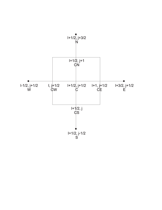
Figure 1: A typical grid cell

Then we can approximate the divergence of magnetic field by the expression:

$$\bigl{(}\mathop{\rm div}\nolimits{{\bf B}}\bigr{)}_{C}=\frac{1}{r_{C}}\frac{r_{CE}B_{r,CE}-r_{CW}B_{r,CW}}{r_{CE}-r_{CW}}+\frac{B_{z,CN}-B_{z,CS}}{z_{CN}-z_{CS}}\,,$$ (44)

where intermediate values are calculated by the formulae

$$B_{r,CE}=\frac{1}{2}\bigl{(}B_{r,C}+B_{r,E}\bigr{)}\,,\qquad B_{r,CS}=\frac{1}{2}\bigl{(}B_{r,C}+B_{r,S}\bigr{)}\,,\qquad\mathrm{etc.}$$

The finite-difference approximation of the Laplacian operator is

$$\qquad\qquad\bigl{(}\triangle\phi\bigr{)}_{C} = \frac{1}{r_{C}(r_{CE}-r_{CW})}\biggl{(}r_{CE}\frac{\phi_{E}-\phi_{C}}{r_{E}-r_{C}}-r_{CW}\frac{\phi_{C}-\phi_{W}}{r_{C}-r_{W}}\biggr{)}$$

$$+ \frac{1}{(z_{CN}-r_{CS})}\biggl{(}\frac{\phi_{N}-\phi_{C}}{z_{N}-z_{C}}-\frac{\phi_{C}-\phi_{S}}{z_{C}-z_{S}}\biggr{)}\,.$$

It is easy to see that if the potential $\phi$ is the exact solution of the finite-difference Poisson equation (43) then the magnetic field ${\bf B}$ (for which the finite-difference divergence (44) is equal to zero exactly) can be obtained by the formulae:

$$B_{r,C}=B^{*}_{r,C}-\frac{1}{2}\biggl{[}\frac{\phi_{E}-\phi_{C}}{r_{E}-r_{C}}+\frac{\phi_{C}-\phi_{W}}{r_{C}-r_{W}}\biggr{]}\,,$$

$$B_{z,C}=B^{*}_{z,C}-\frac{1}{2}\biggl{[}\frac{\phi_{N}-\phi_{C}}{z_{N}-z_{C}}+\frac{\phi_{C}-\phi_{S}}{z_{C}-z_{S}}\biggr{]}\,.$$

The Poisson equation (43) for the potential $\phi$ is solved in our scheme by the ADI-method that is described in the previous section. As the additional boundary conditions on the inner boundaries ($r=0$, $z=0$) we use the relations $\partial\phi/\partial{\bf n}=0$. On the outer boundaries we use the boundary condition $\phi=0$ since the external field has identically vanishing divergence.

5 Test computations

5.1 Background

The numerical code ‘Moon’ was developed on the basis of the proposed finite-difference scheme. It can simulate the 1D and 2D selfgravitating MHD flows. The code is implemented by the programming language C++ and completely object-oriented. Source text of the program uses only standard C++ elements and does not relate to concrete compiler. The kernel of the code uses intensively the object-oriented library ‘Numerical Tool Box’ (NTB 3.5). This library was developed by A.G.Zhilkin in 1996 for more easy creation of the complex numerical codes. To check the properties of our code we tested it on the number of test problems with known (exact or approximate) analytical solutions.

5.2 One-dimensional tests

5.2.1 Test 1. Linear advection

The linear advection of the square density profile was simulated to check the phase-error properties of the numerical scheme. Figure 2 gives the density profile after 100th time step without (triangles) and with flux correction (dots). The computational grid consists of 100 cells. The analytical solution is drawn by the solid line.

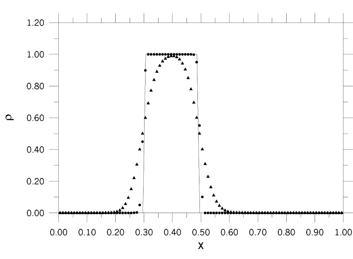
Figure 2: Linear advection of squared density profile. The density distributions is shown after 100 time-step computed by the scheme of the 1st-order of approximation (triangles) and by the scheme of the 3rd-order of approximation (dots). The solid line corresponds to the analytical solution

It is seen that the 1st-order of approximation method has a large numerical diffusion. This diffusion smears the initial profile rapidly, the width of smearing being increased during calculation. The method of the 3rd-order of approximation produces a profile that is smeared onto 3–4 cells only and conserves its form during a long time. We can say therefore that amplitude and phase errors in the scheme of the 3rd-order of approximation are selfconsistent and its order of approximation is not less actually then the approximation order of the so-called LPE-schemes (little phase error) (see [6]). In our opinion this circumstance is connected with the successful selection of the antidiffusion limiters (22) in the scheme (21).

5.2.2 Test 2. Decay of arbitrary gasdynamical discontinuity

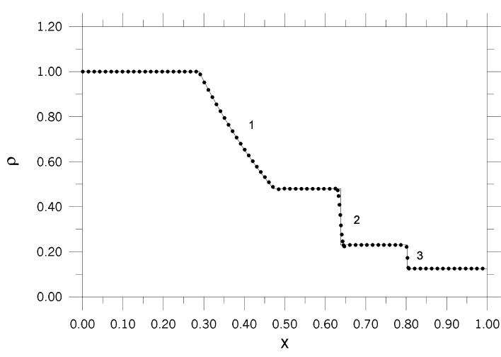
Figure 3: Decay of an gasdynamical discontinuity. The density distribution (dots) is shown at the time moment $t=0.164$. The solid line corresponds to the analytical solution. The digits correspond to: 1 — rarefaction wave, 2 — contact discontinuity, 3 — shock wave. In the regions of smooth flow the dots is displayed more seldom (each 7th point). In the regions of contact discontinuity and shock wave all points of numerical solution are displayed

Numerical simulation of the arbitrary discontinuity decay (Riemann problem) allows us to check the scheme properties relating to the resolution of the shock waves, contact discontinuities and rarefaction waves. At the initial time moment the computational domain along the $x$-axis was divided on two subdomains $A$ and $B$. In the initial state the pressure and density have the following values: in subdomain $A$ — $\rho_{A}=1$, $P_{A}=1$; in subdomain $B$ — $\rho_{B}=0.125$, $P_{B}=0.1$. The velocity in both domains $v_{A}=v_{B}=0$ and adiabatic index $\gamma=5/3$. Figure 3 shows the analytical solution (solid line) and the results of the numerical computation (dots) at the time moment $t=0.164$. As a result of the discontinuity decay the rarefaction wave 1 propagates to the left, contact discontinuity 2 and shock wave 3 propagates to the right. The Figure shows that the scheme resolves the shock wave sufficiently well, but gives the small non-physical oscillations on the contact discontinuity. To smooth it is necessary to use additional limiters of antidiffusion fluxes.

  

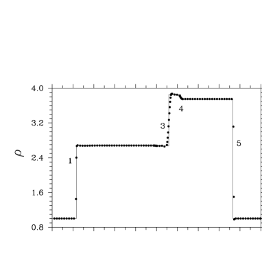
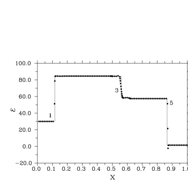
Figure 4: Decay of an MHD discontinuity (variant 1). The solution is corresponded to time moment $t=0.08$. The digits correspond to: 1,5 — fast MHD shock waves, 2 — rotational (alfvenic) discontinuity, 3 — contact discontinuity, 4 — slow MHD shock wave

5.2.3 Tests 3, 4. Decay of arbitrary MHD discontinuity

The numerical simulation of an arbitrary MHD discontinuity decay is the unique possibility to check the MHD properties of the difference scheme. The problem statement in this test is similar to the problem statement in test 2. The initial parameters for this test and its exact analytical solution were taken from paper of Ryu and Jones [18] (variant 1a): $\gamma=5/3$, $\rho_{A}=1$, $\rho_{B}=1$, $P_{A}=20$, $P_{B}=1$, $v_{x,A}=10$, $v_{x,B}=-10$, $B_{y,A}=5$, $B_{y,B}=5$, $B_{x}=5$. The values of another variables are taken to be zero. This situation can arise, for example, at the collision of two gaseous masses moving forward each to other at the angle $\pi/4$ to the direction of the magnetic field.

The results of the numerical computation and the analytical solution of this problem at the time $t=0.08$ are shown on the Fig. 4. As a result of the discontinuity decay two fast MHD shock waves (1 and 5) arise and propagate in the opposite directions. The rotational (alfvenic) discontinuity 2, the contact discontinuity 3 and the slow MHD shock wave 4 are formed between this waves. The slow MHD shock wave propagates immediately after the fast MHD shock wave to the region of the gas with the larger pressure.

  

  

Figure 5: Decay of an MHD discontinuity (variant 2). The solution is corresponded to time moment $t=0.15$. The digits correspond to: 1 — fast MHD shock wave, 2 — slow MHD shock wave, 3 — contact discontinuity, 4 — gasdynamical shock wave

In another variant of this test we consider the Riemann problem with the initial state vector $(\rho,v_{x},v_{y},v_{z},B_{y},B_{z},P)$ (see [18], variant 4c): region $A$ — $(0.65,0.667,-0.257,0,0.55,0,0.5)$, region $B$ — $(1,0.4,-0.94,0,0,0,0.75)$ with $B_{x}=0.75$ and $\gamma=5/3$. The switch-of slow shock wave is formed in this case. The results of computations at the time $t=0.15$ are shown on Fig. 5. A fast MHD shock wave 1, switch-of slow MHD shock wave 2, contact discontinuity 3 and gasdynamical shock wave 4 are formed.

These tests show that the scheme approximation of fast and slow shock waves as well as the rotational (alfvenic) discontinuity is good enough. On the contact discontinuities and on the switch-off shock wave small oscillations occur.

5.2.4 Test 5. Alfvén wave

The problem of propagation of the finite amplitude Alfvén wave (the simple alfvenic wave) is interesting because it has the analytical solution (see [42]). The comparison of the numerical and the analytical velocity profiles and the magnetic field allows us to make conclusions about behavior of the phase and the amplitude errors in the MHD case. We solve the following problem. At the initial time moment the wave is concentrated in the region $x_{L}\leq x\leq x_{R}$, where

$$B_{y}=10\sin\left(\pi\frac{x_{R}-x}{x_{R}-x_{L}}-\frac{\pi}{2}\right)\,,\ \ B_{z}=10\cos\left(\pi\frac{x_{R}-x}{x_{R}-x_{L}}-\frac{\pi}{2}\right)\,,$$

$$v_{y}=\frac{B_{y}}{\sqrt{4\pi\rho}},\qquad\qquad v_{z}=\frac{B_{z}}{\sqrt{4\pi\rho}}\,.$$

The wave propagates in the gas with parameters $\rho=1$, $P=1$, $v_{x}=0$, $B_{x}=1$, $\gamma=1.4$ with velocity $a=B_{x}/\sqrt{4\pi\rho}$ without profile distortion. In wave region the tangential component of the magnetic field rotates with the conservation of its absolute value. Figure 6. shows the numerical and analytical distributions $B_{y}$ and $B_{z}$ at the time moment $t=0.3$.

The comparison of these curves with each other allows us to make the conclusion that even in the case of full MHD system the essential smearing of the velocity and the magnetic field profiles is absent during a sufficiently long time of the computation. Hence the phase errors balance the amplitude ones with the high order of accuracy.

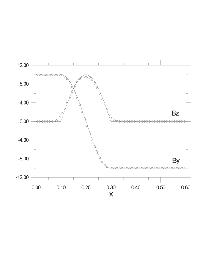
Figure 6: Alfvén wave. The numerical (circles) and the analytical (solid lines) distributions of the transverse components of the magnetic field are shown at the time moment $t=0.3$

5.3 Two-dimensional tests

5.3.1 Test 6. Two-dimensional advection

To check the diffusion properties of the developed 2D code we obtain the numerical solution of the 2D advection equation (see similar computations of Munz [43])

$$\frac{\partial\rho}{\partial t}+v_{x}(y)\frac{\partial\rho}{\partial x}+v_{y}(x)\frac{\partial\rho}{\partial y}=0$$

in box domain $(0\leq x,y\leq 1)$. The analytical solution of this equation for the velocity profile

$$v_{x}=-(y-y_{0})\omega\,,\qquad\qquad v_{y}=(x-x_{0})\omega\,.$$

describes the rotation of the density profile around the point ($x_{0},y_{0}$) with the angular velocity $\omega$. We use in this computation the following values: $x_{0}=y_{0}=0.5$, $\omega=1$. Hence to the time $t=2\pi$ the original density profile should carry out one full rotation and return to its initial position. The computation were done on the uniform grid with the cells number $N=100\times 100$. We compare the initial state with the profile that obtained after one full rotation.

Figure 7a shows the original density profile. It is split on two regions. In the first region the density is equal to zero and in the second region the density is equal to $1$. The boundary of the regions is circle with the cut-out rectangle. The center of the circle is not coincides with the center of the domain. Figure 7b shows the density profile at the time $t=2\pi$ after one full revolution. The profile (as in the 1D case) is smeared onto 3–4 cells. Therefore we can conclude that 2D variant of our scheme has the good selfconsistent amplitude-phase properties as well.

  

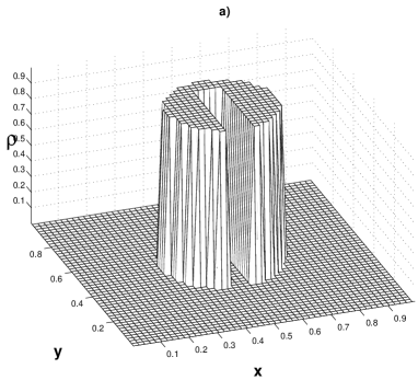
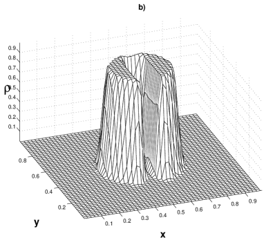
Figure 7: Two-dimensional advection. The density distributions are shown at the initial time moment (a) and after one full revolution $t=2\pi$ (b)

5.3.2 Test 7. Expansion of blast wave

The test problem of blast wave expansion in the uniform medium is very crucial for 2D numerical code due to spherical symmetry of the wave. Simulation the blast wave expansion allows us to check how precisely our 2D axisymmetrical numerical code can resolve spherically-symmetrical problems. We compute, in particular, the expansion of the supernova remnant on the adiabatic stage. This stage is described by Sedov–Taylor solution [44, 45, 46], the approximation being true while the radiation cooling is small.

We use the following initial parameters. The supernovae explosion energy is equal to $4\cdot 10^{50}~{}\mathrm{erg}$, the density of the interstellar medium $\rho_{0}\approx 2\cdot 10^{-24}~{}\mathrm{g}\cdot\mathrm{cm}^{-3}$, the spatial scale of the computational domain $R_{0}\approx 4.03\cdot 10^{19}~{}\mathrm{cm}$, the pressure in the central region differs from the pressure in the external medium at the initial time moment approximately by eight order of magnitude. The scales of the computational values are equal to: for distance — $13~{}\mathrm{pc}$, for velocity — $8.9\times 10^{8}~{}\mathrm{cm}\cdot\mathrm{s}^{-1}$, for pressure — $1.1\times 10^{-6}~{}\mathrm{erg}\cdot\mathrm{cm}^{-3}$, for time — $1510~{}\mathrm{Yrs}$. The expansion of the supernova remnant can be followed numerically over the time $t=10600~{}\mathrm{Yrs}$. The radius of the shock wave increases from $3.6~{}\mathrm{pc}$ to $12~{}\mathrm{pc}$ during this time.

Figure 8 shows the dependencies of the radius $R$, velocity $U$ and the pressure $P$ of the shock wave on the time. All curves correspond to power law: $(R,U,P)\propto t^{k}$. We obtained the following exponents: for radius of the shock wave $k_{R}=0.403$, for velocity $k_{U}=-0.589$, for pressure $k_{P}=-1.139$. The analytical values are $k_{R}=0.4$, $k_{U}=-0.6$ and $k_{P}=-1.2$. We see that the numerical values of the exponents are very close to exact Sedov–Taylor’s values. The condition of the spherical symmetry over the computations satisfies within the accuracy of 0.3%.

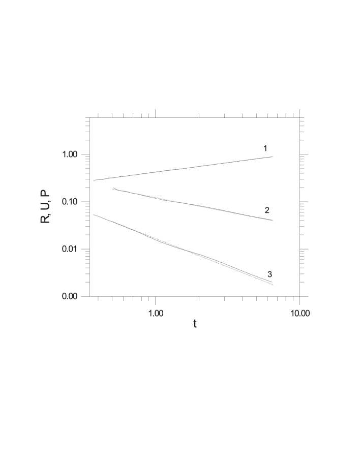
Figure 8: Expansion of blast wave. The solid lines correspond to the numerical dependencies of the radius $R$ (curve 1), velocity $U$ (curve 2) and pressure $P$ (curve 3) of shock wave behind its front of the time. The corresponding analytical dependencies are shown by dotted lines

5.3.3 Test 8. Spherically-symmetrical free-fall collapse

For simulation of free-fall (pressure-free) collapse as an initial state we take the uniform spherically-symmetrical cloud with the mass $M=1M_{\odot}$ and with the initial density $\rho_{0}=10^{-19}~{}\mathrm{g}\cdot\mathrm{cm}^{-3}$. Figure 9 shows the evolution of the numerical density (dots) of the cloud over the time in comparison with the analytical solution (solid line). We can see that the numerical points of density coincide with the high accuracy with values of the analytical solution. The cloud contracts to the point at the free-fall time $t_{ff}=\sqrt{3\pi/(32G\rho_{0})}$. The computation is carried out to time moment when the cloud size decreases to the size of one grid cell. The difference of numerical and analytical values of density is not greater than 1% at this time and the law of the spherical symmetry conservation satisfies within the accuracy of 0.4%.

Figure 9: The free-fall collapse. The numerical (dots) and the analytical (solid line) dependencies of the cloud density of the time are shown. As a unit of density it is used its initial value. As a unit of time it is used the cloud free-fall time $t_{ff}$

5.3.4 Test 9. The contraction of polytropic cloud with $\gamma=4/3$

The simulation of the selfgravitating polytropic cloud dynamics with the adiabatic index $\gamma=4/3$ allows us to check the quality and the accuracy of the code in the simulation of the selfgravitating MHD flows. The hydrostatic equilibrium of polytropic cloud with $\gamma=4/3$ is indifferent one since the total energy, its first and second variations are equal to zero (see [47]). The density distribution of this cloud can be presented by analytical form as $\rho(r)=\rho_{c}\chi^{3}(r/R)$, where $\rho_{c}$ is the central density, $R$ is the cloud radius, $\chi(x)=\theta_{3}(x/\xi_{1})$ ($\theta_{3}(\xi)$ is the Emden function of index 3 and $\xi_{1}\approx 6.9$ is its first positive zero).

To check the accuracy of the conservation of mass, momentum, and energy by our scheme we solve numerically the equations of the gravitational gasdynamics with the initial conditions corresponding to the specified hydrostatic state of the cloud. We computed several models with different numbers of cells $N$ of the spatial grid. Figure 10 shows the density profiles in the case of $N=100\times 100$. From the comparison of numerical (dots) and analytical (solid line) density profiles on this Figure we conclude that the relative error of the numerical solution compared with the analytical one at the time $t=1.5t_{ff}$ is less than 2%. The law of total mass conservation over the computations satisfies within the accuracy of 0.003% and the law of the total energy conservation satisfies within the accuracy of 2%.

Figure 10: Hydrostatic evolution of the selfgravitating polytropic cloud with $\gamma=4/3$. The analytical (solid line) and the numerical (dots) profiles of the density are shown at the time moment $t=1.5t_{ff}$

This problem was solved on the grids with the number of cells $N=20\times 20$, $80\times 80$ and $120\times 120$ as well. We can say that the relative error of the numerical solution obtained by the time $t=1.5t_{ff}$ decreases with the increasing of the cells number. In the case of $N=20\times 20$ it equals to 20% while in the case of $N=80\times 80$ — 7%, and for $N=120\times 120$ it is less than one percent. We can conclude therefore that the convergence of the numerical solution to the analytical one with the rise of the grid resolution takes place.

In another variant of this test we specified the deviation from the hydrostatic equilibrium at the initial time moment by the velocity distribution $v(r,t)=-Ur/R$. The cloud radius in this case evolves in time in accordance with the law $R(t)=R_{0}-U\cdot t$ and the evolution of the density and the velocity in the cloud can be described by the following analytical dependencies:

$$\rho(r,t)=\rho_{c}(0)\biggl{(}\frac{R_{0}}{R(t)}\chi\Bigl{(}\frac{r}{R(t)}\Bigr{)}\biggr{)}^{3}\,,\qquad\qquad u(r,t)=-U\frac{r}{R(t)}\,.$$

To the time $t_{0}=R_{0}/U$ the cloud will contract to the point.

Figure 11 shows the numerical distributions of the density (circles) and the velocity (triangles) for different times. The solid lines correspond to analytical curves. From analysis of this Figure we can conclude that the numerical solution with the high accuracy coincides with the analytical one while the grid resolution is sufficient for the adequate spatial approximation of the central region. For the variant with $N=100\times 100$ this corresponds approximately to the time moment $t=0.8t_{0}$ (see Fig. 11).

  

Figure 11: Contraction of the polytropic selfgravitating cloud with $\gamma=4/3$. The distributions of the density (a) and the velocity (b) are shown for the different moments of time. The circles and triangles correspond to the numerical solution and the solid lines correspond to the analytical one. The digits 1,2,3 correspond to the moments of time 0.0$t_{0}$, 0.69$t_{0}$ and 0.82$t_{0}$, respectively.

6 Collapse of magnetized protostellar clouds

6.1 Introduction

Protostellar clouds as the cores of interstellar molecular clouds consist of neutral (atoms, molecules and cosmic dust particles) and charged (electrons, ions and charged dust) components. The equations of similar multicomponent mixture are very complex for the numerical simulations.

The more rough ideal MHD approximation can be used as a first approach. Contracting cloud is transparent to infrared self-radiation on the early stages of collapse. Therefore the initial phases of protostellar collapse can be considered as the isothermal ones with the good approximation. This approximation works while the optical depth of the collapsing cloud core becomes comparable with the unity.

We performed the computation of the isothermal magnetized cloud collapse using the uniform grid with the cells number $N=120\times 120$ and Courant number $C=0.3$. We use the following values of parameters. The initial ratio of the thermal and kinetic rotational energies to the absolute value of the gravitational energy $\epsilon_{t}=0.386$, $\epsilon_{\omega}=0.0$, respectively. The mass of the protostellar cloud $M_{0}=1.5M_{\odot}$ and its temperature $T_{0}=10~{}\mathrm{K}$. One the basis of the relations (12–15) we can conclude that these parameters correspond to the cloud with the initial density $\rho_{0}=5.18\cdot 10^{-18}~{}\mathrm{g}\cdot\mathrm{cm}^{-3}$ and radius $R_{0}=5.17\cdot 10^{16}~{}\mathrm{cm}$. As a result of computations we calculate the flatness degree (ratio of the cloud thikness to its radius) and the central density up to the free-fall time.

6.2 Kinematics

The simplest case of the collapse corresponds to infinitesimally weak magnetic field. If the initial value $\epsilon_{m}\leq 0.5\cdot 10^{-4}$ then we can neglect the influence of the magnetic field on the collapse dynamics. The magnetic field can be considered as a passive admixture and for the given velocity field and may be determined from the equation of induction (3).

The results of computations show that in this kinematic approach the magnetic field $B\propto\rho^{k}$ with $k=2/3$ since of the cloud contraction is practically spherically-symmetrical one. Note that in the cloud envelope this law fulfills approximately and in the forming core it satisfies exactly [48]. The computations confirm the early obtained conclusion that the magnetic field in the cloud acquires with the time the quasi-radial geometry (see Fig. 12) [48]. This geometry of the field becomes distinct already to the free-fall time.

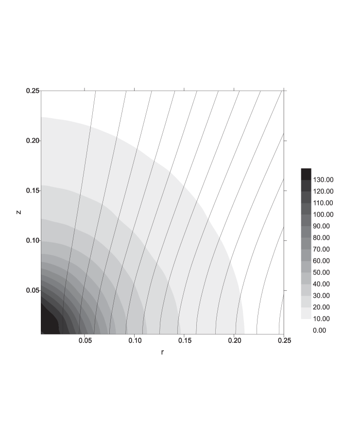
Figure 12: The density distribution and the picture of the magnetic field lines in the central region at the time moment $t=t_{ff}$ in the case of the kinematic cloud model

6.3 Dynamics

In the case of intermediate magnetic fields ($0.1\leq\epsilon_{m}\leq 0.5$) the collapse picture drastically differs from the kinematic statement. The gas particles moving across the magnetic field lines are deviated to the equatorial plane by the electromagnetic forces. As a result the flat (disk-like) structure is formed. Figure 13 shows the typical density profiles and geometry of the magnetic field lines at the moment of time equal to the magnetic free-fall time

$$t_{fm}=\sqrt{\frac{3\pi}{32G(1-\epsilon_{m})\rho_{0}}}$$

(see [48]). The magnetic field in the disk is almost quasi-uniform and the ratio $B_{r}/B_{z}$ is small.

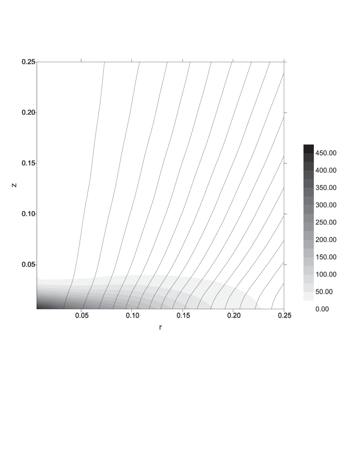
Figure 13: The density distribution and lines of equal magnetic flux in the central region of the cloud with $\epsilon_{m}=0.1$ at the time moment $t=t_{fm}$

Numerical simulations show that at the free-fall time the flatness degree of the disk is proportional to $\epsilon_{m}^{-1/2}$ and the central density is inversely proportional to $\epsilon_{m}$.

6.4 Quasi-steady-state contraction

The growth of the initial magnetic field leads to the increase of the electromagnetic forces that support the cloud from the contraction. Therefore at the large initial values $\epsilon_{m}$ the cloud relaxes to the quasi-steady-state equilibrium. Such a cloud should evolve within the diffusion time scale that is determined by the ambipolar diffusion of the magnetic field. The cloud loses the magnetic flux by the ambipolar diffusion and slowly contracts retaining the quasi-hydrostatic equilibrium. As a result this evolution the non-uniform profile of the density is formed. The lifetime of such molecular cloud cores can reach $10^{5}-10^{7}$ years.

7 Conclusion

The explicit conservative finite-difference TVD scheme of high resolution for the solution of various MHD problems is constructed. The numerical MHD code ‘Moon’ on the basis of this scheme is developed that can simulate the MHD flows in the 1D and 2D approximations. The results of extensive tests show that the code is well adapted to the simulation of many MHD problems of plasma physics and astrophysics.

To check the dissipative properties of the developed scheme the problems of 1D and 2D advection are solved. The results of these tests show that the scheme smears the initial density profile onto 3–4 cells. In the test computation of the blast wave the condition of the spherical symmetry satisfies within the accuracy of 0.3%.

To analyze the convergence of the numerical solution to the analytical one the problem of the hydrostatic equilibrium of the selfgravitating polytropic cloud with the adiabatic index $\gamma=4/3$ is computed on the grids with various number of cells. The obtained results allow us to conclude that the errors of the numerical solution decrease to the permissible values on the grids with the number of cells not less than $N=100\times 100$. In the case $N\geq 120\times 120$ the relative error of the numerical solution at the time moment $t=1.55t_{ff}$ is less that 1%. The numerical solution in this case coincides with the good accuracy with the analytical one while the grid resolution in the central region is sufficient for acceptable approximation of the grid values.

The numerical computations of the collapse of the magnetized protostellar cloud confirms the earlier obtained results in the framework of 1.5D approximation (see [48]). The magnetic field in the cloud with the initially small intensity acquires the quasi-radial geometry after some time. The intermediate magnetic field leads to flattening of the collapsing clouds on the late stages of contraction. For the strong initial magnetic field the cloud relaxes to quasi-hydrostatic equilibrium. Such a cloud must evolve within the diffusion time scale.

Note that we can not simulate numerically the advanced stages of the collapse because the described code ‘Moon’ uses the uniform grid only. But investigation of these stages is very important and interesting problem to understand the physics of the formation and further evolution of young stellar objects. We are elaborating now the adaptive mesh refinement (AMR) numerical algorithm for the simulation of advanced stages of rotating magnetized protostellar cloud collapse. The AMR-approach uses the tree-threaded collection of subgrids with the subsequently increasing grid resolution. We are constructing a new 2D MHD numerical code ‘Megalion’ that based on the described in this paper high-resolution TVD scheme for the gravitational compressible MHD flows. This code will allow us to simulate various selfgravitating MHD flows with the large gradients and fast time variations. New numerical code will take into account also the processes of ambipolar diffusion, non-stationary ionization and heating/cooling.

References

- [1] L. Spitzer, Physical processes in the interstellar medium (Wiley, New York, 1981).
- [2] A.E.Dudorov, Magnetic field of interstellar clouds, Itogy Nauki i Techniky. Astronomia 39 (1990) 71–158 (in Russian).
- [3] R.D.Richtmyer, K.W.Morton, Difference methods for initial-value problems (Wiley, New York, 1967).
- [4] G.J.Philips, J.J.Monaghan, A numerical method for three-dimensional simulations of collapsing, isothermal, magnetic gas clouds, Monthly Not. Roy. Astron. Soc. 216 (1985) 883–895.
- [5] J.P.Boris, D.L.Book, Flux-corrected transport. I. SHASTA, a fluid transport algorithm that works, J. Comput. Phys. 11 (1973) 38–69.
- [6] J.P.Boris, D.L.Book, Solution of the continuity equation by the method of flux-corrected transport, in: Methods in Computational Physics 16 (1976) 85–129.
- [7] C.R.DeVore, Flux-corrected transport techniques for multidimensional compressible magnetohydrodynamics, J. Comput. Phys. 92 (1991) 142–160.
- [8] W.Dai, P.R.Woodward, An approximate Riemann solver for ideal magnetohydrodynamics, J. Comput. Phys. 111 (1994) 354–372.
- [9] W.Dai, P.R.Woodward, A high-order Godunov-type scheme for shock interactions in ideal magnetohydrodynamics, SIAM J. Sci. Comput. 18 (1997) 957–981.
- [10] P.Colella, P.R.Woodward, The piecewise parabolic method (PPM) for gas-dynamical simulations, J. Comp. Phys. 54 (1984) 175–201.
- [11] K.G.Powell, An approximate Riemann solver for magnetohydrodynamics, ICASE Report 94-24 (1994).
- [12] K.G.Powell, P.L.Roe, T.J.Linde, T.I.Gombosi, D.L. De Zeeuw, A solution-adaptive upwind scheme for ideal magnetohydrodynamics, J. Comp. Phys. 154 (1999) 284–309.
- [13] G.S.Jiang, C.C.Wu, A high-order WENO finite difference scheme for the equations of ideal magnetohydrodynamics, J. Comp. Phys. 150 (1999) 561–594.
- [14] M.Brio, C.C.Wu, An upwind differencing scheme for the equations of ideal magnetohydrodynamics, J. Comput. Phys. 75 (1988) 400–422.
- [15] A.L.Zachary, P.Colella, A higher-order Godunov method for the equations of ideal magnetohydrodynamics, J. Comput. Phys. 99 (1992) 341–347.
- [16] A.L.Zachary, A.Malagoli, P.Colella, A high-order Godunov method of multidimensional ideal magnetohydrodynamics, SIAM J. Sci. Comput. 15 (1994) 263–284.
- [17] A.V.Koldoba, O.A.Kuznetsov, G.V.Ustyugova, Quasi-monotonic difference schemes of high-order approximation for MHD equations, preprint of Keldysh Institute of Applied Mathematics N 69 (1992, in Russian).
- [18] D.Ryu, T.M.Jones, Numerical magnetohydrodynamics in astrophysics. Algorithm and tests for one-dimensional flow, Astrophys. J. 442 (1995) 228–258.
- [19] D.Ryu, T.M.Jones, A.Frank, Numerical magnetohydrodynamics in astrophysics. Algorithm and tests for multidimensional flow, Astrophys. J. 442 (1995) 785–976.
- [20] D.S.Balsara, Linearized formulation of the Riemann problem for adiabatic and isothermal magnetohydrodynamics, Astrophys. J. Suppl. 116 (1998) 119–131.
- [21] A.E.Dudorov, A.G.Zhilkin, O.A.Kuznetsov, Quasi-monotonic difference scheme of high resolution for magnetohydrodynamics, Mat. Modelirovanie 11 N1 (1999) 101–116 (in Russian).
- [22] A.E.Dudorov, A.G.Zhilkin, O.A.Kuznetsov, The two-dimensional numerical code for simulation of axisymmetrical selfgravitating MHD flows, Mat. Modelirovanie 11 N11 (1999) 109–127 (in Russian).
- [23] A.Harten, On a class of high resolution total-variation-stable finite-difference schemes, SIAM. J. Numer. Anal. 24 (1984) 1–23.
- [24] C.V.Vyaznikov, V.F.Tishkin, A.P.Favorsky, Construction of quasi-monotonic difference schemes of high-order approximation for hyperbolic type systems of equations, Mat. Modelirovanie 1 N5 (1989) 95–120 (in Russian).
- [25] R.Courant, E.Isaacson, M.Rees, On the solution of nonlinear hyperbolic differential equations by finite differences, Commun. Pure Appl. Math. 5 (1952) 243–255.
- [26] A.A.Samarskii, Yu.P.Popov, Finite-difference methods of solution of gas dynamics (Nauka, Moscow, 1980, in Russian).
- [27] B. Van Leer, Towards the ultimate conservative difference scheme. II. Monotonicity and conservation combined in a second-order scheme, J. Comp. Phys. 14 (1974) 361–370.
- [28] B. Van Leer, Towards the ultimate conservative difference scheme. IV. A new approach to numerical convection, J. Comp. Phys. 23 (1977) 276–299.
- [29] P.L.Roe, Some contribution to the modelling of discontinuous flows, Lectures in Applied Math. 22 (1985) 163–183.
- [30] P.K.Sweby, High resolution schemes using flux limiters for hyperbolic conservation laws, SIAM J. Numer. Anal. 21 (1984) 995–1011.
- [31] S.R.Chakravarthy, S.Osher, A new class of high accuracy TVD schemes for hyperbolic conservation laws, AIAA Pap. N 85–0363 (1985).
- [32] R.Courant, K.O.Friedrichs, H.Lewy, Über die partiellen Differenzengleichungen der mathematischen Physik, Math. Ann. 100 (1928) 32–74.
- [33] P.D.Lax, Weak solutions of nonlinear hyperbolic equations and their numerical computations, Commun. Pure Appl. Math. 7 (1954) 159–193.
- [34] P.D.Lax, Hyperbolic systems of conservation laws II, Commun. Pure Appl. Math. 10 (1957) 537–566.
- [35] D.W.Peaceman, H.H.Rachford,Jr., The numerical solution of parabolic and elliptic differential equations, J. Soc. Ind. Appl. Math. (1955) 28–41.
- [36] J.Douglas,Jr., On the numerical integration of by implicit methods, J. Soc. Ind. Appl. Math. (1955) 42–65.
- [37] J.Douglas,Jr., H.H.Rachford,Jr., On the numerical solution of heat conduction problems in two and three space variables, Trans. Amer. Math. Soc. 82 (1956) 421–439.
- [38] G. Tóth, The constraint in shock-capturing magnetohydrodynamics codes, J. Comp. Phys. 161 (2000) 605–652.
- [39] C.R. Evans, J.F. Hawley, Simulation of magnetohydrodynamic flows – a constrained transport method, Astrophys. J. 332 (1988) 659–677.
- [40] J.U. Brackbill, D.C. Barnes, The effect of nonzero on the numerical solution of magnetohydrodynamic equations, J. Comp. Phys. 35 (1980) 426–430.
- [41] D.S.Balsara, Total variation diminishing scheme for adiabatic and isothermal magnetohydrodynamics, Astrophys. J. Suppl. 116 (1998) 133–153.
- [42] Landau L.D., Lifshitz E.M., Electrodynamics of continuous media (Pergamon, Oxford, 1980).
- [43] C.-D. Munz, On the numerical dissipation in high-resolution schemes for hyperbolic conservation laws, J. Comp. Phys. 77 (1988) 18–39.
- [44] L.I.Sedov, The expansion of strong blast waves, Prikl. Mat. i Mekh. 10 (1946) 241–250.
- [45] G.I.Taylor, The formation of a blast waves by a very intense explosion, Proc Roy. Soc. London A201 (1950) 159–186.
- [46] L.I.Sedov, Similarity and dimensional methods in mechanics (Academic Press, New York, 1959).
- [47] Ya.B.Zeldovich, I.D.Novikov, Theory of gravity and star evolution (Nauka, Moscow, 1971, in Russian).
- [48] A.E.Dudorov, Yu.V.Sazonov, Hydrodynamic collapse of magnetic interstellar clouds. 2. The role of magnetic field, Nauch. Inform. Astrosoveta 50 (1982) 98–112 (in Russian).