Constraints on Warm Dark Matter from Cosmological Reionization

Abstract

We study the constraints that high-redshift structure formation in the universe places on warm dark matter (WDM) dominated cosmological models. We modify the extended Press-Schechter formalism to derive the halo mass function in WDM models. We show that our predictions agree with recent numerical simulations at low redshift over the halo masses of interest. Applying our model to galaxy formation at high redshift, we find that the loss of power on small scales, together with the delayed collapse of low-mass objects, results in strong limits on the root-mean-square velocity dispersion $v_{\rm rms,0}$ of the WDM particles at redshift zero. For fermions decoupling while relativistic, these limits are equivalent to constraints on the mass $m_{X}$ of the particles. The presence of a $\approx 4\times 10^{9}~{}{\rm M_{\odot}}$ supermassive black hole at redshift 5.8, believed to power the quasar SDSS 1044-1215, implies $m_{X}\gtrsim 0.5$ keV (or $v_{\rm rms,0}\lesssim 0.10$ km/s), assuming that the quasar is unlensed and radiating at or below the Eddington limit. Reionization by redshift 5.8 also implies a limit on $m_{X}$. If high-redshift galaxies produce ionizing photons with an efficiency similar to their redshift-three counterparts, we find $m_{X}\gtrsim 1.2~{}$keV (or $v_{\rm rms,0}\lesssim 0.03$ km/s). However, given the uncertainties in current measurements from the proximity effect of the ionizing background at redshift three, values of $m_{X}$ as low as $0.75~{}$keV (or $v_{\rm rms,0}=0.06$ km/s) are not ruled out. The limit weakens further to $m_{X}\gtrsim 0.4~{}$keV (or $v_{\rm rms,0}\lesssim 0.14$ km/s), if, instead, the ionizing-photon production efficiency is ten times greater at high redshift, but this limit will tighten considerably if reionization is shown in the future to have occurred at higher redshifts. WDM models with $m_{X}\lesssim 1~{}$keV (or $v_{\rm rms,0}\gtrsim 0.04$ km/s) produce a low-luminosity cutoff in the high-redshift galaxy luminosity function which is directly detectable with the Next Generation Space Telescope,  and which serves as a direct constraint on $m_{X}$.

1 Introduction

The currently favored model of hierarchical galaxy formation in a universe dominated by cold dark matter (CDM) has been very successful in matching observations of the density distribution on large scales. These successes include the properties of galaxy clusters, galaxy clustering on large scales, the statistics of the Lyman-$\alpha$ forest, and the temperature anisotropy of the cosmic microwave background. However, recently some small-scale shortcomings of this model have appeared (see Sellwood & Kosowsky, 2000, for a recent review). CDM models predict dense, cuspy dark matter halo profiles (Navarro, Frenk, & White, 1997; Moore et al., 1998; Subramanian, Cen, & Ostriker, 2000; Klypin et al., 2000) which are not apparent in the mass distribution derived from measurements of the rotation curves of dwarf galaxies (e.g., de Blok & McGaugh, 1997; Salucci & Burkert, 2000), although observational and modeling uncertainties may preclude a firm conclusion at present (van den Bosch et al., 2000; Swaters, Madore, & Trewhella, 2000). Dense dark matter halos may contradict observational indications of fast-rotating bars in galaxies (Debattista & Sellwood, 1998; Weiner, Sellwood, & Williams, 2000, but see Tremaine & Ostriker 1999 for a counterargument). Halos with lower central densities than in CDM also appear necessary to explain the observed normalization of the Tully-Fisher relation (Navarro & Steinmetz, 2000; Mo & Mao, 2000, but see the reassessment by Eke, Navarro & Steinmetz 2001). In addition, the abundance of satellites and dwarf galaxies in the Local Group is apparently lower by an order of magnitude than the abundance of corresponding halos in numerical simulations of CDM (Klypin et al., 1999; Moore et al., 1999). Finally, the halo profiles expected in CDM may conflict with observed lensing statistics (Li & Ostriker, 2001; Keeton & Madau, 2001).

Although the significance of these discrepancies is still disputed, and astrophysical solutions involving feedback may still be possible, the accumulating tension with observations has focused attention on solutions involving the particle properties of dark matter. Self-interacting dark matter particles can heat the low-entropy particles which would otherwise create a dense core, and result in flatter halo profiles (Spergel & Steinhardt, 2000; Burkert, 2000; Firmani et al., 2000; Davé et al., 2000, but see Miralda-Escudé 2000; Kochanek & White 2000; Yoshida et al. 2000 and Gnedin & Ostriker 2000 for possible conflicts of the simplest models with observations). Self-interacting dark matter particles in the initial state of a cold Bose-Einstein condensate, with a repulsive interaction added to gravity, can also suppress halo cores (Goodman, 2000; Peebles, 2000). Alternatively, even with no interaction other than gravity, the quantum-mechanical wave properties of ultra-light ($\sim 10^{-22}$ eV) dark matter particles stabilize gravitational collapse, providing halo cores and sharply suppressing the small-scale linear power spectrum (“Fuzzy CDM”; Hu, Barkana, & Gruzinov, 2000). Finally, a resurrection of warm dark matter (WDM) models (Pagels & Primack, 1982; Blumenthal, Pagels, & Primack, 1982; Pierpaoli et al., 1998) has recently been proposed (Colín, Avila-Reese, & Valenzuela, 2000; Sommer-Larsen & Dolgov, 2000; Bode, Ostriker, & Turok, 2000). By design, a common feature of models that attempt to solve the apparent “small-scale” problems of CDM is the reduction of power on small scales. In the CDM paradigm, structure formation proceeds “bottom-up”, i.e., the smallest objects collapse first, and they subsequently merge together to form larger objects. It then follows that the loss of small-scale power modifies structure formation most severely at the highest redshifts; in particular, the number of self-gravitating objects at high redshift is reduced.

A strong reduction in the abundance of high-redshift objects would, however, be in conflict with the observed reionization of the universe. The lack of a Gunn-Peterson trough in the spectra of high-redshift quasars implies that the hydrogen in the intergalactic medium (IGM) was highly ionized throughout the universe. In particular, the spectrum of the bright quasar SDSS 1044-1215 at redshift $z=5.8$ (Fan et al., 2000) shows transmitted flux short-ward of the Ly$\alpha$ wavelength, implying that reionization was complete by $z=5.8$ Note that recent observations of small-scale anisotropies of the cosmic microwave background radiation (de Bernardis et al., 2000; Hanany et al., 2000) can be used to also place an upper limit of $z\lesssim 30$ on the reionization redshift (Tegmark & Zaldarriaga, 2000). The most natural explanation for reionization is photo-ionizing radiation produced by an early generation of stars and quasars; recent calculations of structure formation in $\Lambda$CDM find that reionization should naturally occur at $z\sim 7$–12 (Haiman & Loeb, 1997, 1998; Gnedin & Ostriker, 1997; Chiu & Ostriker, 2000; Gnedin, 2000, and for a recent review of reionization, see Barkana & Loeb 2001). In these models, the sources of reionization reside in halos that have masses in the range corresponding to dwarf galaxies — the mass scale on which power needs to be reduced relative to CDM models.

In this paper, we examine the constraints that arise from the reionization of the universe. We focus on WDM models, although similar constraints would apply to other modifications of the CDM paradigm that reduce the small-scale power. Our goal is to quantify the allowed mass range of WDM particles, given the evidence that the universe was reionized by a redshift $z>5.8$. The rest of this paper is organized as follows. In § 2 we review the basic properties of WDM models. In § 3 we describe our methods of modeling the formation and abundance of WDM halos, as well as reionization. In § 4 we present our main results, namely, the limits on the WDM particle mass. Finally, in § 5, we summarize our conclusions and the implications of this work. Unless stated otherwise, in the case of CDM, we adopt the $\Lambda$CDM parameters $\Omega_{0}=0.3$, $\Omega_{\Lambda}=0.7$, and $\Omega_{\rm b}=0.045$ for the energy density ratios relative to the critical density of matter, vacuum, and baryons, respectively. We also assume a Hubble constant $H_{0}=100\,h~{}{\rm km~{}s^{-1}~{}Mpc^{-1}}$ with $h=0.7$, and a primordial scale invariant ($n=1$) power spectrum with $\sigma_{8}=0.9$, where $\sigma_{8}$ is the root-mean-square amplitude of mass fluctuations in spheres of radius $8\ h^{-1}$ Mpc. These parameter values are based primarily on observations of cosmological expansion and large-scale structure (summarized, e.g., in Bahcall et al., 1999) and degree-scale temperature anisotropy measurements in the cosmic microwave background (de Bernardis et al., 2000; Hanany et al., 2000). If CDM is replaced by WDM with similar cosmological parameters, the resulting model (in which the contribution of WDM to $\Omega$ equals $\Omega_{0}-\Omega_{\rm b}$) is termed $\Lambda$WDM.

2 Warm Dark Matter Models

In this paper we focus on WDM models, which attempt to improve over CDM by reducing small-scale power. The WDM is assumed to be composed of particles of about a keV mass (rather than a GeV as often assumed for CDM). In this case, the particles are not completely cold: thermal velocities on the order of 1 km/s at the time of reionization produce free streaming whereby particles stream out of overdense regions. This smoothes out small regions, leading to a small-scale cutoff in the linear power spectrum, and it also acts similarly to pressure and substantially delays the formation of small halos.

We assume that the WDM is composed of particles of mass $m_{X}$ which decouple in the early universe while relativistic and in thermal equilibrium (see, e.g., Kolb & Turner, 1990). The initial Fermi-Dirac distribution function for the momentum $p$ is given by $\left\{\exp\left[(pc)/(k_{B}T_{X})\right]+1\right\}^{-1}\,$, in terms of the temperature $T_{X}$. Since both relativistic and non-relativistic momenta redshift as $1/a$, where $a$ is the scale factor, the distribution function remains self-similar as the universe expands, with the effective temperature $T_{X}$ (which equals the actual temperature as long as the WDM is relativistic) also redshifting as $1/a$. At WDM decoupling, $T_{X}$ equals the photon temperature $T$, but later annihilating species transfer their entropy to the photons (and to other particles in thermal equilibrium with the photons) but not to the WDM. As a result, today $T_{X}/T=\left[(43/11)/g_{\rm dec}\right]^{1/3}$, where $g_{\rm dec}$ is the effective number of relativistic species present at WDM decoupling, and 43/11 is the number today, assuming three massless neutrino species. The present number density $n_{X}$ of WDM relative to that of photons equals $(T_{X}/T)^{3}g_{X}/2$, where $g_{X}$ is the effective number of degrees of freedom of WDM. Bosonic degrees of freedom contribute unity, and fermionic ones contribute 7/8 to $g_{\rm dec}$ (which measures entropy density) and 3/4 to $g_{X}$ (which measures number density). Thus, the usual assumption of a fermionic spin-$1/2$ particle implies $g_{X}=1.5$.

To produce a given contribution $\Omega_{X}$ to the cosmological critical density, the required mass is determined by $m_{X}n_{X}\propto\Omega_{X}h^{2}$. The above distribution function at low redshift has the form $\left\{\exp\left[v/v_{0}\right]+1\right\}^{-1}\,,$ where we used the fact that $p=m_{X}v$ (with $v$ the physical, peculiar velocity) after the WDM particles become non-relativistic. The root-mean-square velocity is $v_{\rm rms}=3.597\,v_{0}$, where $m_{X}v_{0}=k_{B}T_{X}/c\propto(n_{X}/g_{X})^{1/3}$. These relations can be combined to yield a formula relating $v_{\rm rms}$ to $m_{X}$,

$$v_{\rm rms}(z)=0.0437\left(1+z\right)\left(\frac{\Omega_{X}h^{2}}{0.15}\right)^{1/3}\left(\frac{g_{X}}{1.5}\right)^{-1/3}\left(\frac{m_{X}}{\rm 1~{}keV}\right)^{-4/3}~{}{\rm km~{}s^{-1}}\ .$$ (1)

Although not directly relevant to the astrophysics of WDM, a fundamental aspect of the particle physics is the required value of

$$g_{\rm dec}=766\left(\frac{\Omega_{X}h^{2}}{0.15}\right)^{-1}\left(\frac{g_{X}}{1.5}\right)\left(\frac{m_{X}}{\rm 1~{}keV}\right)\ .$$ (2)

Since this is larger by a factor of $\sim 7$ than the number of degrees of freedom in the standard model, WDM requires physics beyond the standard model (see, e.g., the discussion in Bode et al., 2000). Other alternatives for the origin of the velocities are possible (e.g., non-thermal production of weakly interacting massive particles, see Lin et al. 2001); the critical element is the value of $v_{\rm rms}$, which can always be parameterized as $v_{\rm rms}=(1+z)\,v_{\rm rms,0}$. As noted above, for the fiducial model considered here, $v_{\rm rms,0}\approx 0.05~{}{\rm km~{}s^{-1}}$.

The growth of linear perturbations in WDM models can be calculated by solving the Einstein-Boltzmann equations. The resulting linear power spectrum can be written as the CDM power spectrum (which we compute using Eisenstein & Hu, 1999) times the square of a transfer function. For $z=0$, the transfer function is (Bode et al., 2000)

$$T_{X}(k)=\left(1+(\epsilon kR_{c}^{0})^{2\nu}\right)^{-\eta/\nu}\ ,$$ (3)

with parameters $\epsilon=0.361$, $\eta=5$ and $\nu=1.2$. The comoving cutoff scale $R_{c}^{0}$, defined so that at $k=1/R_{c}^{0}$ the power spectrum is reduced in half compared to CDM, is given by

$$R_{c}^{0} = 0.201\left(\frac{\Omega_{X}h^{2}}{0.15}\right)^{0.15}\left(\frac{g_{X}}{1.5}\right)^{-0.29}\left(\frac{m_{X}}{\rm 1~{}keV}\right)^{-1.15}~{}{\rm Mpc}\$$ (4)

$$= 0.226\left(\frac{\Omega_{X}h^{2}}{0.15}\right)^{-0.14}\left(\frac{v_{\rm rms,0}}{\rm 0.05~{}km/s}\right)^{0.86}~{}{\rm Mpc}\ .$$

In our calculations below we also require the WDM power spectrum at matter-radiation equality, $z=z_{\rm eq}$. Based on results from a Boltzmann code (C.-P. Ma, personal communication), we find for $\Omega_{X}=0.3$ and $h=0.7$ an accurate fitting formula for $T_{X}(k)$ of the same form as above, but with parameters $\epsilon=0.359$, $\eta=3.81$ and $\nu=1.1$. In this case, the cutoff scale is $R_{c}^{\rm eq}=0.932R_{c}^{0}$. As expected, at equality the cutoff in the power spectrum is less sharp than at $z=0$, and so $\eta$ is smaller. At either redshift, we can define a characteristic mass $M_{c}$ from the characteristic scale $R_{c}$ using the mean density of the universe, and thus

$$M_{c}=1.74\times 10^{8}\left(\frac{\Omega_{0}h^{2}}{0.15}\right)\left(\frac{R_{c}}{\rm 0.1~{}Mpc}\right)^{3}~{}M_{\sun}\ .$$ (5)

As we discuss in detail below, the effect of free streaming is to suppress the formation of small WDM halos. This is especially true at high redshift, when only the rare, most overdense peaks collapse, and even a small delay in the collapse of each halo can greatly reduce the abundance of halos. Since these small halos merge to create the dense cores of later halos in CDM models, low-redshift halos in WDM are less centrally-concentrated and have shallower density profiles. Numerical simulations confirm that WDM models provide a closer match to observations of dwarf galaxies, in terms of their abundance and structure (Colín et al., 2000; Bode et al., 2000; Eke, Navarro & Steinmetz, 2001), the sizes of their gaseous disks (Sommer-Larsen & Dolgov, 2000), and their spatial distribution and formation epoch (Bode et al., 2000). The observed scaling of central phase-space density with mass, in objects ranging from dwarf galaxies to galaxy clusters, is inconsistent with the simple idea of an initial phase-space density which remains conserved; however, only the averaged, coarse-grained phase-space density is accessible to observations, which therefore imply that the coarse-grained density of most objects must have significantly decreased during the hierarchical formation process (Dalcanton & Hogan, 2000; Sellwood, 2000). Still, since the phase-space density can only decrease (in the absence of dissipation), the high phase-space densities of dwarf spheroidal galaxies imply a minimum mass of $m_{X}\sim 0.7$ keV for thermal WDM (Dalcanton & Hogan, 2000). The precise limit depends on the assumption that the DM core radius in the dwarf spheroidals is roughly twice the observed core radius in the stellar distribution. If the ratio is four rather than two then the mass limit weakens to $m_{X}\sim 0.4$ keV. An independent limit on $m_{X}$ has been derived based on a comparison of $z\sim 3$ observations and numerical simulations; requiring the WDM model to match the observed opacity distribution of the Lyman-$\alpha$ forest results in a lower limit of $m_{X}\sim 0.75$ keV (Narayanan et al., 2000).

In this paper we derive a new, independent constraint on WDM models. If the problem of dwarf galaxy density profiles is solved by invoking WDM, the resulting strong suppression of the abundance of dwarf galaxies at high redshift may be inconsistent with the observed fact of the reionization of the universe, since precisely these galaxies must produce the reionization.

3 Modeling Methods

3.1 Halo Formation in WDM

To understand the properties of halos in WDM, the non-linear problem of gravitational collapse must be considered. The dynamical collapse of a dark matter halo can be solved analytically only in cases of particular symmetry. In particular, spherical collapse has proven very useful in understanding the properties and distribution of halos in CDM, particularly since the results enter into the Press-Schechter model for the halo abundance. Thus, as a first step in building a semi-analytic model for WDM, we consider in this section the formation of WDM halos under spherical symmetry.

In CDM, spherical collapse is simple enough that it can be solved analytically. For an initial top-hat perturbation, different mass-shells do not cross until the final collapse and virialization. The motion of each shell is simply determined by the enclosed mass, which is fixed, and thus the turnaround and collapse times can be calculated, with the final radius derived from the radius at turnaround together with the virialization condition. The corresponding problem in WDM is, however, much more challenging, even once a numerical approach is adopted. The particles making up each mass shell start out with random velocities as given by the Fermi-Dirac distribution function (§2). Even in the initial stages, particles from different mass shells mix, and the velocity distribution function at each radius changes shape. For an accurate numerical solution, the full velocity distribution function at each radius must be well resolved, as opposed to the single shell velocity which suffices in the CDM case. We defer to later work the full implementation of WDM in spherical collapse simulations, and instead we focus on a simpler model which closely approximates the physics of WDM.

This alternative physical system, which we use as a model for WDM, is an adiabatic gas, with an initial temperature which corresponds to the initial velocity dispersion of the WDM. We emphasize for clarity that this gas does not correspond to baryons but is instead a model for WDM. To set up the analogy in the initial nearly-homogeneous universe, we match the root-mean-square velocities of the (non-relativistic) WDM and the analogous gas. This requires a gas temperature $T$ where

$$v_{\rm rms}^{2}=3k_{B}T/\mu\ ,$$ (6)

in terms of the mean molecular mass $\mu$ chosen for the gas. The conservation of phase-space density for WDM yields $v_{\rm rms}\propto\rho^{1/3}$, equivalent to an adiabatic gas with pressure $p\propto\rho^{\gamma}$ where the index $\gamma=5/3$. It is easy to show that, in the simple case of a homogeneous expanding universe, the WDM and gas models are mathematically identical. The decline of $v_{\rm rms}$ as $1/a$ for WDM corresponds to the adiabatic cooling $T\propto 1/a^{2}$ for the gas. During the collapse, the conservation of phase-space density yields an effective equation of state, although the analogy to gas is not exact because it does not precisely capture the effect of shell mixing and it neglects anisotropic stress. Furthermore, there is a fundamental difference in the behavior of small-scale modes in the two cases; these modes decay in the case of free streaming, but they remain constant in amplitude and oscillate as sound waves in the case of gas pressure. Nonetheless, for our purposes the key is in the similarity of free streaming and gas pressure when they compete with gravity; both effects allow the growth of fluctuations above a characteristic mass scale and prevent it below that scale. Numerically, the required initial gas temperature at $z=z_{i}$ is

$$T=9.1\times 10^{5}\left(\frac{\mu}{m_{p}}\right)\left(\frac{v_{\rm rms,0}}{\rm 0.05~{}km/s}\right)^{2}\left(\frac{1+z_{i}}{3000}\right)^{2}\,K\ ,$$ (7)

where $m_{p}$ is the proton mass.

We simulate spherical WDM/gas collapse using an improved version of the code presented in Haiman, Thoul & Loeb (1996) and originally developed by Thoul & Weinberg (1995). This is a one-dimensional, spherically symmetric Lagrangian hydrodynamics code. For initial conditions at time $t_{i}$ we assume spatial fluctuations in the WDM density in the form of a single spherical Fourier mode,

$$\frac{\rho(r,t_{i})-\bar{\rho}(t_{i})}{\bar{\rho}(t_{i})}=\delta(t_{i})~{}\frac{\sin(kr)}{kr}\ ,$$ (8)

where $\bar{\rho}(t_{i})$ is the background density of WDM at $t_{i}$, $\delta(t_{i})$ is the initial overdensity amplitude, $r$ is the comoving radial coordinate, and $k$ is the comoving perturbation wavenumber. We define the halo mass as the initial mass inside the radius given by $kr=\pi$. For the initial redshift $z_{i}$ we choose matter-radiation equality,

$$1+z_{\rm eq}=3600\left(\frac{\Omega h^{2}}{0.15}\right)\ .$$ (9)

Since for reionization we must be able to predict the halo mass function as early as $z=20$–30, in order to begin in the linear regime we must choose $z_{i}\gg 100$. Furthermore, as shown below, most of the effect of WDM that causes the delay in halo collapse occurs at very high redshift, so in order to include the entire effect it is necessary to begin at $z_{\rm eq}$ at which time density perturbations begin to grow significantly.

Figure 1 shows an example of shell trajectories for gas corresponding to $\Lambda$WDM with $m_{X}=1$ keV ($v_{\rm rms,0}=0.041~{}$km/s; solid curves) and for gas corresponding to $\Lambda$CDM (dashed curves). The trajectories are shown for four different mass shells, where the second-highest shell corresponds to the halo mass of $1.6\times 10^{8}M_{\odot}$. Each shell reaches a radius of maximum expansion and then contracts until it is stopped by the outward-moving virialization shock. In the case of WDM particles a similar trajectory shape would arise, if we consider the radius of a shell enclosing a fixed mass, with shocking replaced by violent relaxation occurring due to rapid shell mixing. By comparing the different curves in the figure, we calculate the delay relative to $\Lambda$CDM in the virialization redshift, caused by the WDM velocities. For the different mass shells shown in the figure, the delay factor in the value of $(1+z)$ at virialization ranges from 1.99–2.09, and the increase in the radius at virialization ranges from 2.12–2.19. Each of these ranges is narrow, and thus the results are insensitive to the halo density profile. Also, the two factors (for $(1+z)$ and for the radius) are nearly equal, which implies that the virialization radius in WDM is smaller than it would be in CDM, for the same  virialization redshift, by only $\sim 5\%$ for this halo mass. We find in general that although the halo virialization is delayed in WDM, and the final halo radius is larger than in CDM, the homogeneous background universe also expands significantly during this extra period; the final halo overdensity relative to the cosmological mean at the virialization time is almost unchanged, and we neglect the small change that may occur.

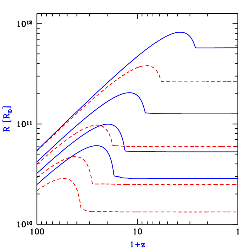
Figure 1: Example of shell trajectories for gas with initial temperature corresponding to $\Lambda$WDM with $m_{X}=1$ keV ($v_{\rm rms,0}=0.041~{}$km/s; solid curves) and for gas with initial $T=0$ K (corresponding to $\Lambda$CDM; dashed curves). In each case, four trajectories are shown, in order of increasing enclosed mass (from bottom to top). The curves correspond to enclosed masses of $1/4$, $1/2$, 1 and 2, respectively, in units of $1.6\times 10^{8}M_{\odot}$ which is the mass of the halo in this case.

In this gas model of WDM, the delayed collapse of halos is due to pressure, and the characteristic halo mass below which a significant effect occurs is the Jeans mass. In general, the Jeans mass $M_{J}$ is the halo mass for which pressure just balances gravity initially (in the linear regime). For a temperature $T$ and density $\rho$, $M_{J}\propto T^{3/2}/\rho^{1/2}$. For WDM this yields,

$$M_{J} = 3.06\times 10^{8}\left(\frac{g_{X}}{1.5}\right)^{-1}\left(\frac{\Omega_{X}h^{2}}{0.15}\right)^{1/2}\left(\frac{m_{X}}{\rm 1~{}keV}\right)^{-4}\left(\frac{1+z_{i}}{3000}\right)^{3/2}~{}M_{\sun}\$$ (10)

$$= 4.58\times 10^{8}\left(\frac{\Omega_{X}h^{2}}{0.15}\right)^{-1/2}\left(\frac{v_{\rm rms,0}}{\rm 0.05~{}km/s}\right)^{3}\left(\frac{1+z_{i}}{3000}\right)^{3/2}~{}M_{\sun}\ .$$

The collapse simulations confirm these scalings. Indeed, for a given collapse delay factor, the affected halo mass varies with $m_{X}$ and with $z_{i}$ just as $M_{J}$ does. In particular, it is necessary to start the simulations at $z_{\rm eq}$, since the effective pressure of WDM affects the highest halo masses at the highest redshifts. If we were to begin the simulations at a lower $z_{i}$, with identical initial conditions in WDM and CDM, the comparison would not include the full effect of WDM, since it would not include the effect at $z>z_{i}$ of WDM pressure on the collapse.

3.2 Halo Abundances in WDM

In addition to characterizing the properties of individual halos, a critical prediction of any theory of structure formation is their mass function, i.e. the abundance of halos as a function of mass, at each redshift. This prediction is an important step towards inferring the abundance of galaxies. While the number density of halos can be measured for particular cosmologies in numerical simulations, an analytic model helps us gain physical understanding and can be used to explore the dependence of abundances on redshift and on all model parameters.

A simple analytic model which successfully matches many numerical simulations of CDM was developed by Press & Schechter (1974). The model is based on the ideas of a Gaussian random field of initial density perturbations, linear gravitational growth, and spherical collapse. The abundance of halos at redshift $z$ is determined using $\delta_{M}$, the density field smoothed on a mass scale $M$. The variance $\langle\delta_{M}\rangle^{2}$ is denoted $\sigma^{2}(M)$, where the conventional filter is a top-hat of comoving radius $R$, with $M=4\pi\rho_{m}R^{3}/3$, in terms of the current mean density of matter $\rho_{m}$. Although the Press-Schechter model is based on the initial conditions, it is usually expressed in terms of redshift-zero quantities. Thus, it uses the linearly-extrapolated density field, i.e., the initial density field at high redshift extrapolated to the present by simple multiplication by the relative growth factor.

Since $\delta_{M}$ is distributed as a Gaussian variable with zero mean and standard deviation $\sigma(M)$ [which depends only on the present linearly-extrapolated power spectrum], the probability that $\delta_{M}$ is greater than some threshold $\delta$ equals

$$\int_{\delta}^{\infty}d\,\delta_{M}\frac{1}{\sqrt{2\pi}\,\sigma(M)}\exp\left[-\frac{\delta_{M}^{2}}{2\,\sigma^{2}(M)}\right]={1\over 2}\,{\rm erfc}\left[\frac{\delta}{\sqrt{2}\,\sigma(M)}\right]\ .$$ (11)

The fundamental ansatz of Press & Schechter was to identify this probability with the fraction of DM particles which are part of collapsed halos of mass greater than $M$ at redshift $z$, with two additional ingredients: First, the value used for $\delta$ is $\delta_{\rm crit}(z)$, which is the critical density of collapse found for a spherical top-hat (extrapolated to the present since $\sigma(M)$ is also calculated using the linear power spectrum extrapolated to the present); and second, the fraction of DM in halos above $M$ is multiplied by an additional factor of 2 in order to ensure that every particle ends up as part of some halo with $M>0$. Thus, the final formula for the mass fraction in halos above $M$ at redshift $z$ is

$$F(>M|z)={\rm erfc}\left(\frac{\nu}{\sqrt{2}}\right)\ ,$$ (12)

where $\nu=\delta_{\rm crit}(z)/\sigma(M)$ is the number of standard deviations which the critical collapse overdensity represents on mass scale $M$. Expressing this as $F(>\nu|z)$ yields the mass function

$$\nu f(\nu)\equiv-\nu\frac{dF(>\nu|z)}{d\nu}=\sqrt{\frac{2}{\pi}}\,\nu\,\exp\left[-\frac{\nu^{2}}{2}\right]\ .$$ (13)

The comoving number density $dn$ of halos of mass between $M$ and $M+dM$ is given by

$$\frac{dn}{dM}=\frac{\rho_{m}}{M}\,\frac{-d(\ln\sigma)}{dM}\nu f(\nu)\ .$$ (14)

As noted above, the ad-hoc correction by a factor of two is necessary, since otherwise only positive fluctuations of $\delta_{M}$ would be included. Bond et al. (1991) found an alternate derivation of this correction factor, using a different ansatz. In their derivation, the factor of two has a more satisfactory origin, namely the so-called “cloud-in-cloud” problem: For a given mass $M$, even if $\delta_{M}$ is smaller than $\delta_{\rm crit}(z)$, it is possible that the corresponding region lies inside a region of some larger mass $M_{L}>M$, with $\delta_{M_{L}}>\delta_{\rm crit}(z)$. In this case the original region should be counted as belonging to a halo of mass $M_{L}$. Thus, the fraction of particles which are part of collapsed halos of mass greater than $M$ is larger than the expression given in equation (11).

Bond et al. (1991) considered how to determine the mass of the halo which contains a given point $\bf{O}$. They examined the value of $\delta_{M}$ as a function of $M$ about the point $\bf{O}$, starting with $\delta_{M}=0$ as $M\rightarrow\infty$, with $\delta_{M}$ increasing as smaller regions are considered. They proposed to find the largest value of $M$ for which $\delta_{M}$ is sufficiently large [i.e., above $\delta_{\rm crit}(z)$] to correspond to a collapsed halo. Since this mass corresponds to the largest collapsed halo around $\bf{O}$, associating this halo with the point $\bf{O}$ naturally solves the cloud-in-cloud problem. To further simplify the derivation, in the smoothing kernel used to define $\delta_{M}$ Bond et al. (1991) used a $k$-space top-hat filter rather than a top-hat in real space. This way, as $M$ is lowered, new $k$ values enter which, for a Gaussian random field, are uncorrelated with those previously included. This results in a random walk whose statistics are determined by the variance $S=\sigma^{2}(M)$. Starting at $\delta_{M}=0$ when $S=0$, the first crossing of $\delta_{M}$ above the barrier $B=\delta_{\rm crit}(z)$ yields the mass of the halo containing $\bf{O}$. Performing many such random walks results in the halo abundance, where the mass fraction in halos with mass between $M_{1}$ and $M_{2}$ equals the fraction of random walks which first cross above the barrier $B$ between $S(M_{1})$ and $S(M_{2})$. Since the barrier is constant (i.e., independent of $M$) in CDM, Bond et al. (1991) could derive the halo abundance analytically, and showed that this solution to the cloud-in-cloud problem results precisely in a factor-of-two correction to equation (11). Although the Bond et al. (1991) derivation uses $\sigma(M)$ as defined by a $k$-space top-hat filter, the final formula is usually applied using a real-space top-hat. We follow this convention throughout this paper.

The cloud-in-cloud correction is more complicated in the case of WDM. As shown in the previous subsection, halo collapse is delayed when the velocity dispersion of WDM is included. Thus, the collapse threshold $\delta_{\rm crit}$ becomes a function of $M$ as well as $z$ (Note that the linear extrapolations used to define $\delta_{\rm crit}$ and $\sigma(M)$ use the growth factor as calculated in $\Lambda$CDM). A grid of collapse simulations in ($z,M$) as described above, can be used to derive the full function $\delta_{\rm crit}(z,M)$ for different values of $m_{X}$. In addition, the cut-off in the power spectrum due to free streaming by the WDM particles lowers the value of $\sigma(M)$ compared to that in CDM. Note that since we determine $\delta_{\rm crit}$ based on simulations that are run from matter-radiation equality, for consistency we calculate $\sigma(M)$ based on the WDM power spectrum at equality. In WDM, $\sigma(M)$ approaches a constant value as $M\rightarrow 0$, unlike CDM where it continues to rise logarithmically. On the other hand, the barrier height $\delta_{\rm crit}$ diverges in WDM as $M\rightarrow 0$, while it is constant in CDM. Thus, in CDM the expression on the right-hand side of equation (11) increases monotonically as the mass is lowered, while in WDM this same expression (with $\delta=\delta_{\rm crit}$) reaches a maximum and then declines toward zero as $M\rightarrow 0$. Thus, a naive application to WDM of equation (11) fails, and the cloud-in-cloud correction is crucial in this case. We derive the halo mass fraction $F(>M|z)$ in WDM by numerically generating random walks and counting the distribution of their first crossings of the barrier $B=\delta_{\rm crit}(z,M)$.

An additional ingredient is necessary for calculating an accurate mass function. Even in $\Lambda$CDM, the Press-Schechter halo mass function disagrees somewhat with that measured in numerical simulations. Specifically, the simulations find larger numbers of rare, massive halos but smaller numbers of the more abundant low-mass halos. Sheth & Tormen (1998) fitted the mass function seen in simulations with a function of the form:

$$\nu f(\nu)=\sqrt{2}{\pi}A\left(1+\frac{1}{\hat{\nu}^{2q}}\right)\hat{\nu}\exp\left(-\frac{\hat{\nu}^{2}}{2}\right)\ ,$$ (15)

where $\hat{\nu}=\sqrt{a}\nu$, and the fitted parameters are $a=0.707$, $q=0.3$, and $A=0.322$. Sheth, Mo, & Tormen (2000) showed numerically that this correction to the Press-Schechter mass function is equivalent to changing the barrier shape from the case of the constant barrier $B_{0}=\delta_{\rm crit}(z)$. Namely, the “naive” barrier $B_{0}$ must be mapped to the actual barrier by

$$B=\sqrt{a}\,B_{0}\left[1+b\left(\frac{\sigma^{2}(M)}{aB_{0}^{2}}\right)^{c}\,\right]\ ,$$ (16)

where $a$ is the same as before and also $b=0.5$ and $c=0.6$. Sheth et al. (2000) also show that if the effect of shear and ellipticity on halo collapse is considered, the resulting barrier $B$ is modified from $B_{0}$ (which is based on spherical collapse) in a way that is similar to the above fit, except with $a=1$. In particular, ellipticity does not explain the under-prediction of the number of massive halos. Thus, ellipticity explains the need for a more complicated barrier shape than is suggested by spherical halo collapse, but the precise shape needed to fit the simulations may indicate the presence of additional effects.

Regardless of the precise physical explanation, the mapping given by equation (16) can be applied to produce mass functions which agree with numerical simulations of $\Lambda$CDM. Assuming that the same mapping applies to WDM as well, we apply this mapping to the “naive” WDM barrier $B_{0}=\delta_{\rm crit}(z,M)$ to derive the final barrier shape. More precisely, we use the mass function with slightly different parameters as specified by Jenkins et al. (2000), who fitted a number of simulations with a larger range of halo mass and redshift. We note that Jenkins et al. (2000) adopted a somewhat unconventional definition of halo mass when they derived their mass function (enclosing 180 times the background density, as in the Einstein-deSitter model, rather than the value suggested by spherical collapse in $\Lambda$CDM). In the present application at high redshift, where $\Omega(z)\approx 1$, this has little effect on the mass function (see also White, 2000, for a general discussion of the effect of the halo mass definition on the mass function). The fitting parameters found by Jenkins et al. (2000) are $a=0.73$, $q=0.175$, and $A=0.353$ in equation (15). We find numerically that this mass function is approximately generated if $b=0.34$ and $c=0.81$ are chosen in equation (16). Figure 2 shows the resulting value of $\delta_{\rm crit}$ (top panel) as a function of halo mass $M$, at $z=6$. Also shown (bottom panel) is the mass fluctuation $\sigma(M)$. The $\Lambda$WDM models correspond to $m_{X}=1.5$ keV ($v_{\rm rms,0}=0.024~{}$km/s; $R_{c}=0.12\,$Mpc; $M_{c}=3.1\times 10^{8}M_{\odot}$) and $m_{X}=0.75$ keV ($v_{\rm rms,0}=0.060~{}$km/s; $R_{c}=0.27\,$Mpc; $M_{c}=3.4\times 10^{9}M_{\odot}$), where the $z=0$ power spectrum has been used to define $R_{c}$ and $M_{c}$. In the $\Lambda$WDM models, the figure shows a rapid rise in $\delta_{c}$ along with a saturation of $\sigma(M)$ below the cutoff mass. In both panels, the vertical dotted line shows the value of the lowest halo mass at $z=6$ in which gas can cool (see §3.3).

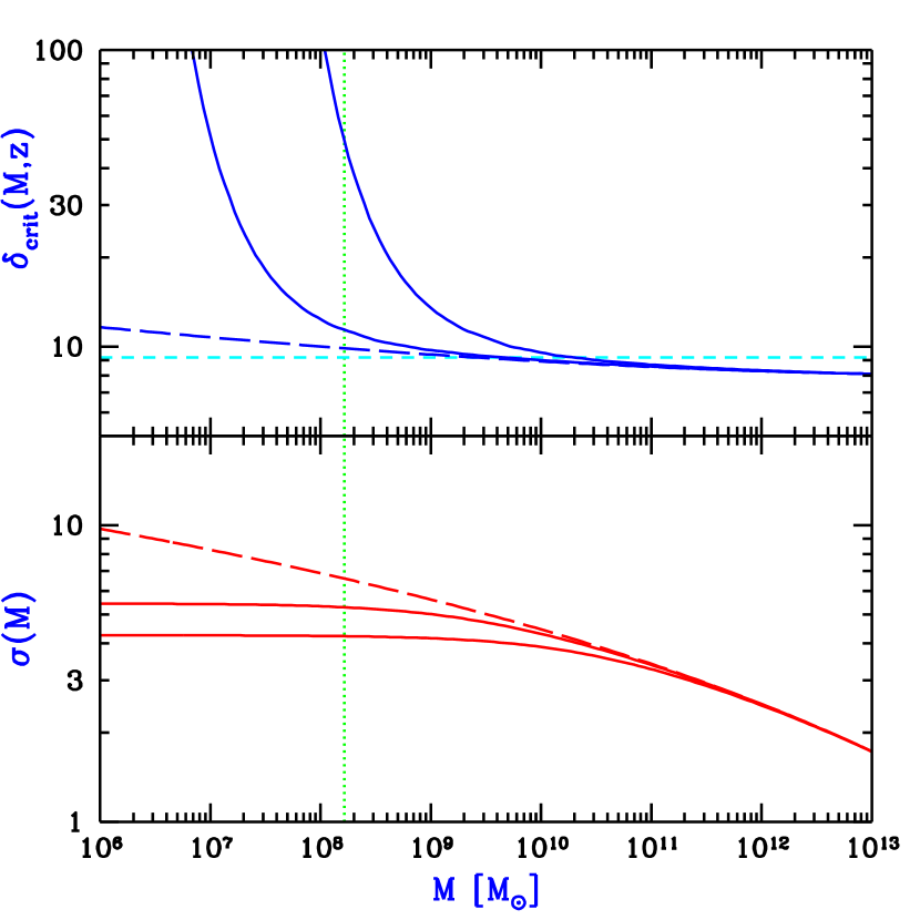
Figure 2: Halo formation in WDM, at $z=6$. In the top panel, we show the linear extrapolated overdensity $\delta_{c}(M,z)$ at the time of collapse, as a function of halo mass $M$. The solid curves show the cases of $m_{X}=1.5$ keV and $m_{X}=0.75$ keV, respectively from bottom to top. For comparison, we show the $\Lambda$CDM curve which includes the Sheth/Jenkins correction (long-dashed curve), and the mass-independent value given by spherical collapse in $\Lambda$CDM (short-dashed curve). In the bottom panel, we show the mass fluctuation $\sigma(M)$, based on the linearly-extrapolated power spectrum at matter-radiation equality. The solid curves illustrate the effect of the power spectrum cutoff in $\Lambda$WDM, for $m_{X}=1.5$ keV, and $m_{X}=0.75$ eV, respectively from top to bottom. Also shown for comparison is $\sigma(M)$ in $\Lambda$CDM (long-dashed curve). In both panels, the vertical dotted line shows the value of the lowest halo mass at $z=6$ in which gas can cool (see §3.3).

Like the other assumptions which enter into our semi-analytic model, our use of equation (16) is ultimately justifiable by comparing the final result to numerical simulations. Recently, Bode et al. (2000) performed simulations down to $z=1$ for $\Lambda$WDM with $m_{X}=0.35$ keV and $m_{X}=0.175$ keV, and compared them with a simulation of $\Lambda$CDM. In their Figure 9, Bode et al. (2000) show the halo mass function, in the form of the comoving number density $n(>M)$ of halos above mass $M$. We compare their results to our models in Figure 3. The model predictions which include only the suppression of the power spectrum (dotted lines) clearly do not produce enough suppression to match the simulations. The full model, which also accounts for the delay of halo collapse, still predicts less suppression than is seen in the simulations but matches more closely the simulated mass function over a range of scales for which the halo abundance is significantly suppressed compared to $\Lambda$CDM. The lowest-mass halos disappear in the $\Lambda$WDM models, while the simulations produce significant numbers of halos below $\sim 10^{10}M_{\odot}$ (for $m_{X}=0.35$ keV) and $\sim 10^{11}M_{\odot}$ (for $m_{X}=0.175$ keV). As noted by Bode et al. (2000), these halos do not form hierarchically, and thus are not accounted for in our models. These halos do not, however, affect our conclusions below about reionization. Such halos form by top-down “pancake” (actually ribbon) fragmentation at low redshift, and are not present in significant numbers at the high redshifts which are relevant for the reionization of the universe. In particular, the rare high-$\sigma$ peaks around which galaxies form at high redshift tend to be more nearly spherical and more centrally concentrated than low-$\sigma$ peaks (Bardeen et al., 1986). This should tend to reduce the importance of fragmentation at high redshift.

Even at low redshift, though, our models correctly predict the total mass fraction in halos, which is the quantity that is directly relevant to reionization. This successful prediction is shown in Figure 4, which presents differently the same data as in Figure 3. The quantity shown is the total mass fraction in halos up to halo mass $M$, as a function of $M$, except that we subtract out the mass fraction in halos below a mass of $1.5\times 10^{9}M_{\sun}$, which is roughly the minimum mass of halos which are well resolved in the simulations. As before, the good agreement is apparent for the $\Lambda$CDM model. In the WDM cases, the semi-analytic models give a much lower mass fraction than the simulations, in halos at the low-mass range, but when the mass is accumulated up to the highest-mass halos, the total mass fraction is in fact slightly higher in the models than in the simulations. Thus, in the simulations there is a shifting of mass from large halos to small halos, in that some regions that should collapse whole, according to the semi-analytic model, actually fragment and collapse as several sub-halos. The overall mass fraction in halos, however, is rather accurately reproduced by the model.

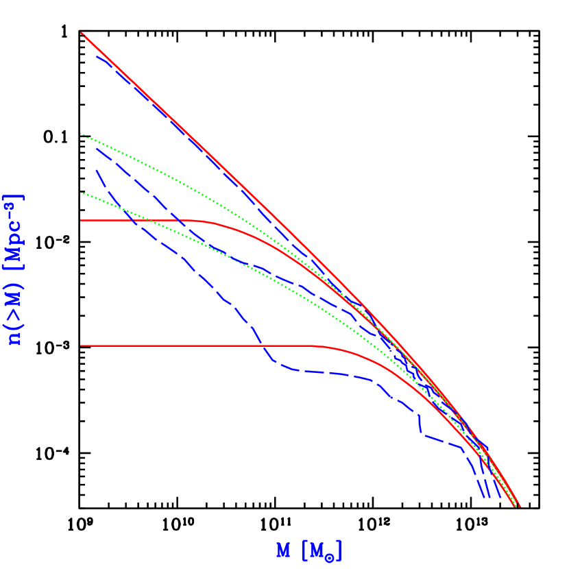
Figure 3: Numerical and semi-analytic halo mass functions at $z=1$ in $\Lambda$CDM and in $\Lambda$WDM. The curves show the comoving number density $n(>M)$ of halos above mass $M$. Solid lines show the semi-analytic calculation, and dashed lines show the results from numerical simulations by Bode et al. (2000). The three cases shown are, from top to bottom, $\Lambda$CDM, $m_{X}=0.35$ keV, and $m_{X}=0.175$ keV. The dotted lines show model predictions, for the two $\Lambda$WDM models, which include only the suppression of the power spectrum. The lowest-mass halos, those below $\sim 10^{10}M_{\odot}$ (for $m_{X}=0.35$ keV) or $\sim 10^{11}M_{\odot}$ (for $m_{X}=0.175$ keV), form in the simulations through fragmentation and are not accounted for in our models, but these halos do not affect our conclusions about reionization (see text). Note that the models shown in this figure use the cosmological parameters $\Omega_{\rm b}=0$ and $h=0.67$ for consistency with Bode et al. (2000).

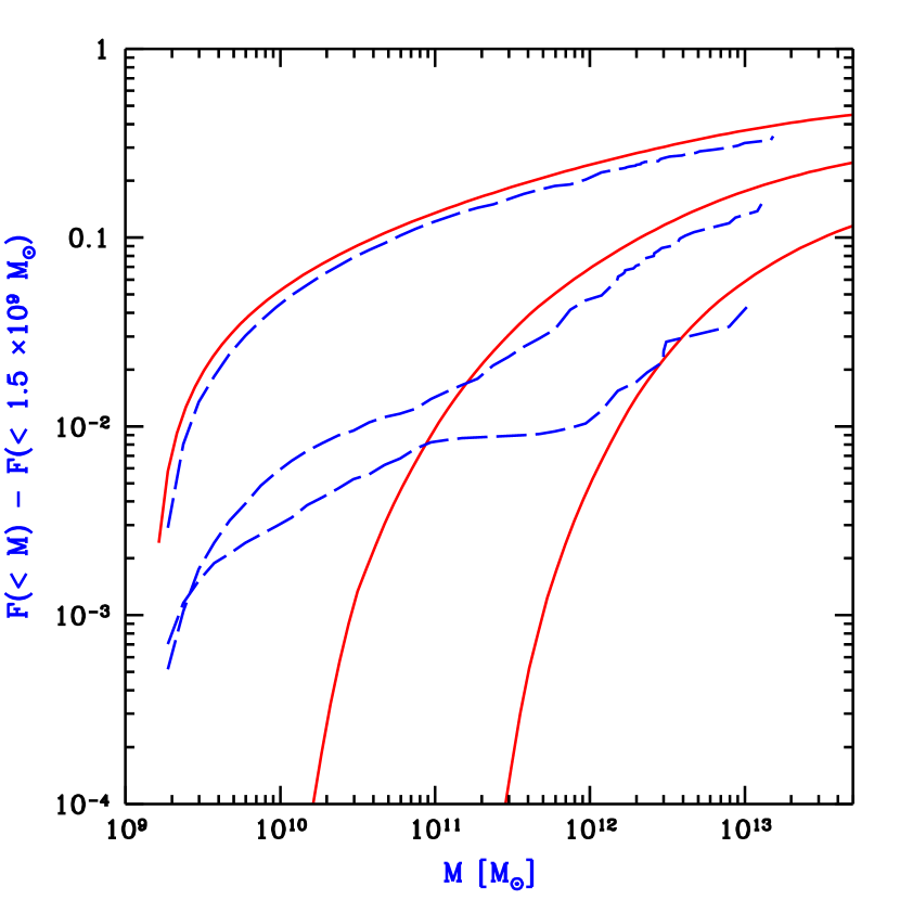
Figure 4: Numerical and semi-analytic halo mass fractions at $z=1$ in $\Lambda$CDM and in $\Lambda$WDM. The curves show the total mass fraction $F(<M)$ in halos up to mass $M$, with $F(<1.5\times 10^{9}M_{\sun})$ subtracted. Solid lines show the semi-analytic calculation, and dashed lines show the results from numerical simulations by Bode et al. (2000). The three cases shown are, from top to bottom, $\Lambda$CDM, $m_{X}=0.35$ keV, and $m_{X}=0.175$ keV. Note that the models shown in this figure use the cosmological parameters $\Omega_{\rm b}=0$ and $h=0.67$ for consistency with Bode et al. (2000).

We emphasize that the comparison of the semi-analytic mass function to the one derived from simulations must be considered preliminary. In the model, we have introduced a number of approximations, while the WDM simulations must also resolve a number of issues. For example, since some halos form through fragmentation, a clear comparison must be made of the results from different possible ways of identifying virialized halos in the simulations. In addition, sufficiently small scales are already weakly nonlinear at $z\sim 40$, and the neglect of non-linear effects can only be checked by making runs which start at a higher redshift.

As shown in §3.1, the collapse of a given halo must be followed from a very high redshift, near matter-radiation equality, in order for the full delay caused by the WDM velocities to be included. However, even though the numerical simulations are begun at $z\sim 40$, they do in fact include the effect of WDM velocities at higher redshift; the simulations use the appropriate initial power spectrum at the starting redshift, which implies, by the continuity equation, the correct initial mean velocity field (which gives the mean fluid velocity at every point). Therefore, the reduced power in the initial conditions also implies reduced infall velocities (through the Z’eldovich approximation), accounting for the cumulative dynamical effect of the WDM velocities at higher redshift. In our models, if we were only interested in the halo mass function at $z=1$, we could also start with the initial power spectrum at $z=40$, and use the ordinary $\delta_{\rm crit}(z)$, since any remaining WDM velocity dispersion would only affect extremely small mass scales [note the strong $z_{i}$-dependence of the effective Jeans mass, Eq. (10)]. Indeed, if random velocities are added to the simulations at $z=40$, their effect on $z<40$ dynamics is entirely negligible (Bode 2001, personal communication). Because the semi-analytic approach treats changes in $\sigma(M)$ differently from changes in $\delta_{\rm crit}(z,M)$, the prediction of the halo mass function at $z=1$ would give somewhat weaker suppression if we started at $z=40$ than if we start at equality. This points to a certain limitation or ambiguity in the semi-analytic approach, although we do find that the closest match to the numerical simulations (in terms of the total mass fraction in halos) is obtained by starting at equality. In any case, for reionization we are interested in the halo mass function at $z$ up to 30, and this forces us to choose a very high initial redshift.

Figure 5 shows our model predictions at $z=6$, in terms of the comoving halo mass function $dn/d\log(M)$ and the total mass fraction in halos above $M$, $F(>M)$. The figure shows the comparison for $\Lambda$CDM (solid line) and $\Lambda$WDM (dashed lines) with $m_{X}=1.5$ keV and $m_{X}=0.75$ keV (top to bottom). Reionization depends on the production rate of ionizing photons, which in turn depends on the mass fraction in halos in which gas cools and stars can form (for details see the following section). The value of the minimum mass for cooling at $z=6$, corresponding to a virial temperature of $T_{\rm vir}=10^{4}$K, is also shown in the figure (vertical dotted line). Clearly, in $\Lambda$WDM the mass fraction in galaxies is greatly reduced due to a sharp cutoff in the number density of halos below the cutoff mass. Note that for $m_{X}\lesssim 1.5$ keV the cooling mass is unimportant, i.e., even if the gas could cool in smaller halos, the effect would be negligible because the abundance of all halos below the cooling mass is severely reduced (see also Figure 7).

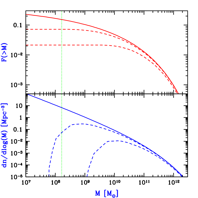
Figure 5: Semi-analytic halo mass functions at $z=6$ in $\Lambda$CDM and in WDM. The lower panel shows $|dn(>M)/d\log(M)|$, where $n(>M)$ is the comoving number density of halos above mass $M$. The upper panel shows the corresponding total mass fraction in halos above $M$, $F(>M)$. In both panels, solid lines are for $\Lambda$CDM and dashed lines for $\Lambda$WDM with $m_{X}=1.5$ keV and $m_{X}=0.75$ keV (top to bottom). Also shown is the minimum mass for cooling at $z=6$ (vertical dotted line).

3.3 Modeling Reionization

We model reionization using a simplified semi-analytic scheme, following Haiman & Loeb (1998). Although this approach does not capture all the details of the reionization process (see, e.g., Gnedin, 2000), it is adequate for our present purpose of estimating the required overall ionizing-photon budget. We assume that dark halos form at a rate $d^{2}n/(dM\,dt)$, where $dn/dM$ is the halo mass function. When a halo collapses, it converts a fraction of its baryonic mass into either stars or a central black hole (BH). Each new halo then turns into an ionizing source, and creates an expanding H II region. The evolution of the proper volume $V_{i}$ of a spherical H II /H I ionization front for a time-dependent source is governed by the equation

$$\frac{dV_{i}}{dt}=3H(z)V_{i}+\frac{\dot{N}_{\rm\gamma}(t)}{\bar{n}_{\rm H}}-1.079\,C\,\bar{n}_{\rm H}\,\alpha_{B}V_{i},$$ (17)

where $t$ is the age of the source, $H(z)$ is the Hubble constant, $\bar{n}_{\rm H}$ is the neutral hydrogen number density in the smooth IGM at redshift $z$, $\dot{N}_{\rm\gamma}(t)$ is the production rate of ionizing photons, $\alpha_{\rm B}=2.6\times 10^{-13}~{}{\rm cm^{3}~{}s^{-1}}$ is the recombination coefficient of neutral hydrogen to its excited states at $T=10^{4}$K, and $C\equiv\langle n_{\rm H}^{2}\rangle/\bar{n}_{\rm H}^{2}$ is the mean (volume-weighted) clumping factor of ionized gas within $V_{i}$ (i.e., excluding any dense, self-shielded neutral clumps). In the recombination term, we have included a factor of 1.079 due to the additional free electrons produced if helium is singly ionized, as expected in the case of a reionization dominated by stars. The first term in equation (17) accounts for the Hubble expansion, the second term accounts for ionizations by newly produced photons, and the last term describes recombinations (Shapiro & Giroux, 1987; Haiman & Loeb, 1997). The solution of this equation yields the proper  ionized volume per source, and a summation over all sources provides the total ionized volume within the IGM.

We compute the production rate of ionizing photons for a stellar population with a Scalo (1998) IMF (initial mass function) undergoing a burst of star formation at a metallicity equal to $2\%$ of the solar value (Bruzual & Charlot, 1996). We find that the rate is well approximated by

$$\dot{N}_{\rm\gamma}(t)=\left\{\matrix{\dot{N}_{0}\hfill&(t\leq 10^{6.5}~{}{\rm yr})\hfill\cr\dot{N}_{0}(t/10^{6.5}{\rm yr})^{-4.5}\hfill&(t>10^{6.5}~{}{\rm yr})\hfill,\cr}\right.$$ (18)

where $\dot{N}_{0}=3.7\times 10^{46}~{}{\rm s^{-1}~{}M_{\odot}^{-1}}$ (per ${\rm M_{\odot}}$ of stellar mass). Over the lifetime of the population, this produces $\approx 4000$ ionizing photons per stellar proton. We also assume a typical star formation efficiency of $f_{*}\equiv M_{\rm stars}/(\Omega_{\rm b}M_{\rm halo}/\Omega_{0})=10\%$, consistent with the observed star formation rate at $z\sim 3$–4 (e.g., Barkana & Loeb, 2000) and with observations of the metallicity of the Ly$\alpha$ forest at $z=3$ (Haiman & Loeb, 1997); this efficiency implies that $\approx 7.2\times 10^{58}$ ionizing photons are produced per ${\rm M_{\odot}}$ of total (dark matter + gas) halo mass. We assume further that the escape fraction of ionizing photons is $f_{\rm esc}=10\%$, based on observational estimates for present-day galaxies (e.g., Bland-Hawthorn & Maloney, 1999; Hurwitz, Jelinsky, & Dixon, 1997, but note Steidel, Pettini, & Adelberger 2001). Since the star formation efficiency and the escape fraction always appear as a product, we define the parameter $\epsilon_{*}\equiv f_{*}f_{\rm esc}$ to parameterize the efficiency of ionizing photon injection into the IGM. At present, the best direct observational constraint on $\epsilon_{*}$ is provided by measurements of the mean ionizing flux at $z=3$ based on the proximity effect of quasars. We discuss this further in §4.2; we show there that these measurements imply $\epsilon_{*}=0.01$, with about a factor of 2 uncertainty.

The analogous $\dot{N}_{\rm\gamma}(t)$ from gas accretion onto a quasar BH is not available from an ab-initio theory. However, it can be derived (for details see Haiman & Loeb, 1998) by postulating a BH formation efficiency ($\epsilon_{Q}\equiv M_{\rm bh}/M_{\rm halo}$), adopting an average quasar spectrum (e.g., Elvis et al., 1994), and finding the quasar light-curve that fits the luminosity function of optical quasars (e.g., Pei, 1995). Note that the Elvis et al. (1994) spectral template we adopt ($F_{\nu}\sim\nu^{-1}$) is somewhat harder than the template ($F_{\nu}\sim\nu^{-1.8}$) of, e.g., Zheng et al. (1998), which would therefore produce fewer ionizing photons. For a constant ratio $\epsilon_{Q}=6\times 10^{-4}$ which is based on observations (Magorrian et al., 1998), the above procedure results in $\dot{N}_{\rm\gamma}(t)\approx 6.6\times 10^{47}\exp(-t/10^{6}{\rm yr})~{}{\rm s^{-1}}$, yielding approximately $17,000$ ionizing photons per baryon in the BH; or alternatively $\approx 1.2\times 10^{58}$ per ${\rm M_{\odot}}$ of total halo mass. Below we focus on stellar reionization, and we simply note that quasar BH’s would produce $\approx 6$ times fewer ionizing photons, but their escape fraction may compensate by being substantially higher than for stars (e.g., Wood & Loeb, 2000).

In order to compute the expansion rate of the H II regions, we must specify the clumping factor $C$ of ionized gas in Eq. (17). Here we simply assume a constant value of $C=10$. For $\Lambda$CDM this is a very conservative value for the epoch of reionization; since the early ionizing sources form in the highest-density regions, the clumping factor reaches values as high as $\approx 100$ in three-dimensional simulations (Gnedin, 2000). Note, however, that this value for clumping accounts only for absorption by gas at the highest resolvable density in the simulation. A higher-resolution simulation would have higher-density gas clumps and — depending on the geometry of those clumps — a higher or possibly lower clumping factor than the low-resolution simulation. The clumping factor should also be lower in the case of $\Lambda$WDM, where clumping in the dark matter is smoothed out on small scales. The precise effect on the gas clumping factor can only be determined with numerical simulations or with detailed models. Below we examine how our results change when other constant values ($C=1,30$) are assumed.

Finally, to compute the total ionized fraction $F_{\rm H\,II}$, we convolve the solution of equation (17) with the total cosmological star formation rate, by

$$F_{\rm H\,II}(z)=\epsilon_{*}\int_{0}^{t(z)}dt^{\prime}\dot{\rho}_{g}(t^{\prime}){\tilde{V}}_{\rm H\,II}(t^{\prime},t).$$ (19)

Here $t(z)$ is the cosmic time at redshift $z$, $\rho_{g}(t)=F_{\rm col}\Omega_{\rm b}\rho_{\rm crit}$ is the total collapsed gas density (mass per unit comoving volume), $\rho_{\rm crit}$ is the present-day critical density, and ${\tilde{V}}_{\rm H\,II}(t^{\prime},t)$ is the comoving ionized volume per unit stellar mass at $t$ for a source which emitted at time $t^{\prime}$. The collapsed fraction of baryons is evaluated as $F_{\rm col}(z)=F(>M_{\rm min}(z))$, where the mass fraction $F(>M|z)$ in halos above mass $M$ at redshift $z$ is calculated as in §3.2. The minimum mass $M_{\rm min}(z)$ is chosen by requiring efficient cooling; we assume that the gas within halos smaller than $M_{\rm min}(z)$ cannot turn into stars. In the metal-deficient primordial gas, the critical mass $M_{\rm min}(z)$ for cooling corresponds to a virial temperature of $T_{\rm vir}\approx 10^{4}\,$K. Unless the earliest UV sources produce significant X-rays, which then catalyze the formation of molecular hydrogen, it is unlikely that smaller halos can contribute to reionization (see Haiman, Abel & Rees, 2000). Furthermore, for the ranges of WDM particle masses we explore here, the abundance of such small halos is severely suppressed, making their ability to form stars irrelevant for the constraints we derive (see also Figures 5 and 7).

Based on the spherical collapse simulations (§3.1), we find that the non-zero velocity of WDM causes a small change in the $T_{\rm vir}-M_{\rm halo}$ relation. We find, however, that this effect is almost negligible. Although the collapse of halos is delayed relative to their evolution in a CDM universe, once a WDM halo does collapse, it has nearly the same overdensity relative to the universe at the collapse redshift as it would have in the CDM case (see the discussion of Figure 1). Indeed, halos with the same mass collapsing at the same redshift look nearly indistinguishable in the WDM and CDM runs; the main difference is that the density fluctuations producing the WDM halos had a larger initial amplitude. This suggests that WDM can greatly affect the abundance of halos of a given mass without significantly affecting their virial overdensity. Note, however, that in the hierarchical-merging picture WDM may still affect the inner profiles and the substructure of halos. Material which makes up the dense core region and some of the substructure within a given CDM halo originates in small halos at higher redshift, which are later accreted. If WDM suppresses the abundance of these high-redshift halos it will affect the inner structure of later halos (see, e.g., Subramanian, Cen, & Ostriker, 2000).

4 Results and Discussion

4.1 A Constraint from the Quasar Black Hole in SDSS 1044-1215.

Before describing the constraint on the WDM mass we obtain from reionization, we first mention a more direct, albeit somewhat weaker constraint. The quasar SDSS 1044-1215 discovered by the SDSS at redshift $z=5.8$ has an apparent $z^{\prime}$ magnitude of $\approx 19.2$. Under the assumption that this object is neither beamed nor lensed, and shining at the Eddington luminosity, the mass of the central BH is inferred to be $M_{\rm bh}=3.4\times 10^{9}~{}{\rm M_{\odot}}$ (see Fan et al. 2000 and Haiman & Loeb 2000 for discussions of how the mass was derived). If this supermassive BH grew exponentially by accretion onto a smaller seed BH, the required time for growth is $\ln(3.4\times 10^{9}M_{\odot}/M_{\rm seed})\approx 20$ $e$-folding times for stellar seeds, where $M_{\rm seed}$ is the mass of the seed. The natural $e$-folding timescale is the Eddington time, or $4\times 10^{7}(\epsilon/0.1)~{}{\rm yr}$, where $\epsilon$ is the radiative efficiency of accretion. Assuming $\epsilon=0.1$, and a seed mass of either $M_{\rm seed}=10~{}{\rm M_{\odot}}$ or $M_{\rm seed}=100~{}{\rm M_{\odot}}$, we find that the seed had to be present, and start growing by a redshift of $z=20$, or $z=15$, respectively.

The required presence of a seed by a redshift of $z=20$ or $z=15$ implies that a halo must have collapsed by this redshift within the comoving volume probed by the SDSS survey to find SDSS 1044-1215. This comoving volume is approximately 5 Gpc³, enclosed by a solid angle of 600 deg² and a redshift bin $\Delta z=1$ at redshift $z=5.8$ in our $\Lambda$CDM cosmology. The appropriate choice for the size of the redshift bin depends on the parameters of the set of broad-band filters used in the SDSS. In particular, the Sloan $z^{\prime}$ filter that is used to find high-redshift quasars is centered at 9130Åwith a width of 1900Å, corresponding to sensitivity over the redshift interval $5.3<z<6.3$. In Figure 6, we show the cumulative mass functions, i.e., the abundance of all halos with masses exceeding $M$, at $z=20$ and $z=15$. The dashed curves show the mass function in the $\Lambda$CDM cosmology, while the solid curves correspond to mass functions in $\Lambda$WDM models with $m_{X}=1.25,1.00,0.75$, and $0.50$ keV, respectively from top to bottom. In each panel of Figure 6, the horizontal dotted line corresponds to the abundance of one halo per 5 Gpc³, the requirement for a halo to host a seed for SDSS 1044-1215. As the figure shows, for a seed mass of $M_{\rm seed}=100~{}{\rm M_{\odot}}$, the required halo abundance at $z=15$ results in the limit $m_{X}\gtrsim 0.47$ keV (or $v_{\rm rms,0}\lesssim 0.119$ km/s). Similarly, for a seed mass of $M_{\rm seed}=10~{}{\rm M_{\odot}}$, the required halo abundance at $z=20$ yields the constraint $m_{X}\gtrsim 0.79$ keV (or $v_{\rm rms,0}\lesssim 0.059$ km/s). These limits would strengthen with the discovery of more than one bright quasar in the $5.3<z<6.3$ redshift range. E.g., we find that a total of four objects, similar in brightness to SDSS 1044-1215, would imply $m_{X}\gtrsim 0.51$ and $m_{X}\gtrsim 0.85$ for the high and low seed mass, respectively.

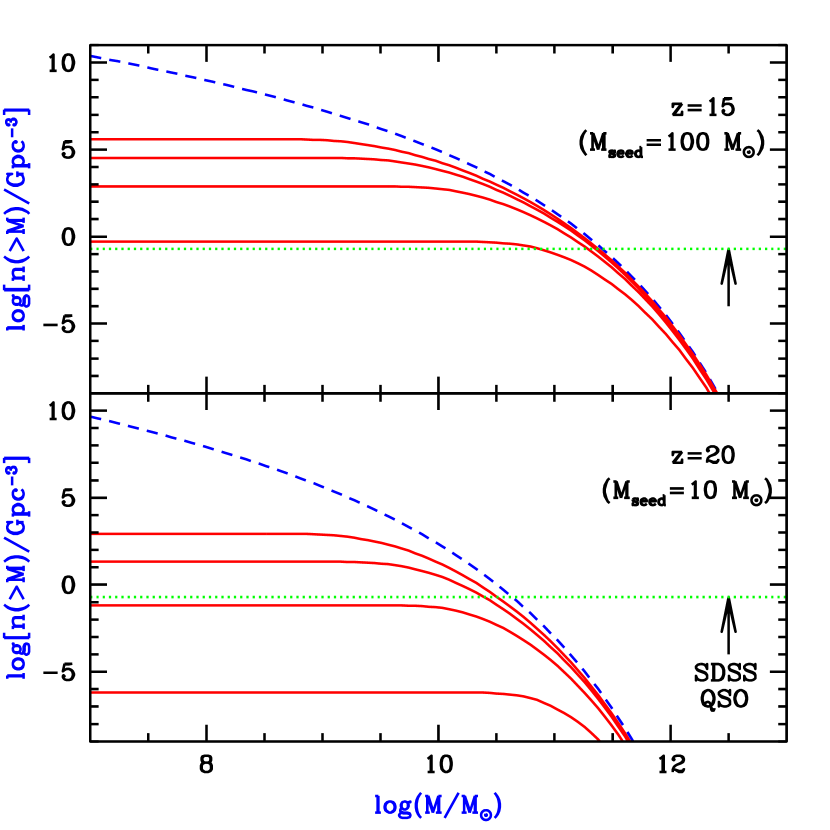
Figure 6: The cumulative mass function of dark halos at two different redshifts ($z=15$, upper panel; $z=20$, lower panel). The dashed curves show the mass function in the $\Lambda$CDM cosmology, while the solid curves correspond to mass functions in $\Lambda$WDM models with $m_{X}=1.25,1.00,0.75$, and $0.50$ keV, respectively from top to bottom. The horizontal dotted line in each panel corresponds to the minimum abundance of one halo per 5 Gpc³, required for a host halo to harbor a seed for the supermassive BH inferred to power the quasar SDSS 1044-1215.

These constraints are somewhat weaker than those we find from reionization below. Nevertheless, they are comparable to the existing limits summarized in the Introduction. This type of constraint would strengthen significantly if the time-averaged mass accretion rate of BHs was low. In the above estimates, we assumed that the fueling rate is sufficient to continuously maintain a luminosity near the Eddington luminosity (and that the growth of the holes is limited by this luminosity). However, as suggested by Ciotti & Ostriker (1997, 2000), this may not be the case, if the accretion is episodic because the inflow of gas is quenched by heating of the surrounding gas due to Compton scattering of the high-energy photons emitted by the central quasar. On the other hand, a lower radiative efficiency would imply that the accretion rate could be higher than we have assumed, without exceeding the Eddington luminosity. However, by comparing the total mass in BHs at the centers of nearby galaxies with the total light output of quasars, we know that the average radiative efficiency of quasars over their lifetimes cannot be much lower than $10\%$, at least statistically, for the quasar population as a whole (Soltan, 1982; Barger et al., 2001). We note further that the simple limit on the halo abundance we derived here can likely be improved, since not all halos present at $z=20$ or $z=15$ can plausibly host a seed for the BH in SDSS 1044-1215. Indeed, the host-halo of the SDSS quasar is likely very massive ($M\gg 10^{10}~{}{\rm M_{\odot}}$), and among the high-redshift halos, only those that merge into such large halos by $z=5.8$ can serve as hosts for the seed BH. A full treatment of this problem requires the knowledge of the conditional mass function in $\Lambda$WDM cosmologies, and this is not investigated further in the present work (but see Haiman & Loeb 2000 for a parallel discussion in usual $\Lambda$CDM cosmologies).

4.2 Constraints from Reionization.

In this section, we derive the reionization history in universes dominated by WDM with various particle masses, given the approximate theory presented in § 3 above. The main differences in the reionization histories arise simply from the different collapsed baryon fractions $F_{\rm col}$ when different particle masses are assumed. In the bottom panel of Figure 7 we show the collapsed fraction when the assumed WDM particle mass is between 0.25 keV and 3 keV, in increments of 0.25 keV (dotted curves, bottom to top). The solid curve highlights the particular case of $m_{X}=1.25$ keV, which is near the limit from reionization with our standard assumptions (see below). The dashed curve shows the collapsed fraction in a $\Lambda$CDM universe. In each case, $F_{\rm col}$ declines sharply at high redshifts; lower particle masses result in more significant suppression of the collapsed fraction. While the bottom panel of Figure 7 assumes our standard value of $10^{4}$K for the minimum halo virial temperature required for cooling, the top panel compares the case of a minimum virial temperature of $10^{2}$K, which corresponds to efficient cooling with molecular hydrogen. Clearly, although the precise cooling threshold is crucial for $\Lambda$CDM, the halo suppression due to WDM makes halos below a virial temperature of $10^{4}$K unimportant for the entire range of $\Lambda$WDM models which we consider. This is especially true at the highest redshifts, where (for a fixed virial temperature) the minimum cooling mass is relatively small.

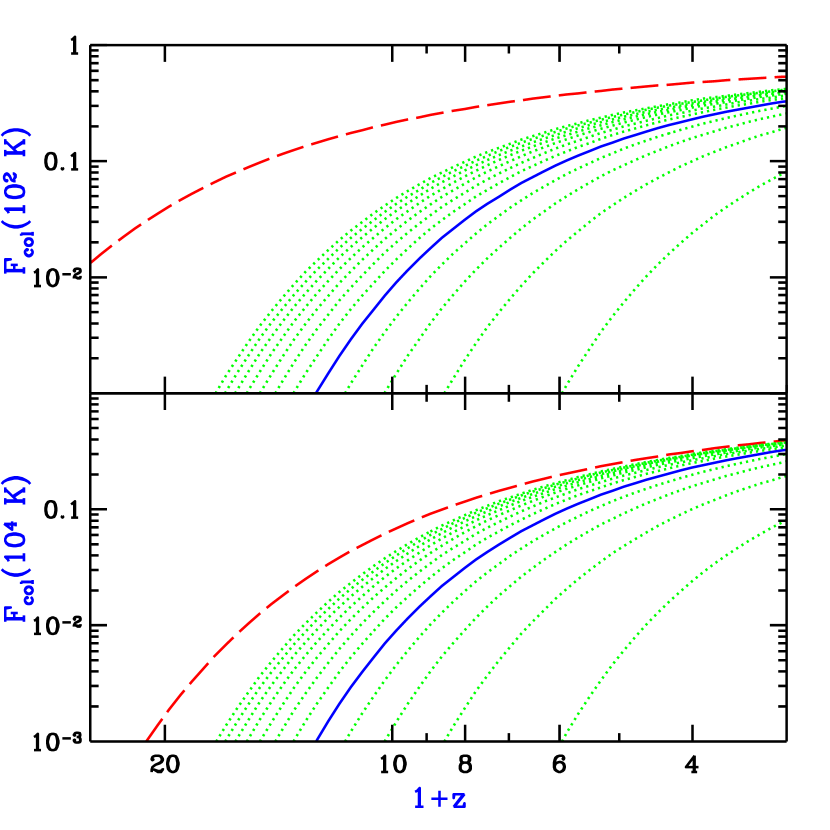
Figure 7: The fraction of baryons collapsed in halos, as a function of redshift $z$, for different WDM particle masses. The bottom panel assumes a minimum halo virial temperature of $10^{4}$K, which is our standard case and corresponds to efficient atomic cooling; the top panel shows the case of a virial temperature of $10^{2}$K, which corresponds to efficient cooling in the presence of a significant abundance of molecular hydrogen. In both panels, the dotted curves show WDM particles with masses between 0.25 keV and 3 keV, in increments of 0.25 keV (bottom to top). The $m_{X}=1.25$ keV case (which is close to the limit we derive below) is highlighted with a solid curve. The dashed curve shows the collapsed fraction in a $\Lambda$CDM universe. Comparing the two panels shows that the reionization histories in the $\Lambda$CDM models are sensitive to the assumed minimum cutoff mass, but this sensitivity disappears in the $\Lambda$WDM models.

Once the collapsed fraction is known in a given cosmology, the filling factor of ionized regions, $F_{\rm H\,II}$ follows as discussed in §3.3 above. As an example, in Figure 8, we show the evolution of $F_{\rm H\,II}$ in our standard model ($C=10,\epsilon_{*}=0.01$), assuming a WDM particle mass of 1.25 keV ($v_{\rm rms,0}=0.031$ km/s; solid curve). For reference, the short-dashed curve shows the filling factor in the $\Lambda$CDM model. As discussed above, WDM reduces the collapsed fraction of baryons due to two distinct reasons: first because the power spectrum is suppressed at low masses; and second, because the collapse of each low-mass halo near and below the critical cutoff mass is delayed. In order to assess these effects separately, in Figure 8 we show the evolution of the filling factor when the power spectrum is suppressed, but the collapse of each halo is kept the same as in $\Lambda$CDM (dotted curve); and conversely, when the collapse of each halo is delayed by the WDM, but the power spectrum is kept the same as in $\Lambda$CDM (long-dashed curve). This pair of curves reveals that both effects lead to a substantial reduction of the total amount of collapsed gas. The two effects are comparable at high redshift, but the power spectrum cutoff is dominant at reionization. When both effects are included, the filling factor reaches a value of unity only at a redshift of $z=6.0$, as opposed to a redshift of $z\approx 7.4$ in the corresponding $\Lambda$CDM case.

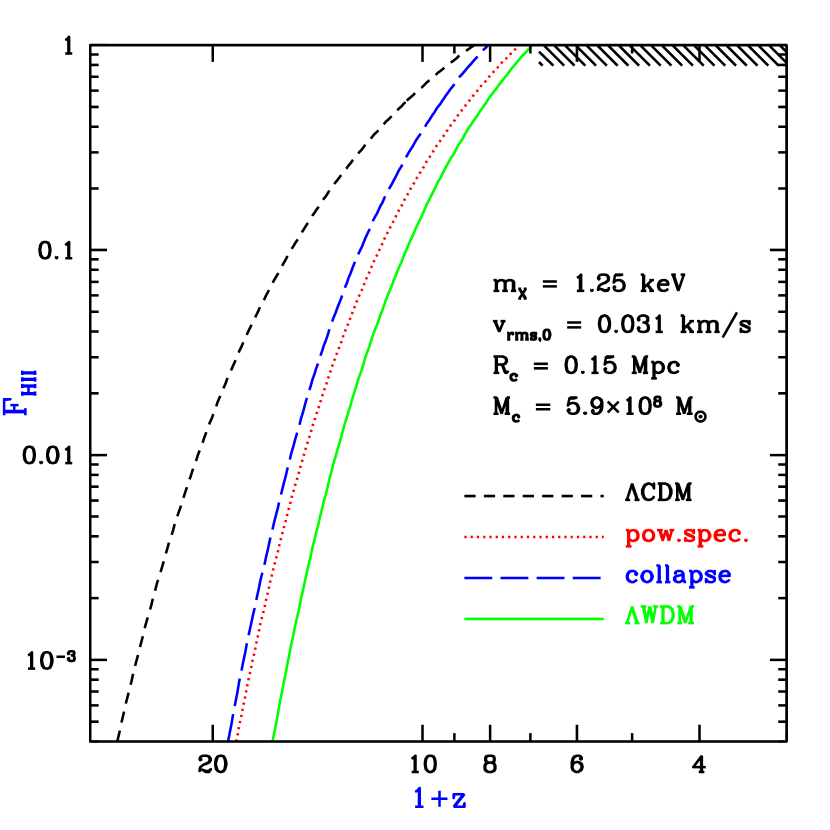
Figure 8: The filling factor of ionized hydrogen, $F_{\rm H\,II}$, as a function of redshift $z$ in our standard model ($C=10,\epsilon_{*}=0.01$). The uppermost (short dashed) curve corresponds to $\Lambda$CDM, and the lowest (solid) curve to a WDM particle mass of $m_{X}=1.25$ keV. The middle pair of curves shows the separate contributions to the delay in reionization from the delay in the collapse of individual halos (long dashed curve) and from the suppression of the power spectrum (dotted curve). The shaded region in the upper right corner indicates the requirement $z_{\rm reion}>5.8$. Also given in the figure are the values of the corresponding velocity $v_{\rm rms,0}$ as well as the cutoff scale $R_{c}$ and mass $M_{c}$, defined using the $z=0$ power spectrum.

The generic trend demonstrated in Figure 8 holds when different particle masses are assumed: the delayed collapse of individual halos, and the suppression of the power spectrum both contribute to a delay in the reionization epoch, with the latter effect dominating. As can be expected from Figure 7, the reionization redshift is a strong function of the assumed WDM particle mass. The current best lower limit on the reionization redshift is $z=5.8$, inferred from the spectrum of a bright quasar found at this redshift in the Sloan Digital Sky Survey (SDSS, Fan et al., 2000). In our models, we define reionization to occur at the redshift when the filling factor formally reaches unity. Although this choice is somewhat arbitrary, it is likely a conservative assumption, since even after the entire IGM is reionized, its opacity remains very large for some time until the neutral hydrogen fraction drops to $\lesssim 10^{-6}$. We compute the evolution of $F_{\rm H\,II}$ for various WDM masses $m_{X}$ and obtain the reionization redshift under this definition.

Figure 9 shows the resulting value of $z_{\rm reion}$ as a function of WDM particle mass in our models. The thick solid curve corresponds to our standard model, and results in a limit of 1.2 keV on the WDM particle mass (which corresponds to $v_{\rm rms,0}\leq 0.033$ km/s). In order to assess the robustness of the limit on the WDM particle mass, in Figure 9 we also show results for variations away from our standard parameters values. The top and middle solid curves assume $\epsilon_{*}=1$ and $\epsilon_{*}=0.1$, respectively, and yield limits of 0.28 and 0.43 keV. For each of the models represented by the three solid curves (which all assume a clumping factor $C=10$), we also show corresponding results when $C=1$ (upper, dotted curve), and when $C=30$ (lower, dashed curve). We regard the upper-most triplet of models as extreme cases, where the star formation efficiency and escape fraction are both adjusted to their highest possible values. An exception to this is the stellar IMF: if it is heavily biased towards high-mass stars, the ionizing photon yields can be substantially increased. Note, however, that even in the most extreme models, the constraint $E>0.25$ keV follows.

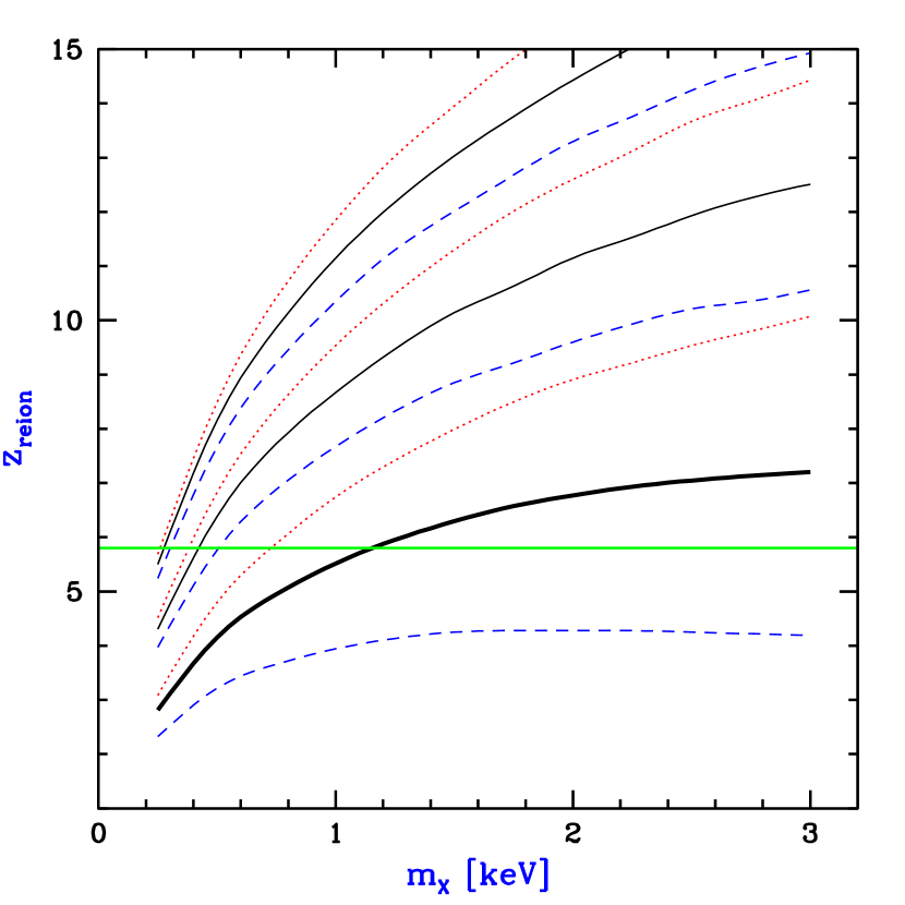
Figure 9: Reionization redshift as a function of WDM particle mass. Our standard model, which adopts standard values for the star-formation efficiency, escape fraction, and stellar IMF, is shown by the thick solid line. The three solid curves show models with the same clumping factor ($C=10$) but different ionization efficiencies ($\epsilon_{*}=0.01,0.1,1$, bottom to top). The three dotted curves correspond to the same models except with $C=1$; similarly, the three dashed curves correspond to these models except with $C=30$. In our standard model, the requirement that $z_{\rm reion}>5.8$ limits the WDM particle mass to be $E>1.2$ keV; in the most extreme model, the limit is lowered to $E\gtrsim 0.25$ keV.

An interesting feature of Figure 9 is the strong dependence of the limiting particle mass on the assumed limit on the reionization redshift. Although the redshift limit is currently $z=5.8$, if $\Lambda$CDM is correct, future observations could soon increase this redshift and tighten the constraint on WDM. If the limit is increased beyond $z=7.4$, it would rule out the model with our standard parameters, even in $\Lambda$CDM. The Next Generation Space Telescope  (NGST ) could push the redshift limit to $z>10$, which would greatly constrain $\Lambda$WDM even with reionization parameters stretched to values that appear unlikely at present. Also, models of cosmological parameter estimation from future CMB measurements (Eisenstein, Hu, & Tegmark, 1999; Zaldarriaga, Spergel, & Seljak, 1997) suggest that the reionization redshift should be easily measurable with the Planck satellite, and the polarization signature of reionization is likely detectable even with the upcoming MAP satellite.

It is useful to assess the individual contributions of the power spectrum cutoff, and delayed collapse of halos, to these limits on the WDM particle mass. As an example, in models with a constant clumping of $C=10$, Figure 9 reveals the limits of 0.28, 0.43, and 1.17 keV for $\epsilon_{*}=1$, 0.1, and 0.01, respectively. If the power spectrum cutoff were ignored, these limits would change to 0.17, 0.29, and 0.71 keV; similarly, if the effect of the WDM on the collapse of halos were ignored, the limits would be 0.15, 0.29, and 0.98 keV. As before, the cutoff plays a larger role than halo dynamics. Note that the constraints that we obtain when only the cutoff is included would also apply to any modification of the $\Lambda$CDM model in which the power spectrum is sharply cut off below the scale $R_{c}$ given by equation (4).

As mentioned in §3.3, we can normalize the parameter $\epsilon_{*}$ in our models by computing the background flux produced at redshift $z=3$ and comparing with observations. The measured value at $z\sim 3$ from the proximity effect is around $J_{21}=0.7$, i.e., the proper intensity is $J=0.7\times 10^{-21}~{}{\rm erg~{}s^{-1}~{}cm^{-2}~{}Hz^{-1}~{}sr^{-1}}$ (Scott et al. 2000; see also Bajtlik, Duncan, & Ostriker 1988 for the basic measurement method). The observed flux at redshift $z<z_{\rm reion}$ and frequency $\nu$, in units of ${\rm erg~{}cm^{-2}~{}s^{-1}~{}Hz^{-1}~{}sr^{-1}}$ is given by (e.g., Peebles, 1993)

$$J(\nu,z)=\frac{c}{4\pi}\int_{z}^{z_{\rm reion}}dz^{\prime}\frac{dt}{dz^{\prime}}\,j^{*}_{\nu_{z}^{\prime}}(z^{\prime})\left(\frac{1+z}{1+z^{\prime}}\right)^{3}\exp\{-\tau(z,z^{\prime},\nu)\},$$ (20)

where $c\,dt/dz$ is the cosmological line element per unit redshift, $\nu_{z}^{\prime}=\nu(1+z^{\prime})/(1+z)$ is the frequency appropriate for photons emitted at redshift $z^{\prime}$, $j^{*}$ is the proper emission coefficient in units of ${\rm erg~{}cm^{-3}~{}s^{-1}~{}Hz^{-1}}$, and $\tau(z,z^{\prime},\nu)$ is the effective optical depth between redshifts $z$ and $z^{\prime}$ for a photon emitted at frequency $\nu_{z}^{\prime}$ at $z^{\prime}$. Note that we impose the upper limit $z_{\rm reion}$ on the integral, since photons emitted prior to this redshift are used to reionize the universe, and do not contribute to the background flux. Madau (1995) calculated the optical depth $\tau(z,z^{\prime},\nu)$ based on the distribution of Ly$\alpha$ absorption systems in redshift and hydrogen column density; we adopt this optical depth but with a factor of 0.6 correction, for consistency both with more recent observations of the distribution of Ly$\alpha$ absorption systems (Fardall et al., 1998) and with a recent measurement of absorption in quasar spectra at $z=3.4$ (Steidel et al., 2001). In our models, the stellar emission coefficient is given by a sum of the instantaneous emission from all the stars (of different ages) present at $z$,

$$j^{*}_{\nu}(z)=\epsilon_{*}\Omega_{\rm b}\rho_{\rm c0}(1+z)^{3}\int_{z}^{\infty}dz^{\prime}\frac{dF_{\rm col}}{dz^{\prime}}\epsilon^{\rm star\,}[\nu(1+z^{\prime}),t_{z,z^{\prime}}],$$ (21)

where $\rho_{\rm c0}$ is the current critical density of the universe, $t_{z,z^{\prime}}$ is the time interval between the redshift $z^{\prime}$ at which a star was born, and the redshift $z$, and $\epsilon^{\rm star\,}(\nu,t)$ is the composite physical emissivity (in ${\rm erg~{}s^{-1}~{}Hz^{-1}~{}M_{\odot}^{-1}}$) of a population of stars with our adopted IMF (Scalo, 1998), as given by the Bruzual & Charlot (1996) model at time $t$ after an initial starburst. In calculating $dF_{\rm col}/dz^{\prime}$ in equation (21) we include the suppression of the formation of dwarf galaxies after reionization (e.g., Efstathiou, 1992; Thoul & Weinberg, 1996; Navarro & Steinmetz, 1997), approximated here as a sharp cutoff at a halo circular velocity of 40 km/s. The severe opacity faced by ionizing photons from high redshifts implies that $J_{21}$ at $z=3$ essentially fixes the star formation rate at $z=3$. For different WDM masses $m_{X}$, all with the same efficiency $\epsilon_{*}$, the cosmic star formation rate differs greatly at high redshift but by $z=3$ is fairly insensitive to $m_{X}$.

The measured value of $J_{21}$ is highly uncertain and may be about a factor of 2 higher or lower. It is also, in fact, averaged over $z=2$–4. In applying this measurement to our models, we must consider the possibility that different source populations dominate the ionizing intensity at $z\sim 3$ and at reionization. Indeed, a decrease with redshift in the contribution of quasars to the ionizing background around $z\sim 3$ is suggested by observations of variable He II opacity (e.g., Heap et al., 2000; Anderson et al., 1999), evolution in the Si IV/C IV ratio in Ly$\alpha$ absorption systems (Songaila, 1998; Boksenberg et al., 1998), and the relatively high temperature of the IGM at $z\sim 3$ (Ricotti et al., 2000; Schaye et al., 2000; Bryan & Machacek, 2000; McDonald et al., 2000b). If the trend indicated by these observations continues to higher redshift, it justifies our reionization models which include only stellar emission. However, the observed $J_{21}$ at $z=2$–4 may include a significant contribution from quasars. Indeed, the value of $J_{21}$ derived from the proximity effect is consistent with the ionizing flux expected from quasars (Haardt & Madau, 1996). Thus, our $m_{X}=1.2$ keV model with standard parameters, which reionizes at $z=5.8$, is fully consistent with observations of the proximity effect; in the simple calculation based on equations (20) & (21) above it yields a flux of $J_{21}=0.36$ at $z=3$, consistent with the measured value of $J_{21}=0.7$ if quasars and stars make a comparable contribution to the observed $J_{21}$. Given the uncertainties, however, we estimate a range of possible normalizations of our model by allowing a stellar contribution to $J_{21}$ that is higher or lower by a factor of 2. At the lower end, if $J_{21}<0.22$ then even the $\Lambda$CDM model does not reionize by $z=5.8$. At the higher end, if stars contribute a $J_{21}=0.72$ at $z=3$ then our limit on WDM weakens to $m_{X}>0.75$ keV.

Although normalizing our models to a fixed value of $J_{21}$ adds a direct observational constraint, the computation of the flux in our models depends on the assumption that $\epsilon_{*}$ does not evolve with redshift. We also note here an observational result which may conflict with those mentioned above. Steidel et al. (2001) have reported a preliminary detection of significant Lyman continuum flux in a composite spectrum of 29 Lyman break galaxies at $z=3.4$. The observed flux level implies a large escape fraction of ionizing radiation, and may be inconsistent with the spectral break at 912Å expected from stars with the IMF that our models assume. If the Steidel et al. (2001) results are representative of the galaxy population as a whole, then galaxies contribute $\sim 5$ times more ionizing flux than quasars to the background flux at $z=3.4$. On the other hand, Heckman et al. (2001) applied a different method based on interstellar absorption lines and found a very low $f_{\rm esc}<6\%$ in several local starburst galaxies and one such galaxy at $z=2.7$. Further measurements are needed to settle this issue, especially cross-checks where different methods are applied to the same galaxies. In addition, measurements of the probability distribution of transmitted flux in the Lyman-$\alpha$ forest of quasar absorption lines also suggest a low ionizing background, $J_{21}\sim 0.3$ (Rauch et al., 1997; McDonald et al., 2000a), although this method for constraining $J_{21}$ is less direct than the proximity effect as it relies on an understanding of the thermal state of the Lyman-$\alpha$ forest.

Another observational constraint on our models is the metallicity of the IGM at $z=3$. For the Scalo (1998) IMF, if we assume that a supernova is produced by each $M>8M_{\odot}$ star, then on average one supernova explodes for every 126 $M_{\odot}$ of star formation, expelling $\sim 1\,M_{\odot}$ of heavy elements. Hydrodynamic simulations by Mac Low & Ferrara (1999) suggest that the hot, metal-enriched ejecta tends to escape from the small halos which typically host galaxies at high redshift. If on average half the metals are expelled and are effectively mixed into the IGM, the resulting average metallicity of the IGM is

$$Z_{\rm IGM}=0.02\,\left(\frac{f_{*}}{0.1}\right)\,F_{\rm col}\,Z_{\odot}\ ,$$ (22)

where $f_{*}$ is the star formation efficiency as in §3.3, and $Z_{\odot}=0.019$ is the solar metallicity. For the $m_{X}=1.2$ keV model at $z=3$, this yields $Z_{\rm IGM}\sim 4\times 10^{-3}Z_{\odot}$. This is consistent with the value of $Z_{\rm IGM}\sim 10^{-2.5(\pm 0.5)}Z_{\odot}$ (e.g., Tytler et al., 1995; Lu et al., 1998; Cowie & Songaila, 1998; Ellison et al., 2000; Prochaska & Wolfe, 2000) observed in low column density Lyman-$\alpha$ absorbers, assuming that the metallicity of these systems is representative of the average metallicity of the IGM.

Despite the degeneracy in the dependence of $z_{\rm reion}$ on $m_{X}$ and on $\epsilon_{*}$, the value of each parameter can be isolated via an independent consistency check which will be easily accessible to NGST.  The key observation is the luminosity function of galaxies at redshifts around reionization. As shown above, the effect of WDM is to produce a sharp low-mass cutoff in the halo mass function. For an $m_{X}$ value within the range considered above, the resulting galaxy luminosity function is cut off at luminosities at which NGST  would otherwise detect large numbers of galaxies. To estimate the galaxy luminosity function, we assume a star formation efficiency of $f_{*}=0.1$ and also that the stars in each galaxy at a given $z$ had formed continuously during a time equal to $20\%$ of the age of the universe at $z$. We assume a metallicity $Z=0.001$, and use the stellar population model results of Leitherer et al. (1999), with a Ly$\alpha$ cutoff in the spectrum due to absorption by neutral hydrogen.

We show the resulting luminosity functions of galaxies in Figure 10. The predicted luminosity function (in the NGST  wavelength band) is shown at $z=8$ (solid curves) and $z=12$ (dashed curves), in each case assuming that reionization has not yet occurred by the plotted redshift. At each redshift, the four curves correspond, from top to bottom, to $\Lambda$CDM, and $\Lambda$WDM with $m_{X}=1$ keV, 0.75 keV, and 0.5 keV. Also shown is the detection threshold for NGST  (vertical dotted line). The figure clearly shows that any WDM model with $m_{X}\lesssim 1$ keV ($v_{\rm rms,0}\gtrsim 0.041$ km/s) produces a cutoff which is detectable with NGST  for any $z_{\rm reion}\sim 10$. Note that a change in the value of $\epsilon_{*}$ simply shifts each curve right or left but does not affect the overall shape. In general, it may be easier to detect a cutoff due to WDM at high redshift, because the formation of additional dark matter halos due to fragmentation should be less significant than at low redshift, although in any case these additional halos should have masses significantly lower than the mass of the characteristic bend (see §3.2). The cutoff in the luminosity function can also be detected at $z<z_{\rm reion}$, since although the increased gas pressure in ionized regions suppresses the formation of dwarf galaxies, the resulting cutoff is expected to occur at lower fluxes than for WDM and the cutoff is not nearly as sharp (Barkana & Loeb, 2000).

Figure 10: Galaxy luminosity functions in WDM. The distribution $dN/[dz\,d\log(F)]$ is shown at $z=8$ (solid curves) and $z=12$ (dashed curves), where $F$ is the mean flux in the NGST  wavelength band (0.6–3.5$\mu$m), and $dN/dF$ is the number of galaxies per NGST  field of view ($4\arcmin\times 4\arcmin$) and per unit flux. At each redshift, the top curve corresponds to $\Lambda$CDM, and the other curves to $\Lambda$WDM with $m_{X}=1$ keV, $m_{X}=0.75$ keV, and $m_{X}=0.5$ keV, respectively from top to bottom. Also shown is the detection threshold for NGST,  i.e., the minimum flux at which a source can be detected at 5-$\sigma$ in a long exposure (vertical dotted line).

Finally, we consider, within $\Lambda$CDM, changes in the primordial power spectrum index $n$ away from its fiducial value of $n=1$. Inflationary models allow $n$ to be as small as $n\approx 0.7$ (Liddle & Lyth, 1992); lowering the value of $n$ reduces small scale power, and thus delays the reionization epoch. In our standard $\Lambda$CDM model with $\sigma_{8}$ fixed at 0.9, we find that the reionization redshift of $z=5.8$ translates to a limit $n>0.80\,(C=10,\epsilon_{*}=0.01)$ or $n>0.46\,(C=10,\epsilon_{*}=0.10)$.

5 Conclusions

In this paper, we have studied constraints on WDM-dominated cosmological models based on the high-redshift universe. Although we have focused on WDM models, our constraints should apply generically to any model in which the primordial power-spectrum is suppressed on small scales relative to its amplitude in CDM cosmologies. The loss of small-scale power reduces the number of collapsed objects at high redshifts ($z>5$), and makes it more difficult to reionize the universe, or to grow a single supermassive BH with the mass inferred to reside in the quasar SDSS 1044-1215 discovered in the Sloan Digital Sky Survey at $z=5.8$.

We have quantified these constraints in WDM models, utilizing a halo mass function derived by an extension of the excursion set formalism. We have found that in addition to the loss of small-scale power, there is a delay in the nonlinear collapse dynamics of WDM halos, caused by the particle velocities. Unlike the suppression of small-scale power, this phenomenon is specific to WDM models, and is comparable in importance to the loss of small-scale power (though its overall effect on the reionization redshift is somewhat smaller). Also, we showed that due to the adiabatic decay of the WDM velocity dispersion, most of the delay in the collapse dynamics occurs at very high redshifts. This effect is naturally included in N-body simulations, which typically begin at a lower redshift but use the correct initial power spectrum and a velocity distribution which is generated self-consistently from the density distribution. Our equation (10) for the Jeans mass implies that the additional effects of random velocities at $z\lesssim 40$ are negligible. We noted a certain ambiguity in the semi-analytic models, in that the overall suppression depends somewhat on the starting redshift, but we obtained a good match to the results of N-body simulations by starting at matter-radiation equality.

We have found that if high-redshift galaxies produce ionizing photons with an efficiency similar to their $z=3$ counterparts, reionization by redshift $z=5.8$ places a limit of $m_{X}\gtrsim 1.2~{}$ keV ($v_{\rm rms,0}\lesssim 0.033$ km/s) on the mass of the WDM particles. This limit is somewhat stronger than the limit inferred from the statistics of the Ly$\alpha$ forest (which yields $m_{X}\gtrsim 0.75~{}$keV; Narayanan et al. 2000), although our limit may weaken to $m_{X}\gtrsim 0.75~{}$keV ($v_{\rm rms,0}=0.060$ km/s) given the uncertainty in current measurements of the stellar contribution to the ionizing intensity at $z=3$. If we relax the assumption of a constant $\epsilon_{*}$ (and stellar IMF) with redshift, our limit weakens to $m_{X}\gtrsim 0.4~{}$keV ($v_{\rm rms,0}\lesssim 0.14$ km/s) if the ionizing-photon production efficiency is ten times greater at $z>6$ than it is at $z\sim 3$. In our analysis, we have assumed a universal efficiency of ionizing-photon production in WDM halos. If, on the other hand, this efficiency declines in low-mass halos (due to feedback from supernovae), this will tighten our constraints. We have also shown that WDM models with $m_{X}\lesssim 1~{}$keV ($v_{\rm rms,0}\gtrsim 0.041$ km/s) produce a low-luminosity cutoff in the high-$z$ galaxy luminosity function which is detectable with the Next Generation Space Telescope ; such an observation would directly break the degeneracy in the reionization redshift between a low ionizing-photon production efficiency and a small WDM particle mass. Our results also imply that the existence of a $\approx 4\times 10^{9}~{}{\rm M_{\odot}}$ supermassive black hole at $z=5.8$, believed to power the quasar SDSS 1044-1215, yields the somewhat weaker, but independent limit $m_{X}\gtrsim 0.5$ keV (or $v_{\rm rms,0}\lesssim 0.10$ km/s).

In summary, at present, our work leaves open the possibility that WDM consists of particles with a mass near $\sim 1$ keV. The various constraints derived here should tighten considerably as observations probe still higher redshifts. If future observations uncover massive black holes at $z\gtrsim 10$ or reveal that reionization occurred at $z\gtrsim 10$, this would conclusively rule out WDM models as the solution to the current small-scale crisis of the CDM paradigm.

References

- (1)
- Aaron & Wingert (1972) Aaron, J., & Wingert, D.W. 1972, ApJ, 177, 1
- Anderson et al. (1999) Anderson, S. F., Hogan, C. J., Williams, B. F., & Carswell, R. F. 1999, AJ, 117, 56
- Bahcall et al. (1999) Bahcall, N., Ostriker, J. P., Perlmutter, S., & Steinhardt, P. J. 1999, Science, 284, 1481
- Bajtlik, Duncan, & Ostriker (1988) Bajtlik, S., Duncan, R. C., & Ostriker, J. P. 1988, ApJ, 327, 570
- Bardeen et al. (1986) Bardeen, J. M., Bond, J. R., Kaiser, N., & Szalay, A. S. 1986, ApJ, 304, 15
- Barger et al. (2001) Barger, A. J., Cowie, L. L., Mushotzky, R. F., & Richards, E. A. 2001, AJ, 121, 662
- Barkana & Loeb (2000) Barkana, R., & Loeb, A. 2000, ApJ, 539, 20
- Barkana & Loeb (2001) Barkana, R., & Loeb, A. 2001, Physics Reports, in press
- Bland-Hawthorn & Maloney (1999) Bland-Hawthorn, J., & Maloney, P.R. 1999, ApJL, 510, 33
- Blumenthal, Pagels, & Primack (1982) Blumenthal, G. R., Pagels, H., & Primack, J. R. 1982, Nature, 299, 37
- Bode et al. (2000) Bode, P., Ostriker, J. P., & Turok, N. 2000, preprint (astro-ph/0010389)
- Boksenberg et al. (1998) Boksenberg, A., Sargent, W. L. W., & Rauch, M. 1998, in Proc. Xth Rencontres de Blois, The Birth of Galaxies, in press (astro-ph/9810502)
- Bond et al. (1991) Bond, J. R., Cole, S., Efstathiou, G., & Kaiser, N. 1991, ApJ, 379, 440
- Bruzual & Charlot (1996) Bruzual, G., & Charlot, S. 1996, unpublished. The models are available from the anonymous ftp site gemini.tuc.noao.edu.
- Bryan & Machacek (2000) Bryan, G. L., & Machacek, M. E. 2000, ApJ, 534, 57
- Burkert (2000) Burkert, A. 2000, ApJL, 534, 143
- Chiu & Ostriker (2000) Chiu, W. A., & Ostriker, J. P. 2000, ApJ, 534, 507
- Ciotti & Ostriker (1997) Ciotti, L, & Ostriker, J. P. 1997, ApJL, 487, 105
- Ciotti & Ostriker (2000) Ciotti, L, & Ostriker, J. P. 2000, ApJ, in press, astro-ph/9912064
- Colín et al. (2000) Colín, P., Avila-Reese, V., & Valenzuela, O. 2000, ApJ, 542, 622
- Cowie & Songaila (1998) Cowie, L. L., & Songaila, A. 1998, Nature, 394, 44
- Dalcanton & Hogan (2000) Dalcanton, J. J., & Hogan, C. J. 2000, preprint (astro-ph/0004381)
- Davé et al. (2000) Davé, R., Spergel, D. N., Steinhardt, P. J., & Wandelt, B. D. 2000, preprint (astro-ph/0006218)
- Debattista & Sellwood (1998) Debattista, V. P., & Sellwood, J. A. 1998, ApJL, 493, 5
- de Bernardis et al. (2000) de Bernardis, P., et al. 2000, Nature, 404, 955
- de Blok & McGaugh (1997) de Blok, W. J. G., & McGaugh, S. S. 1997, MNRAS, 290, 533
- Efstathiou (1992) Efstathiou, G. 1992, MNRAS, 256, 43
- Eisenstein & Hu (1999) Eisenstein, D. J., & Hu, W. 1999, ApJ, 511, 5
- Eisenstein, Hu, & Tegmark (1999) Eisenstein, D. J., Hu, W., & Tegmark, M. 1999, ApJ, 518, 2
- Eke, Navarro & Steinmetz (2001) Eke, V. R., Navarro, J. F., & Steinmetz, M., preprint (astro-ph/0012337)
- Ellison et al. (2000) Ellison, S., Songaila, A., Schaye, J., & Pettini, M. 2000, AJ, 120, 1175
- Elvis et al. (1994) Elvis, M., Wilkes, B. J., McDowell, J. C., Green, R. F., Bechtold, J., Willner, S. P., Oey, M. S., Polomski, E., & Cutri, R. 1994, ApJS, 95, 1
- Fan et al. (2000) Fan, X., et al.2000, astro-ph/0005414, AJ, in press
- Fardall et al. (1998) Fardall, M. A., Giroux, M. L., & Shull, J. M. 1998, AJ, 115, 2206
- Firmani et al. (2000) Firmani, C., D’Onghia, E., & Chincarini, G. 2000, preprint (astro-ph/0010497)
- Gnedin (2000) Gnedin, N. Y. 2000, ApJ, 535, 530
- Gnedin & Ostriker (1997) Gnedin, N. Y., & Ostriker, J. P. 1997, ApJ, 486, 581
- Gnedin & Ostriker (2000) Gnedin, O. Y., & Ostriker, J. P. 2000, preprint (astro-ph/0010436)
- Goodman (2000) Goodman, J. 2000, New Astronomy, 5, 103
- Haardt & Madau (1996) Haardt, F. & Madau, P. 1996, ApJ, 461, 20
- Haiman, Abel & Rees (2000) Haiman, Z., Abel, T., & Rees, M. J. 2000, ApJ, 534, 11
- Haiman & Loeb (1997) Haiman, Z., & Loeb, A. 1997, ApJ, 483, 21
- Haiman & Loeb (1998) Haiman, Z., & Loeb, A. 1998, ApJ, 503, 505
- Haiman & Loeb (2000) Haiman, Z., & Loeb, A. 2000, ApJL, submitted, preprint astro-ph/0011529
- Haiman, Thoul & Loeb (1996) Haiman, Z., Thoul, A. A., & Loeb, A. 1996, ApJ, 464, 523
- Hanany et al. (2000) Hanany, S., et al. 2000, ApJL, 545, 5
- Heap et al. (2000) Heap, S. R., Williger, G. M., Smette, A., Hubeny, I., Sahu, M., Jenkins, E. B., Tripp, T. M., & Winkler, J. N. 2000, ApJ, 534, 69
- Heckman et al. (2001) Heckman, T., Sembach, K. R., Meurer, G., Leitherer, C., Calzetti, D., & Martin, C. L. 2001, ApJ, in press (astro-ph/0105012)
- Hu, Barkana, & Gruzinov (2000) Hu, W., Barkana, R., & Gruzinov, A. 2000, PRL, 85, 1158
- Hurwitz, Jelinsky, & Dixon (1997) Hurwitz, M., Jelinsky, P., & Dixon, W. 1997, ApJL, 481, 31
- Jenkins et al. (2000) Jenkins, A., Frenk, C. S., White, S. D. M., Colberg, J. M., Cole, S., Evrard, A. E., Couchman, H. M. P., & Yoshida, N. 2000, MNRAS, in press (astro-ph/0005260)
- Keeton & Madau (2001) Keeton, C. R., & Madau, P. 2001, ApJL, in press (astro-ph/0101058)
- Klypin et al. (2000) Klypin, A. A., Kravtsov, A. V., Bullock, J. S., & Primack, J. R. 2000, preprint (astro-ph/0006343)
- Klypin et al. (1999) Klypin, A. A., Kravtsov, A. V., Valenzuela, O., & Prada, F. 1999, ApJ, 522, 82
- Kochanek & White (2000) Kochanek, C. S., & White, M. 2000, preprint (astro-ph/0003483)
- Kolb & Turner (1990) Kolb, E. W., & Turner, M. S. 1990, The Early Universe (Redwood City, CA: Addison-Wesley)
- Leitherer et al. (1999) Leitherer, C., et al. 1999, ApJS, 123, 3
- Li & Ostriker (2001) Li, L.-X., & Ostriker, J. P. 2001, preprint (astro-ph/0010432)
- Lin et al. (2001) Lin, W. B., Huang, D. H., Zhang, X., & Brandenberger, R. 2001, PRL, 86, 954
- Liddle & Lyth (1992) Liddle, A. R., & Lyth, D. 1992, Phys. Lett. B291, 391
- Lu et al. (1998) Lu, L., Sargent, W., Barlow, T. A., & Rauch, M. 1998, A& A, submitted (astro-ph/9802189)
- Mac Low & Ferrara (1999) Mac Low, M.-M., & Ferrara, A. 1999, ApJ, 513, 142
- Madau (1995) Madau, P. 1995, ApJ, 441, 18
- Magorrian et al. (1998) Magorrian, J., et al. 1998, AJ, 115, 2285
- McDonald & Miralda-Escudé (2000) McDonald, P., & Miralda-Escudé, J. 2000, ApJL, submitted (astro-ph/0008045)
- McDonald et al. (2000a) McDonald, P., Miralda-Escudé, J., Rauch, M., Sargent, W. L. W., Barlow, T. A., Cen, R., & Ostriker, J. P. 2000a, ApJ, 543, 1
- McDonald et al. (2000b) McDonald, P., Miralda-Escudé, J., Rauch, M., Sargent, W. L. W., Barlow, T. A., & Cen, R. 2000b, ApJ, in press (astro-ph/0005553)
- Miralda-Escudé (2000) Miralda-Escudé, J. 2000, preprint (astro-ph/0002050)
- Mo & Mao (2000) Mo, H. J., & Mao, S. 2000, MNRAS, 318, 163
- Moore et al. (1999) Moore, B., Ghigna, S., Governato, F., Lake, G., Quinn, T., Stadel, J., & Tozzi, P. 1999, ApJL, 524, 19
- Moore et al. (1998) Moore, B., Governato, F., Quinn, T., Stadel, J., & Lake, G. 1998, ApJL, 499, 5
- Narayanan et al. (2000) Narayanan, V. K., Spergel, D. N., Davé, R., & Ma, C. 2000, ApJL, 543, 103
- Navarro, Frenk, & White (1997) Navarro, J. F., Frenk, C. S., & White, S. D. M. 1997, ApJ, 490, 493
- Navarro & Steinmetz (1997) Navarro, J. F., & Steinmetz, M. 1997, ApJ, 478, 13
- Navarro & Steinmetz (2000) Navarro, J. F., & Steinmetz, M. 2000, ApJ, 538, 477
- Pagels & Primack (1982) Pagels, H., & Primack, J. R. 1982, Physical Review Letters, 48, 223
- Peebles (2000) Peebles, P. J. E. 2000, ApJ, 534, 127
- Peebles (1993) Peebles, P. J. E. 1993, Principles of Physical Cosmology (Princeton: Princeton University Press), p. 126
- Pei (1995) Pei, Y. C. 1995, ApJ, 438, 623
- Pierpaoli et al. (1998) Pierpaoli, E., Borgani, S., Masiero, A., & Yamaguchi, M. 1998, Phys. Rev. D, 57, 2089
- Press & Schechter (1974) Press, W. H., & Schechter, P. 1974, ApJ, 187, 425
- Prochaska & Wolfe (2000) Prochaska, J. X. & Wolfe, A. M. 2000, ApJL, 533, 5
- Rauch et al. (1997) Rauch, M., et al. 1997, ApJ, 489, 7
- Ricotti et al. (2000) Ricotti, M., Gnedin, N. Y., & Shull, J. M. 2000, ApJ, 534, 41
- Salucci & Burkert (2000) Salucci, P., & Burkert, A. 2000, preprint (astro-ph/0004397)
- Scalo (1998) Scalo, J. 1998, in ASP conference series Vol 142, The Stellar Initial Mass Function, eds. G. Gilmore & D. Howell, p. 201 (San Francisco: ASP)
- Schaye et al. (2000) Schaye, J., Theuns, T., Rauch, M., Efstathiou, G., & Sargent, W. L. W. 2000, MNRAS, 318, 817
- Scott et al. (2000) Scott, J., Bechtold, J., Dobrzycki, A., & Kulkarni, V. P. 2000, ApJS, 130, 67
- Sellwood (2000) Sellwood, J. 2000, ApJ, 540, 1
- Sellwood & Kosowsky (2000) Sellwood, J., & Kosowsky, A. 2000, in ”Gas & Galaxy Evolution”, eds. Hibbard, Rupen & van Gorkom, in press, astro-ph/0009074
- Sheth et al. (2000) Sheth, R. K., Mo, H. J., & Tormen, G. 2000, MNRAS, in press (astro-ph/9907024)
- Sheth & Tormen (1998) Sheth, R. K., & Tormen, G. 1998, MNRAS, 300, 1057
- Shapiro & Giroux (1987) Shapiro, P., & Giroux, M.L. 1987, ApJ, 321, L107
- Soltan (1982) Soltan, A. 1982, MNRAS, 200, 115
- Sommer-Larsen & Dolgov (2000) Sommer-Larsen, J., & Dolgov, A. 2000, preprint (astro-ph/9912166)
- Songaila (1998) Songaila, A. 1998, AJ, 115, 2184
- Spergel & Steinhardt (2000) Spergel, D. N., & Steinhardt, P. J. 2000, PRL, 84, 3760
- Steidel et al. (2001) Steidel, C. C., Pettini, M., & Adelberger, K. L. 2001, ApJ, in press, (astro-ph/0008283)
- Subramanian, Cen, & Ostriker (2000) Subramanian, K., Cen, R., & Ostriker, J. P. 2000, ApJ, 538, 528
- Swaters, Madore, & Trewhella (2000) Swaters, R. A., Madore, B. F., & Trewhella, M. 2000, ApJL, 531, 107
- Tegmark & Zaldarriaga (2000) Tegmark, M., & Zaldarriaga, M. 2000, PRL, 85, 2240
- Thoul & Weinberg (1995) Thoul, A. A., & Weinberg, D. H. 1995, ApJ, 442, 480
- Thoul & Weinberg (1996) Thoul, A. A., & Weinberg, D. H. 1996, ApJ, 465, 608
- Tremaine & Ostriker (1999) Tremaine, S. & Ostriker, J. P. 1999, MNRAS, 306, 662
- Tytler et al. (1995) Tytler, D., et al. 1995, in QSO Absorption Lines, ed. G. Meylan, (ESO Astrophysics Symposia; Heidelberg: Springer), p. 289
- van den Bosch et al. (2000) van den Bosch, F. C., Robertson, B., Dalcanton, J., & de Blok, W. J. G. 2000, AJ, 119, 1579
- Weiner, Sellwood, & Williams (2000) Weiner, B. J., Sellwood, J. A., & Williams, T. B. 2000, ApJ, in press (astro-ph/0008205)
- White (2000) White, M. 2000, A&A, in press, preprint astro-ph/0011495
- Wood & Loeb (2000) Wood, K., & Loeb, A. 2000, ApJ, in press (astro-ph/9911316)
- Yoshida et al. (2000) Yoshida, N., Springel, V., White, S. D. M., & Tormen, G. 2000, ApJL, in press (astro-ph/0006134)
- Zaldarriaga, Spergel, & Seljak (1997) Zaldarriaga, M., Spergel, D., & Seljak, U. 1997, ApJ, 488, 1
- Zheng et al. (1998) Zheng, W., Kriss, G. A., Telfer, R. C., Crimes, J. P., & Davidsen, A. F. 1998, ApJ, 492, 855