The Pearson-Readhead Survey of Compact Extragalactic
Radio Sources From Space. II. Analysis of Source Properties

Abstract

We have performed a multi-dimensional correlation analysis on the observed properties of a statistically complete core-selected sample of compact radio-loud active galactic nuclei, based on data from the VLBI Space Observing Programme (Paper I) and previously published studies. Our sample is drawn from the well-studied Pearson-Readhead (PR) survey, and is ideally suited for investigating the general effects of relativistic beaming in compact radio sources. In addition to confirming many previously known correlations, we have discovered several new trends that lend additional support to the beaming model. These trends suggest that the most highly beamed sources in core-selected samples tend to have a) high optical polarizations; b) large pc/kpc-scale jet misalignments; c) prominent VLBI core components; d) one-sided, core, or halo radio morphology on kiloparsec scales; e) narrow emission line equivalent widths; and f) a strong tendency for intraday variability at radio wavelengths. We have used higher resolution space and ground-based VLBI maps to confirm the bi-modality of the jet misalignment distribution for the PR survey, and find that the sources with aligned parsec- and kiloparsec-scale jets generally have arcsecond-scale radio emission on both sides of the core. The aligned sources also have broader emission line widths. We find evidence that the BL Lacertae objects in the PR survey are all highly beamed, and have very similar properties to the high-optically polarized quasars, with the exception of smaller redshifts. A cluster analysis on our data shows that after partialing out the effects of redshift, the luminosities of our sample objects in various wave bands are generally well-correlated with each other, but not with other source properties.

1 Introduction

One of the major obstacles to a better understanding of active galactic nuclei (AGNs) is the disentanglement of orientation and relativistic beaming effects on their observed properties. The use of high-resolution very long baseline inteferometric (VLBI) techniques has led to enormous progress in this regard, but the determination of viewing angles and intrinsic speeds of relativistic jets in compact extragalactic radio sources remains exceedingly difficult. Considerable effort has gone into the study of individual objects (e.g., 3C 279: Wehrle et al. 2001; 3C 345: Lobanov & Zensus 1999), but it is unclear how representative these sources are of the overall radio-loud AGN population. As a result, the degree to which relativistic beaming biases our view of compact radio sources is not well known.

An effective method of addressing these issues is through studies of large well-selected samples of objects, of which several are currently underway (e.g., Taylor et al., 1996; Kellermann et al., 1998; Fomalont et al., 2000). In a companion paper (Lister et al. 2001; Paper I), we describe one such sample drawn from the Pearson-Readhead (PR) survey for which we have obtained high-quality 5 GHz space-VLBI images with the VLBI Space Observing Programme (VSOP). The PR survey is arguably one of the best-studied radio samples in existence, with an enormous amount of supporting data available at a variety of wavelengths. As such, it is ideally suited for studying the effects of relativistic beaming on a wide variety of source properties, and for testing general predictions of the beaming model.

Here we carry out a multi-dimensional correlation analysis of the parsec- and kiloparsec-scale properties of a flat-spectrum, core-selected subset of the Pearson-Readhead survey. We identify several new trends involving radio morphology and intraday variability which suggest that these properties are highly influenced by relativistic beaming. We also confirm previous results which show that the core dominance, optical polarization, and emission line equivalent width are useful statistical beaming indicators. In §2 we describe our sample selection criteria, followed by a description of the observed source properties in §3. We describe our statistical tests in §4. In §5.1 we use cluster analysis to investigate natural groupings of source properties, and discuss the role of emission line strength as a beaming indicator in §5.2. In Sections 5.3 and 5.4 we describe Monte Carlo beaming simulations and possible ways to identify highly beamed sources. Finally in §6 we summarize our results and make suggestions for future work.

2 Sample description

In Paper I we described a subsample of 31 compact objects from the Pearson-Readhead survey that were chosen as suitable targets for space-VLBI. These objects all have flux densities $>0.4$ Jy on the longest Earth baselines ($\sim 10,000$ km) at 5 GHz. This sample (hereafter referred to as VSOP-PR) is well-suited for ensuring likely fringe-detection on space baselines, but is not statistically complete from the standpoint of relativistic beaming. Since an accurate relation between intrinsic core and lobe emission has not yet been established, current beaming simulations can only make predictions for the properties of AGN core components. Therefore, one needs a sample that is selected on the basis of core flux only. The simplest way to obtain such a sample is to use a high selection frequency (e.g. $\mathrel{\hbox{\hbox to0.0pt{\hbox{\lower 4.0pt\hbox{$\sim$}}\hss}\hbox{$>$}}}15$ GHz), at which the steep-spectrum lobe emission makes a negligible contribution to the total flux density. However, currently available all-sky radio surveys only range up to 5 GHz. As a result, nearly all large radio surveys (such as the Pearson-Readhead sample) tend to contain a mixture of core- and lobe-dominated objects.

A common method of excluding the lobe-dominated objects from radio surveys is to adopt a simple two-point spectral-index criterion, such that all objects with spectra steeper than a certain value (usually $\alpha<-0.5\;;\ S\propto\nu^{\alpha}$) are excluded. This method has some drawbacks, as the spectral indices may not always be based on simultaneous flux density measurements, and can be affected by source variability. Also, some sources whose spectra peak around a few GHz (the so-called Gigahertz Peaked Spectrum, or GPS sources) may have flat two-point spectral indices, and will be included in the final sample. Recent evidence has indicated that these GPS sources, along with a similar class, the compact steep-spectrum sources, are much younger and more luminous than typical compact AGNs, and have weak parsec-scale core components that are not likely to be highly beamed (Taylor et al., 1996). On this basis they should be excluded from core-selected samples.

In consideration of these issues, we have constructed a core-selected subset of the Pearson-Readhead survey by using time-averaged 5-15 GHz spectral indexes from the University of Michigan monitoring program, as tabulated by Aller et al. (1992). These were computed from monthly averages of measurements taken over several years, and are less susceptible to the variability errors described above. By adopting a cutoff of $\bar{\alpha}_{5-15}>-0.4$ we effectively eliminated all of the GPS and compact steep spectrum sources from the PR sample. Our final flat-spectrum Pearson-Readhead sample (hereafter referred to as the FS-PR) contains 32 objects, 28 of which are members of the VSOP-PR sample. The four additional objects are the quasars 0723+679, 0850+581, 0954+556, and 2351+456, and are targets of upcoming space-VLBI observations with VSOP.

3 Observed Source Properties

We have gathered a vast amount of data on the FS-PR and VSOP-PR samples from our space VLBI data presented in Paper I and previously published studies. A summary of these quantities is given in Table 1, and a detailed explanation follows in §3.1. Throughout this paper we use a standard Freidmann cosmology with $H_{o}=65\rm\;km\;s^{-1}\;Mpc^{-1}$, $q_{o}=0.1$, and zero cosmological constant. We give all position angles in degrees east of north, and define the spectral index according to $S_{\nu}\propto\nu^{\alpha}$.

3.1 General properties

In Table  The Pearson-Readhead Survey of Compact Extragalactic Radio Sources From Space. II. Analysis of Source Properties we list various general properties of our sources. In columns 1 and 2 we give the IAU and common name of each source, and indicate whether it is a member of the third EGRET catalog of gamma-ray loud sources (Hartman et al., 1999). In column 3 we give the optical classification as a radio galaxy (RG), BL Lac object (BL), or quasar (Q). If a particular quasar has a published optical polarization greater than $3\%$ at any epoch we classify it as a high-optically polarized quasar (HPQ). For the remaining quasars, we classify those with three or more polarization measurements with $m_{opt}<3\%$ as low-optically polarized radio quasars (LPRQ). Our BL Lac classifications are based on the catalog of Padovani & Giommi (1995).

We have used previously published arcsecond-scale radio images to classify our sources into four basic morphological types depending on whether they possess distinct hotspots on one or both sides of the core (column 4). Those sources with no hotspots are termed either compact or halo, with the latter displaying weak diffuse structure surrounding the core component.

3.2 Variability properties

Aller et al. (1992) have monitored the long-term variability properties of the PR sample, and defined a peak-to-trough variability index V:

$$V={{(S_{max}-\sigma_{Smax})-(S_{min}+\sigma_{Smin})}\over{(S_{max}-\sigma_{Smax})+(S_{min}+\sigma_{Smin})}},$$ (1)

where $S_{max}$ and $S_{min}$ are the highest and lowest flux measurements, and the $\sigma$’s are the associated measurement errors. We will refer to their published indices at 4.8 and 14.5 GHz in our study as $V_{5}$ and $V_{15}$ respectively.

A large number of Pearson-Readhead sources have also been monitored for intraday variability (IDV) with the 100m Effelsberg telescope and/or the VLA (Quirrenbach et al., 2000). These authors have classified sources into three distinct IDV classes on the basis of their structure functions. Type II objects exhibit significant up-and-down variations on hourly timescales, while type I objects show monotonic rises or decays in flux on timescales less than a day. Type 0 objects show no apparent IDV activity. Statistical studies have shown that a particular source may have different IDV classifications at different times. For those PR sources that have been monitored on one or more occasions for IDV, we list in column 5 of Table The Pearson-Readhead Survey of Compact Extragalactic Radio Sources From Space. II. Analysis of Source Properties the highest IDV classification from Krichbaum et al. (1992), Quirrenbach et al. (1992), and Quirrenbach et al. (2000).

3.3 Optical spectral properties

Lawrence et al. (1996) have obtained high-quality optical spectra of all the Pearson-Readhead survey objects with the 5m Palomar telescope. In column 6 we list their measured redshifts, and in column 7 we list the rest-frame equivalent width of the widest permitted emission line in Å, corrected to the source frame.

3.4 Luminosity and core properties

In column 8 of Table  The Pearson-Readhead Survey of Compact Extragalactic Radio Sources From Space. II. Analysis of Source Properties we list the 5 GHz luminosity of the parsec-scale core component, measured in the source rest frame assuming $\alpha_{core}=0$. The core flux density and corresponding rest frame brightness temperature are given in Paper I.

In column 9 we list the total luminosity of the source at 5 GHz, also in the source frame. We determined the total flux density and 5-15 GHz spectral index at the VSOP observation epoch (where applicable) by interpolating the University of Michigan radio light curve for each source. For those sources where 15 GHz data weren’t available, we used the time-averaged spectral index listed in Aller et al. (1992).

The relative prominence of the unresolved VLBI core with respect to extended emission in an AGN is a useful indicator of relativistic beaming, since the latter emission is thought to be largely isotropic and not highly beamed. There is no standard way of defining this parameter in the literature, with different authors adopting various ratios of core-to-total flux, core-to-extended flux, or total parsec-scale to total (single-dish) flux. In this paper we adopt a parsec-scale core dominance ($R_{pc}$), which we define as $L_{core}/(L_{tot}-L_{core})$, where $L_{tot}$ is the total (single-dish) luminosity. We list the logarithm of this quantity (in the source frame) in column 10 of Table The Pearson-Readhead Survey of Compact Extragalactic Radio Sources From Space. II. Analysis of Source Properties.

A beneficial aspect of the PR sample is that high-quality arcsecond-scale 1.4 GHz images have been obtained for nearly all of the sources as part of the Caltech-Jodrell surveys (Polatidis et al., 1995) or other studies. In columns 11 and 12 of Table The Pearson-Readhead Survey of Compact Extragalactic Radio Sources From Space. II. Analysis of Source Properties we list the 1.4 GHz luminosities of the arcsecond-scale core and extended structure, respectively, as measured from VLA or MERLIN images. The majority of these data are from Murphy et al. (1993), who obtained high dynamic range images of a large sample of core-dominated AGNs with the VLA. Here we assume typical spectral indices of $\alpha=0$ for the core components, and $\alpha=-0.8$ for the extended emission. For those objects with no detectable extended emission, we assumed an upper limit of three times the rms noise level in the map. This limit is valid provided the undetected emission is spread over an area larger than the restoring beam.

In column 13 we tabulate the kiloparsec-scale core dominance ratios ($R_{kpc}$) for our objects, which is simply the ratio of core to extended luminosity at 1.4 GHz, measured in the rest frame of the source. In column 15 we list the monochromatic luminosities of our sources in the 1 keV X-ray band. These were derived from fluxes in the literature, assuming $\alpha_{xray}=-0.8$.

We have also calculated optical luminosities (not listed) based on optical V band magnitudes from NED. We made no correction for galactic absorption, and adopted a standard photometric transformation (Wamsteker, 1981) and an optical spectral index $\alpha=-0.5$.

3.5 Maximum apparent jet velocity

The apparent velocities of distinct components in AGN jets, combined with estimates of the viewing angle, can provide useful information on the bulk Lorentz factor of the flow. Many superluminal AGNs (e.g., 3C 345; Ros, Zensus, & Lobanov 2000) exhibit components moving at different velocities, which suggests that we are likely seeing a pattern speed rather than the true speed of the underlying plasma. Nevertheless, the maximum observed velocity can still provide a useful constraint on the amount of relativistic beaming in a jet. Apparent velocity data are available for 23 sources in the VSOP-PR and FS-PR samples. In column 2 of Table The Pearson-Readhead Survey of Compact Extragalactic Radio Sources From Space. II. Analysis of Source Properties we list the maximum velocity for these sources in units of $c$.

3.6 Jet bending

There is a great deal of interest in mapping the apparent trajectories of AGN jets at high resolution, as small variations in viewing angle can dramatically alter the apparent brightness distribution along a relativistic jet (Gómez et al., 1994). Many authors (e.g., Pearson & Readhead 1988; Tingay et al. 1998) have used $\Delta PA$, the difference between the jet position angles measured on milliarcsecond and arcsecond scales, as a simple measure of jet bending. For those sources that have either straight jets or a single bright component on arcsecond scales, the measurement of $\Delta PA$ is straightforward. However, as pointed out by Piner (1998), the wide variety of complex curvatures and morphologies found in AGN jets makes it difficult to measure $\Delta PA$ in a uniform manner for large samples. For some curved jets such as 1633+382, there have been up to five different values of $\Delta PA$ published in the literature. We have attempted to limit possible biases due to redshift in our analysis by defining the position angle on kiloparsec scales ($PA_{kpc}$) to be the position angle of the arcsecond-scale jet at a projected distance of $10\;h^{-1}$ kpc from the core. In cases where there was no identifiable jet, we used the position angle of the first radio component located farther than this projected distance. We believe this is the most self-consistent method, given the large range of redshift range (and in turn, image surface brightness) of our sample.

We define the position angle on parsec scales ($PA_{pc}$), as the position angle of the innermost jet component with respect to the core. Since the region near the core in most of our sources is still optically thick at 5 GHz, we are currently obtaining 43 GHz images of the FS-PR sample with the VLBA to obtain better estimates of $PA_{pc}$ (Lister et al., in preparation). In column 2 of Table The Pearson-Readhead Survey of Compact Extragalactic Radio Sources From Space. II. Analysis of Source Properties we list the innermost jet position angle at 43 GHz for those sources which we already have data, otherwise we give a position angle based on our 5 GHz VSOP image or other published VLBI data. We list the $\Delta PA$ values for our sources in column 8 of Table The Pearson-Readhead Survey of Compact Extragalactic Radio Sources From Space. II. Analysis of Source Properties.

3.7 Polarization properties

Extensive data on the linear polarization properties of the PR sample in the optical and radio regimes have been tabulated by Impey et al. (1991) and Aller et al. (1992), respectively. In Table 1 we list the measured properties from these papers that we include in our correlation analysis. Our optical polarization data are taken from Impey et al. (1991) with the exception of 1954+513, whose data are from Wills et al. (1992). We introduce the derived quantity $|\chi_{15}-PA_{pc}|$, which represents the angular offset between the inner jet position angle and the electric polarization vector angle ($\chi$) at 15 GHz. The $\chi_{15}$ values are time-averaged single-dish quantities tabulated by Aller et al. (1992). Due to the $180\arcdeg$ ambiguity in the $\chi$ measurements, $|\chi_{15}-PA_{pc}|$ cannot exceed $90\arcdeg$.

4 Correlation analysis

4.1 Description of statistical tests

The large variety of data that we have gathered on the FS-PR sample are well suited for a multi-dimensional correlation analysis. This method checks for correlations among all pairwise combinations of variables, and is therefore unbiased with respect to any a priori expectations. A major caveat, however, is the possibility of detecting spurious correlations. For example, when testing for correlations among $n$ variables, if one chooses a significance level $p>P$ to call a significant correlation, you should expect to find $(1-P)n(n-1)/2$ spurious correlations. Unfortunately, it is usually impossible to determine which correlations are spurious, and which are genuine. If the dataset is large enough, it is sometimes feasible to run correlation tests on different subsets of the data. Alternatively, the tests can be run on an entirely new dataset. Neither of these options is available to us for the FS-PR sample, so we have reduced the chance of false detections by adopting a relatively high confidence level of $98\%$. For every correlation above this significance, we also checked the scatter plot to determine whether the significance level had been artificially increased by the presence of an outlying data point. If the significance dropped below $(98\%)$ after the removal of the outlier, we rejected the correlation.

To determine the correlation significance among pairs of variables, we employed a Kendall’s tau test. This test does not require that the intrinsic relation between variables be linear (i.e., it is non-parametric), and considers only the relative ranks of individual data pairs. Since many of our data points are censored (i.e., are limits only), we employed a special version of Kendall’s tau that incorporates the technique of survival analysis. We used the algorithms provided in the ASURV package (Lavalley et al., 1992) for this purpose.

Many of the measured properties of flux-limited AGN samples have a large dependence of redshift, due to the steepness of the parent luminosity function. Intrinsically faint radio sources in these samples typically have low redshifts due to the flux cutoff. As as result, certain variables with a mutual dependence on redshift, such as luminosities at different wavelengths, can appear to be very well-correlated, even though no intrinsic correlation may exist (see, e.g., Padovani 1992). In order to eliminate these redshift-induced correlations from our analysis, we calculated partial correlation coefficients of the form

$$\tau_{ab,z}={\tau_{ab}-\tau_{az}\tau_{bz}\over{\sqrt{1-\tau_{az}^{2}}\sqrt{1-\tau_{bz}^{2}}}},$$ (2)

where the $\tau$’s represent the various Kendall’s tau correlation coefficients between variables $a$,$b$, and redshift ($z$). Extra steps must be taken when calculating partial correlations involving censored data. We used the algorithms of Akritas & Siebert (1996) that have been developed for this purpose.

In addition to our Kendall’s tau tests, we also performed statistical tests to look for differences in source properties among different classes, e.g., BL Lacs versus quasars and EGRET versus non-EGRET sources. For those variables that involved limits, we used Gehan’s generalized Wilcoxon two-sample test (Gehan, 1965) from the ASURV package. For the remaining variables we used a standard Kolmogorov-Smirnov (K-S) test. In both cases we adopted a $98\%$ confidence level in determining whether the differences were significant.

4.2 Results

Our Kendall’s tau tests have identified 30 out of 171 possible variable pairs that are correlated above the $98\%$ confidence level (we discuss additional correlations with redshift separately in §4.2.1). From our previous discussion in §4.1, we can expect approximately three of these to be due to chance. Of the original 30 correlations, we reject six as likely being due to a mutual dependence on redshift, and another three as a result of one or two outlier points that artificially boost the confidence level. This leaves 21 bone fide correlations for the sample, 20 of which are either expected or have been previously found in other studies (see Table 4).

We have resorted to several different methods in order to summarize the complex inter-relations among this large collection of source properties. Since a single correlation matrix is too large to present here, we list in Table 4 only the 30 initial pairs that are significant at the $98\%$ level or higher. We give a reference for each correlation that has been previously detected for radio-loud AGNs by other authors. We note that in some cases this may not refer to the very first detection of a particular correlation.

In Table 5 we summarize the results of our two-sample tests. The values represent the probabilities (in per cent) that the samples were drawn from the same parent population. For clarity, we have omitted all values from this table that exceed $2\%$.

In Figure 1 we present a graphical representation of our test results. The solid lines represent correlations found from Kendall’s tau tests, while the broken lines denote those from the two-sample tests. Arrows on the lines denote anti-correlations, and the lines in bold represent new correlations detected in this study. For example, the dashed line connecting IDV and $m_{opt}$ indicates that IDV type I and II sources have higher optical polarization levels than type 0 sources. There are indications of several groupings of variables in this diagram, which we will discuss in more detail in §5.1.

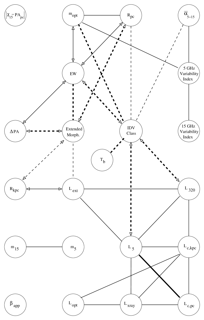
Figure 1: Diagram summarizing interrelations among source properties for the FS-PR sample (see Table 1 for symbol definitions). Solid lines indicate correlations found from Kendall’s tau tests. Dashed lines indicate significant population differences according to two-sample tests. Arrows denote anti-correlations, and lines in bold represent new correlations detected in this study.

4.2.1 Correlations with redshift

All of the luminosity variables in our dataset, with the exception of extended luminosity ($L_{ext}$), are correlated with redshift at better than $99.999\%$ confidence. This is expected, given the flux-limited nature of the FS-PR sample. None of the other (non-luminosity) variables are significantly correlated with redshift. We note that the BL Lacertae objects have significantly lower redshifts than the quasars in the sample (Table 5).

4.2.2 Correlations involving luminosity variables

The various luminosities of our sample objects are generally well-correlated with each other, but not with other source properties, as is indicated by their location in the lower right-hand corner of Figure 1. One major exception is IDV activity. Our two-sample tests indicate that sources that have not shown IDV tend to be more luminous at 320 MHz and 5 GHz. These trends may be due to beaming and selection effects in the sample (see §5.3).

Among luminosity-luminosity pairs, correlations involving the total 5 GHz luminosity ($L_{5}$) are the most prevalent. With the exception of $L_{5}$ versus the VLBI core luminosity ($L_{c,pc}$), all of the luminosity-luminosity correlations in Table 4 have been previously detected in other studies. The strong correlation between $L_{5}$ and $L_{c,pc}$ is merely a reflection of the highly core-dominated nature of the FS-PR sample.

4.2.3 Trends with polarization

The level of polarization at optical wavelengths has historically been an effective method of identifying highly beamed blazars whose jets are seen nearly end-on, since very few optically-selected quasars have $m_{opt}>3\%$ (Stockman et al., 1984). In Table 4 we confirm the previously known correlations with parsec-scale core dominance, 5 GHz radio variability amplitude, and emission line equivalent width that have helped establish $m_{opt}$ as a beaming indicator (see, e.g., Impey et al. 1991).

Xu et al. (1994) found that in the combined PR/Caltech-Jodrell samples, sources with low optical polarization levels $(<3\%)$ tend to have better jet alignments between parsec and kiloparsec scales than highly polarized sources. We find some indication of differences of these groups in the $m_{opt}$ - $\Delta PA$ plane (Fig. 2). There is a distinct grouping of sources in the lower left-hand portion of the plane which have both low optical polarization and small jet misalignments. The remainder of the sample shows a roughly linear trend of decreasing optical polarization with increasing jet misalignment.

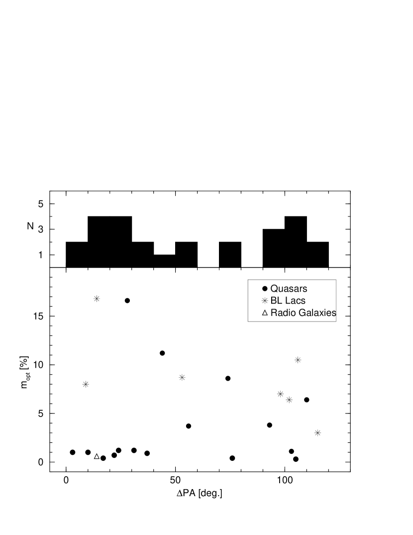
Figure 2: Top panel: histogram of pc/kpc-scale jet misalignment angle for the FS-PR sample. Bottom panel: jet misalignment angle plotted against optical polarization for various optical classes.

It is unclear whether the differences between the high and low-optically polarized objects in Fig. 2 can be entirely attributed to beaming and projection effects, which would tend to amplify any small intrinsic jet bends in sources seen nearly end-on. The current consensus is that blazars appear highly polarized since their optical synchrotron radiation is significantly boosted with respect to the underlying (thermal) continuum (the same process is responsible for lowering the observed emission line widths of highly beamed objects, e.g., Wills et al. 1992). If the optical synchrotron component is not highly polarized to begin with, however, the optical polarization will remain low, regardless of how beamed the source is. For example, Lister & Smith (2000) found evidence that many of the differences between HPQs and LPRQs are not due to differences in Doppler factor or jet orientation, but rather intrinsic differences in their jet magnetic field structures. It is possible that blazars go through temporary quiescent phases of low intrinsic polarization and flux variability, in which they appear as LPRQs (e.g., Fugmann, 1988). Long-term optical polarization monitoring studies of samples such as the FS-PR are needed to establish the properties of this duty cycle in blazars.

4.2.4 Properties of IDV sources

In an accompanying paper (Tingay et al., 2001), we discuss how the PR sources that have displayed type I and II IDV have substantially higher VSOP core brightness temperatures than those sources that have not displayed any IDV. Although it appears that the presence of a bright, compact core on VLBI scales is a necessary criterion for IDV (e.g., Heeschen et al. 1987; Quirrenbach et al. 1992), the phenomenon only occurs in $\mathrel{\hbox{\hbox to0.0pt{\hbox{\lower 4.0pt\hbox{$\sim$}}\hss}\hbox{$<$}}}2/3$ of all flat-spectrum radio sources (Quirrenbach et al., 1992; Kraus et al., 1999). Based on the IDV statistics of a large sample of AGNs, Quirrenbach et al. (1992) concluded that IDV was more prevalent in sources with $80\%$ or more of their total 5 GHz flux density contained in an unresolved VLBI core. We detect a similar trend in the FS-PR, with the $R_{pc}$ distribution of the type 0 (non-IDV) sources differing from that of the type II sources at the $99.918\%$ confidence level. The type 0 sources also have steeper radio spectral indices, in agreement with the findings of Quirrenbach et al. (1992).

We have also detected two additional trends that confirm the association of IDV with the blazar class. The IDV type I and II sources have higher optical polarization levels and narrower emission line equivalent widths than the type 0 objects. This suggests that the weak-lined BL Lac objects may be the best candidates for IDV; indeed, an optical study by Heidt & Wagner (1996) found IDV to be present in 28 of 34 BL Lacs selected from the 1 Jy catalog (Kühr et al., 1981).

The correlations with optical polarization and equivalent width suggest that the occurrence of IDV depends more on the Doppler factor of the source rather than any intrinsic property such as core size. As we will show in §5.3, the highest Doppler factor sources in a flux-limited sample such as the FS-PR are predicted to have low intrinsic (unbeamed) luminosities, according to the relativistic beaming model. Since the 320 MHz luminosity is generally accepted to be a good indicator of total jet power and intrinsic luminosity (Rawlings & Saunders 1991; Kaiser & Alexander 1997), this would imply that the type I and II IDV sources in the FS-PR should have lower $L_{320}$ values, which is in fact the case (Fig. 3).

Figure 3: Histograms of various properties for IDV type I & II (shaded) and non-IDV sources (un-shaded). Panel (A): optical polarization; (B): source frame equivalent width of widest permitted line; (C): luminosity at 320 MHz. (D): time-averaged spectral index between 5 and 14.5 GHz.

It is significant that we found no trends between IDV and beaming indicators on kiloparsec scales (i.e., $\Delta PA$, $R_{kpc}$, and morphological classification). This further implies that it is the Doppler factor of the innermost region of the jet that determines whether a source will display IDV.

4.2.5 Dependence of source properties on extended radio structure

Our correlation analysis has revealed that the arcsecond-scale radio morphology of core-dominated radio sources is closely connected with several other important source properties. In §3.1 we classified our sources as either compact, one-sided, two-sided, or halo based on their extended arcsecond-scale radio structure. Murphy (1988) analyzed the kiloparsec-scale properties of a large sample of core-dominated AGNs, and found that the two-sided sources tend to have lower core-dominance ratios ($R_{kpc}$) and stronger extended luminosities. We confirm these findings for the FS-PR, and additionally find that the two-sided sources have smaller parsec-scale core dominance, larger emission line equivalent widths, and smaller jet misalignments between parsec- and kiloparsec-scales (Fig. 4). Impey et al. (1991) found that the latter three properties are all highly influenced by source orientation, which implies that the jet axes of the two-sided sources are oriented farther away from the line of sight than the other sources in the FS-PR. It is conceivable that the two-sided sources might have intrinsically smaller core dominance and stronger extended power (irrespective of beaming), but we consider it unlikely that intrinsic differences could also conspire to mimic the trends with equivalent width and jet misalignment. Furthermore, there is strong evidence from unbeamed samples such as the 3C survey that the vast majority of powerful radio loud AGNs are intrinsically two-sided (Hintzen, Ulvestad & Owen, 1983). A simple explanation for the trends we see with sidedness is that for sources with jets seen nearly end-on, the emission from the hotspot on the far side of the one-sided sources is either beamed away from us, or is swamped by the highly beamed core in images of limited dynamic range.

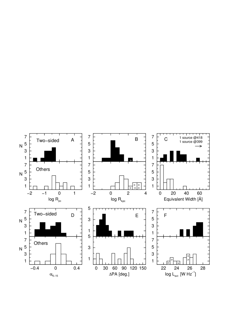
Figure 4: Histograms of various properties for sources with two-sided arcsecond-scale radio morphology (shaded) versus compact, one-sided and halo sources (un-shaded). Panel (A): parsec-scale core dominance ratio; (B): kiloparsec-scale core dominance ratio; (C): source frame equivalent width of widest permitted line; (D): time-averaged spectral index between 5 and 14.5 GHz; (E): pc/kpc-scale jet misalignment angle; (F): arcsecond-scale extended luminosity at 1.4 GHz.

4.2.6 Jet misalignment and bending

The difference in inner jet position angle between parsec and kiloparsec scales ($\Delta PA$) has been used in many studies as a general indicator of jet orientation. Since AGN jets are known to be intrinsically bent, those jets that are closer to the line of sight should have more exaggerated bends due to projection effects, and usually (but not necessarily) larger values of $\Delta PA$. Pearson & Readhead (1988) found unexpectedly that the distribution of $\Delta PA$ for the PR survey was bi-modal, with a clear division at approximately 45 degrees. Xu et al. (1994) found a similar result for the combined PR/Caltech-Jodrell samples. The reasons for this bi-modality are still unclear. Conway & Murphy (1993) have suggested that it could be due to selection effects associated with relativistic beaming and jet trajectories in the form of damped helices.

In the top panel of Figure 2 we show the distribution of $\Delta PA$ for the FS-PR sample, based on our improved parsec- and kiloparsec-scale jet position angle measurements described in §3.6. The bi-modality noticed by Pearson & Readhead (1988) is still present, with a division between aligned and misaligned sources occurring at roughly $60\arcdeg$. The vast majority of the aligned population ($\Delta PA<60\arcdeg$) have two-sided radio structure on arcsecond-scales (Fig. 4). This dependence of jet misalignment on lobe morphology strongly suggests that the highly misaligned sources have inner jets that are oriented closer to the line of sight. The observed trend of $\Delta PA$ with emission line equivalent width (also noticed by Appl et al. 1996 in a larger AGN sample) also supports this interpretation.

4.2.7 Parsec-scale core dominance

Numerous studies (e.g., Impey et al., 1991; Wills et al., 1992) have found that parsec-scale core dominance ($R_{pc}$) is likely a good beaming indicator, given that it is well-correlated with several other source properties that are affected by beaming. These include a strong anti-correlation with emission line equivalent width (Impey et al., 1991), and a positive correlation with optical polarization (Impey et al., 1991), both of which we confirm here (Table 4). In Figure 5 we show the distribution of parsec-scale core dominance for the various optical classes in the FS-PR sample. Our K-S tests reveal no statistically significant differences in these distributions.

Figure 5: Distribution of parsec-scale core dominance ($R_{pc}$) for various optical sub-classes of the FS-PR sample.

4.2.8 Kiloparsec-scale core dominance

In Figure 6 we show the distribution of kiloparsec-scale core dominance for the FS-PR. The measured values and limits span a remarkable range of at least four orders of magnitude, which reflects the wide variety of extended structure present in the sample (the parsec-scale core dominance spans only $\sim 2.5$ orders of magnitude in comparison). We confirm the finding of Morganti et al. (1995) that more highly core-dominated sources tend to have weaker extended luminosities.

The core dominance on kiloparsec scales is not correlated with any parsec-scale quantity for the FS-PR, such as emission line equivalent width, or optical polarization, as is the case for the parsec-scale core dominance. These correlations have been found, however, for non-core selected samples, e.g., Browne & Murphy (1987). It appears that VLA core dominance is not a useful indicator of inner jet orientation for samples selected on the basis of core flux density.

Figure 6: Distribution of kiloparsec-scale core dominance ($R_{kpc}$) for the FS-PR sample. Sources with lower limits are indicated by right arrows.

4.2.9 Apparent jet velocity

The maximum apparent jet velocity of a source is not necessarily a good indicator of relativistic beaming and jet orientation in core-selected samples, due to the non-linear dependence of apparent velocity ($\beta_{app}$) on viewing angle. Since the apparent velocity varies as $\beta\cos{\theta}/(1-\beta\cos{\theta})$, where $\beta$ is the true jet velocity in units of $c$ and $\theta$ is the viewing angle, highly beamed jets aligned within $1/\Gamma=\sqrt{1-\beta^{2}}$ radians to the line of sight can have rather low apparent velocities. We did not detect any correlations between apparent velocity and any other source property for the 20 FS-PR sources for which proper motion data are available. It appears that the full PR sample, which contains a wider range of jet viewing angles, may be better suited for exploring trends with apparent velocity.

4.2.10 Gamma-ray emission

The FS-PR sample contains seven AGNs that were detected in high-energy gamma-rays by the EGRET observatory. Our two-sample tests showed no significant differences in the properties of the EGRET versus non-EGRET objects. It is possible, however, that this null result may be due to the sample sizes (7 versus 25 objects), since the statistical reliability of Kolmogorov-Smirnov tests is greatly decreased for such small samples (Press et al., 1992).

5 Discussion

5.1 Cluster analysis

Our network diagram (Fig. 1) graphically displays the relationships between the various properties of the FS-PR sources. In order to investigate possible groupings in this diagram, we have applied a cluster analysis to our data (e.g., Nair, 1997). This method searches for natural groupings among variables that are most correlated. The most common (“single-link”) method involves taking a symmetric matrix of correlation coefficients $r_{ij}$ and finding the two variables $a$ and $b$ that are the best correlated. These two variables are replaced by a new “cluster” variable $c$, for which $r_{ci}=\max[r_{ai},r_{bi}]$. The process is repeated until there is only one cluster variable remaining. The results are usually presented in the form of a tree diagram, in which the clusters are represented by branches.

A few modifications to the standard cluster method were needed to apply it to our data. Since our computed correlation coefficients for censored variables have a different form of variance than the uncensored ones (Akritas & Siebert, 1996), they cannot be directly inter-compared. Also, the fact that many of our variables have a mutual dependence on redshift will artificially skew the shape of the cluster tree diagram. We have therefore taken the following steps in order to arrive at a more accurate representation of the true cluster tree. First, we have used the statistical significance levels in place of the correlation coefficients to compare the variables. For the two nominal variables (IDV and extended morphology class), we have used the two-sample test significance levels. Second, we have used the significance levels with redshift partialed out for all of the luminosity variables. Finally, we have replaced the significance level for the rejected correlations listed in Table 4 with a value that excludes the outlier point.

We show the resulting tree diagram in Figure 7. The vertical connections indicate a close connection between variables and groups of variables. The horizontal axis is roughly proportional to correlation strength, with the vertical bars located furthest to the right representing the strongest correlations. The luminosity variables form a distinct grouping since they are poorly correlated with the remaining variables. The apparent jet velocity and fractional polarization levels at 5 & 15 GHz also form a distinct group that is largely independent of other source properties.

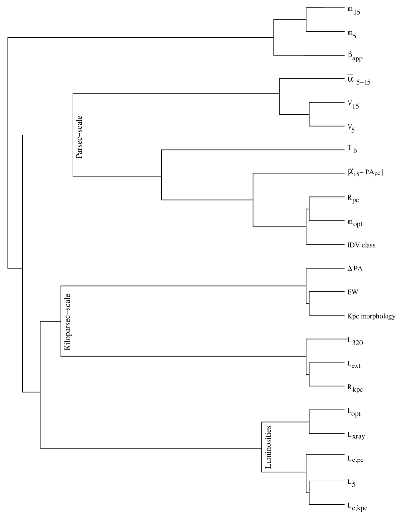
Figure 7: Cluster diagram for source properties of the FS-PR sample. For symbol definitions, see Table 1.

Among the remaining variables, those associated with the parsec-scale core form a distinct grouping (labeled “parsec scale” in Fig. 7). The emission line equivalent width, kiloparsec-scale morphology, and jet misalignment angle form a separate grouping. The exclusion of the equivalent width from the parsec-scale grouping is somewhat unexpected, given that the broad line region in quasars is thought to be less than a parsec in extent (Capriotti, Foltz & Peterson, 1982). This may imply that the kiloparsec-scale properties of jets such as bending are influenced by the intrinsic line strength, and in turn the density of the broad line gas.

5.2 Emission line strength and the BL Lacertae class

Early VLBI studies of AGN samples with complete optical spectra (e.g. Impey et al. 1991) showed that emission line strength was correlated with core dominance on parsec-scales, and led to a model in which the optical continuum in highly beamed sources is dominated by synchrotron emission from the jet (Wills et al., 1992). Since the emission from the broad line region is unbeamed, the ratio of line to continuum flux (as well as emission line equivalent width) should steadily decrease with viewing angle to the source. Also, the overall optical polarization should increase, as the polarized synchrotron component begins to dominate. All of these predictions are borne out in the FS-PR, as evidenced by the mutual correlations between equivalent width, $\Delta PA$ and extended morphology.

These correlations have potentially important implications for the BL Lacertae class of AGN, which by definition have low emission line equivalent widths. Several studies have shown that these objects have intrinsically different properties than their broad-lined counterparts, the high optically-polarized quasars (HPQs). These include differences in their parsec-scale magnetic fields (Cawthorne et al., 1993), X-ray spectral shapes (Worrall & Wilkes, 1990), and extended radio power (Padovani, 1992). It has been suggested that the parent population of the BL Lacs are FR-I type radio galaxies, while the radio quasars belong to the more powerful FR-II population (see Urry & Padovani 1995 and references therein).

The nine BL Lacs in the FS-PR rank in the top $30\%$ of the sample in terms of optical polarization, $\Delta PA$ values, 5 GHz variability amplitude, and parsec-scale core dominance. This implies that they are indeed highly beamed objects. There remains some debate over whether BL Lacs are in fact more beamed (i.e., have higher Doppler factors) than high-optically polarized quasars. The FS-PR sample is not ideally suited to fully investigate this issue, since it contains only nine BL Lacs and nine confirmed HPQs. Nevertheless, we have performed several K-S tests on our data, and find that although the BL Lacs do tend to have lower than average redshifts, there are otherwise no significant differences in the $\Delta PA$, optical polarization, variability amplitude, and core dominance distributions of the two classes. Therefore, despite strong indications that the observed equivalent width in core-dominated radio sources is highly dependent on beaming, there is insufficient evidence in the FS-PR to support a claim that BL Lacs are more highly beamed than HPQs. This hypothesis should not be ruled out, however, until a similar analysis can be conducted on a much larger sample such as the Caltech-Jodrell Flat-spectrum survey (CJ-F; Taylor et al. 1996).

5.3 Relativistic beaming simulations

In the previous discussion we have made reference to general predictions of the relativistic beaming model, and how it can account for many of the correlations seen in the FS-PR sample. In this section we describe in more detail the predicted properties of sources in core-selected, flux-limited samples, based on Monte Carlo beaming simulations.

Simulations of relativistic beaming by Vermeulen & Cohen (1994) and others have shown that core-selected samples should be dominated by objects with jets pointing nearly directly at us. This would suggest that the FS-PR should contain a narrow range of highly beamed, high-Doppler factor sources. It is essential to consider, however, the additional effects of the luminosity function (LF) and redshift distribution of the FS-PR parent population. It is very likely that some low-Doppler factor sources that happen to be intrinsically very luminous or relatively nearby may have also been included in the FS-PR sample. This would explain the presence of the two radio galaxies (3C 84 and 2021+614), which are generally considered to be a weakly beamed class of AGN (Urry & Padovani, 1995). It would also account for the large range of kiloparsec-scale core dominance found within the sample. The effects of adding a LF and redshift distribution to beaming models have been investigated by Lister & Marscher (1997). They found that samples such as the FS-PR should in fact contain a wide range of Doppler factors. In this section we use the model of Lister & Marscher (1997) to show how many of the correlations in the FS-PR are likely a result of a mutual dependence of source properties on Doppler factor.

Lister & Marscher (1997) used their Monte Carlo model to successfully fit various properties of the Caltech-Jodrell Flat-spectrum sample (CJF; Taylor et al. 1996), of which the FS-PR is a sub-set. Their best-fit parent population contains a power law jet Lorentz factor distribution of the form $N(\Gamma)\propto\Gamma^{-1.25}$ with $1.001252<\Gamma<30$. The jets are randomly oriented in space, and distributed with a constant co-moving space density out to $z=4$. The jet luminosity function mirrors that of the FR-II radio galaxies, which was derived by Urry & Padovani (1995), and incorporates pure exponential luminosity evolution. The jets are assumed to be two-sided, and have luminosities that are Doppler boosted by a factor of $\delta^{2}$. In a typical model run, parent objects are continuously created until 293 sources with flux density exceeding 0.35 Jy (the CJF sample size and cutoff) are obtained. Further details of the model can be found in Lister & Marscher (1997).

In Figures 8, 9, and 10 we plot the results of a single Monte Carlo simulation with the above parameters that illustrates several of the strong biases that are present in flux-limited samples. The small circles represent the 293 simulated CJF sources, and larger circles indicated sources brighter than 1.3 Jy (the FS-PR cutoff). Figure 8 plots the intrinsic luminosity of the jet (removing the Doppler boosting effect) against Doppler factor. The upper envelope to the distribution indicates that extremely powerful sources that are also highly beamed are exceedingly rare, and that weakly beamed sources generally need to be more intrinsically luminous to be included in flux-limited samples. This trend provides a natural explanation for the observation that IDV type 0 sources generally have stronger 320 MHz and 5 GHz luminosities than the IDV type I and II sources in the FS-PR, since the non-IDVs are expected to be less relativistically boosted (see §4.2.4).

Figure 8: Plot of intrinsic (unbeamed) 5 GHz jet luminosity vs. Doppler factor for a simulated Caltech-Jodrell Flat-spectrum sample (small circles) and a simulated FS-PR sample (large circles).

In Figure 9 we plot two quantities against the jet Lorentz factor: apparent velocity (upper panel), and viewing angle (lower panel). The solid lines on these panels indicate the positions of sources seen at the viewing angle that maximizes the apparent velocity ($\theta=\arcsin{[1/\Gamma]}$). As pointed out by Lister & Marscher (1997), there is a substantial spread around this angle (lower panel), with most sources seen at significantly smaller angles to the line of sight. Nevertheless, the fairly good correlation in the upper panel suggests that apparent velocity can be used as a statistical indicator of the Lorentz factor. We note, however, that our simulations assume the observed pattern speed reflects the true speed of the jet, which may not be the case for all sources (Vermeulen & Cohen, 1994).

Figure 9: Upper panel: Plot of apparent velocity vs. Lorentz factor for a simulated Caltech-Jodrell Flat-spectrum sample (small circles) and a simulated FS-PR sample (large circles). Bottom panel: Plot of viewing angle vs. Lorentz factor. The solid lines in both panels indicate the position of sources seen at a viewing angle that maximizes the apparent velocity.

The apparent velocity of a jet by itself is not a good indicator of viewing angle (lower panel of Fig. 10), due to the preponderance of jets seen within the $1/\Gamma$ viewing cone. At best it can be used to set an upper limit on the viewing angle, through the well known formula $\theta\leq\arccos{[(\beta_{app}^{2}-1)/(\beta_{app}^{2}+1)]}$. The lack of a good correlation between apparent velocity and viewing angle may explain why the former quantity is not correlated with other source properties in the FS-PR. Alternatively, the measured apparent speeds could simply be pattern speeds that do not reflect the true jet Lorentz factor. If this is the case, the best statistical approach would be to use long-term VLBI monitoring to determine a maximum observed velocity for each source in a large sample.

The upper panel of Fig. 10 shows that we can expect an extremely good correlation between viewing angle and Doppler factor in a small flux-limited sample such as the FS-PR, provided the parent population has an upper Lorentz factor limit. This trend is likely the source of correlations between orientation-dependent properties (e.g., jet misalignment angle and arcsecond-scale morphology) and Doppler boosting-dependent properties (e.g., core dominance and emission line equivalent width).

Figure 10: Upper panel: Plot of jet Doppler factor vs. viewing angle for a simulated Caltech-Jodrell Flat-spectrum sample (small circles) and a simulated FS-PR sample (large circles). Bottom panel: Plot of apparent velocity vs. viewing angle. The solid lines in both panels indicate the position of a source with Lorentz factor 30, and the dashed lines indicate a source with Lorentz factor 5.

5.4 The identification of highly beamed radio sources

The Doppler factors of extragalactic jets are notoriously difficult to measure accurately, due to a lack of good indicators of true jet velocity and orientation. Although some highly beamed sources can be recognized on the basis of blazar properties (i.e., high variability and optical polarization), other beamed sources may have intrinsically low variability and/or polarization. Our analysis of the FS-PR sample suggests a set of criteria that can be used to identify the AGNs with the highest Doppler factors in core-selected samples. In general, the most highly beamed sources will tend to have a) flat radio spectra, b) a type I or II IDV classification; c) one-sided, halo-like, or no extended structure on kiloparsec scales; d) a relatively large ($\mathrel{\hbox{\hbox to0.0pt{\hbox{\lower 4.0pt\hbox{$\sim$}}\hss}\hbox{$>$}}}60\arcdeg$) misalignment between their jet directions on parsec and kiloparsec scales; e) optical polarization that has exceeded $\sim 3\%$ on at least one occasion; f) relatively high core dominance on parsec ($R_{pc}\mathrel{\hbox{\hbox to0.0pt{\hbox{\lower 4.0pt\hbox{$\sim$}}\hss}\hbox{$>$}}}0.3$) and kiloparsec ($R_{kpc}\mathrel{\hbox{\hbox to0.0pt{\hbox{\lower 4.0pt\hbox{$\sim$}}\hss}\hbox{$>$}}}10$) scales; g) an equivalent width of the largest permitted emission line smaller than $\sim 15$ Å (source frame); and h) a 5 GHz source frame core brightness temperature exceeding $10^{11}\rm K$.

After taking into account the missing data on some of our sources, there are three HPQs (0133+476, 0804+499, and 1739+522) and six BL Lacs (0454+844, 0954+658, MK 501, 1749+701, 1803+784, and BL Lacertae) in the FS-PR that are consistent with the above criteria. We suggest that these sources have significantly higher Doppler factors than the other sources in the FS-PR, and should be considered as prime targets for high-frequency space-VLBI and IDV monitoring observations. We predict that two of these objects (0454+844 and 1739+522) will eventually be found to display type I or II IDV, based on their other properties.

6 Conclusions and suggestions for future work

We have obtained data using the facilities of the VSOP mission and from the literature on a flat-spectrum, core-selected subsample of the Pearson-Readhead AGN survey (the FS-PR sample) in order to investigate the effects of relativistic beaming in compact radio sources. The main results of our multi-dimensional correlation analysis on these data are as follows:

(i) The properties of sources that have displayed type I or II IDV are significantly different than those that have shown no IDV activity. They have flatter spectral indices, higher core dominance on parsec scales, higher optical polarizations and smaller emission line widths. They also have lower 320 MHz and 5 GHz luminosities and weaker kiloparsec-scale core components. These findings are all consistent with Monte Carlo beaming simulations which predict that higher Doppler factor sources in flux-limited generally have weaker intrinsic luminosities.

(ii) The observed luminosity properties of the FS-PR are generally well-correlated with each other, but not with other properties of the sample. The only exception is the trend with IDV described above.

(iii) The high-optically polarized sources in the FS-PR show a trend of increased parsec-to-kiloparsec jet misalignment ($\Delta PA$) with decreasing optical polarization. However, the lowest optically polarized sources ($m_{opt}<3\%$) generally have small jet misalignments, which may suggest that they have intrinsically different jet properties.

(iv) We find that sources with two-sided radio morphology on kiloparsec-scales have significantly different properties than other sources in the FS-PR. They tend to be less core dominated on parsec- and kiloparsec scales, and have stronger extended luminosities and larger emission line widths. Their jets are also less misaligned between parsec- and kiloparsec scales, which suggests that they are oriented at angles farther away from the line of sight.

(v) We have used high-resolution VLBI images to confirm the bi-modality of the $\Delta PA$ distribution for the PR sample (Pearson & Readhead, 1988), with a division occurring $\Delta PA\simeq 60\arcdeg$. The aligned sources tend to have broader emission line equivalent widths than the misaligned population.

(vi) We did not find any correlations between maximum apparent jet velocity and other source properties. This may be due to the predicted weak dependence of $\beta_{app}$ on viewing angle for core-selected samples, or the fact that the measured speeds may not reflect the true bulk speeds of the emitting material in the jet.

(vii) The nine BL Lacertae objects in the FS-PR rank among the top $30\%$ of the sample in terms of their optical polarization, $\Delta PA$ values, 5 GHz variability amplitude, and parsec-scale core dominance, which suggests that they are highly beamed objects. We found no significant differences in their properties as compared to the high-polarization quasars, other than the fact that they have smaller redshifts.

(viii) Our correlation analysis and Monte Carlo beaming simulations have shown that the properties of the FS-PR sample are remarkably consistent with the predictions of the relativistic beaming model. The majority of the observed correlations are likely due to a mutual dependence of source properties on the jet Doppler factor and viewing angle, and do not necessarily reflect intrinsic relations among jet properties.

Our work has demonstrated the merits of obtaining a wide variety of data on a relatively small sample, and suggests several further observations that can improve our understanding of the beaming phenomenon in AGNs. These include optical variability monitoring of the PR survey to further investigate the connection between optical and radio properties, and more uniform monitoring of the sample for IDV activity in the radio. It will also be important to measure apparent velocities for the remaining sources in the sample, and to obtain high-dynamic range VLA and MERLIN maps down to a uniform luminosity level. The latter can be used to trace out bending in the jets as they propagate from parsec- to kiloparsec scales, and examine how this phenomenon is influenced by other source properties. With regular monitoring the optical polarization of the sample at regular intervals, it should be possible to establish a duty cycle of optical polarization in blazars, and to better understand the inherent differences in high- and low-optically polarized AGNs.

Table 1: Measured and Derived Quantities for the Pearson-Readhead AGN Sample

Symbol	Property	Units	Reference
General Properties
$\cdots$	EGRET gamma-ray detection/non-detection	$\cdots$	Hartman et al. 1999
$\cdots$	Optical classification (RG, LPRQ, HPQ, BL Lac)	$\cdots$	Various
$\cdots$	Kiloparsec-scale extended morphology	$\cdots$	Various
$z$	Redshift	$\cdots$	Lawrence et al. 1996
$EW$	Equivalent width of widest permitted line (source frame)	Å	Lawrence et al. 1996
$\bar{\alpha}_{5-15}$	Time-averaged spectral index between 4.8 and 14.5 GHz	$\cdots$	Aller et al. 1992
Variability Properties
$V_{5}$	Variability amplitude at 5 GHz	$\cdots$	Aller et al. 1992
$V_{15}$	Variability amplitude at 14.5 GHz	$\cdots$	Aller et al. 1992
$\cdots$	IDV classification	$\cdots$	Various
Luminosity Properties
$L_{320}$	Total luminosity at 320 MHz	$\rm W\;Hz^{-1}$	Impey et al. 1991
$L_{5}$	Total luminosity at 5 GHz	$\rm W\;Hz^{-1}$	UMRAO database
$L_{opt}$	Optical V band luminosity	$\rm W\;Hz^{-1}$	NED
$L_{xray}$	X-ray luminosity at 1 keV	$\rm W\;Hz^{-1}$	Various
$L_{c,pc}$	Parsec-scale core luminosity at 5 GHz	$\rm W\;Hz^{-1}$	This paper
$L_{c,kpc}$	Kiloparsec-scale core luminosity at 1.4 GHz	$\rm W\;Hz^{-1}$	Various
$L_{ext}$	Total arcsecond-scale extended luminosity at 1.4 GHz	$\rm W\;Hz^{-1}$	Various
Jet Properties
$T_{b}$	Brightness temperature of VLBI core component	K	Tingay et al. (2001)
$R_{pc}$	Ratio of parsec-scale core to remaining flux density	$\cdots$	This paper
$R_{kpc}$	Ratio of kiloparsec-scale core to remaining flux density	$\cdots$	Various
$\beta_{app}$	Fastest measured apparent speed of jet component	$\cdots$	Various
$\Delta{PA}$	Difference in position angle between pc-and kpc-scale jet	Deg.	Various
Polarization Properties
$m_{opt}$	Optical V band linear polarization	$\%$	Impey et al. 1991
$m_{5}$	Mean linear polarization at 4.8 GHz	$\%$	Aller et al. 1992
$m_{15}$	Mean linear polarization at 14.5 GHz	$\%$	Aller et al. 1992
$|\chi_{15}-PA_{pc}|$	Offset of integrated 14.5 GHz $\chi$ w.r.t. pc-scale jet PA	Deg.	Aller et al. 1992

Note. — Data on properties marked “Various” were gathered from multiple sources (see §3).

Table 2: General Properties of Pearson-Readhead Sources

IAU	Other	Opt.		IDV					log			log
Name	Name	Type	Morph.	Class	z	EW	$L_{c,pc}$	$L_{5}$	$R_{pc}$	$L_{c,kpc}$	$L_{ext}$	$R_{kpc}$	Ref.	$L_{xray}$	Ref.
[1]	[2]	[3]	[4]	[5]	[6]	[7]	[8]	[9]	[10]	[11]	[12]	[13]	[14]	[15]	[16]
FS-PR sample objects
0016+731	$\cdots$	Q	2	I	1.781	17.0	26.99	27.93	–0.89	27.90	$<$25.57	$>$2.33	1	20.97	8
0133+476	OC 457	HPQ	C	II	0.859	10.4	27.46	27.53	0.75	27.34	$<$24.26	$>$3.08	1	20.96	8
0212+735	$\cdots$	HPQ	C	0	2.367	15.0	28.25	28.78	–0.37	28.56	$<$25.59	$>$2.97	1	22.01	8
0316+413	3C 84	RG	2	0	0.017	417.5	24.07	25.22	–1.12	25.05	24.58	0.47	2	18.00	9
0454+844	$\cdots$	BL	C	$\cdots$	0.112	$<$1.0	$\cdots$	25.30	$\cdots$	25.09	$<$22.71	$>$2.38	3	18.01	10
0723+679	3C 179	LPRQ	2	$\cdots$	0.844	39.2	$\cdots$	$\cdots$	$\cdots$	26.81	27.76	–0.95	4	$\cdots$	$\cdots$
0804+499	OJ 508	HPQ	1	II	1.432	13.0	$\cdots$	27.90	$\cdots$	27.53	25.75	1.78	3	21.23	8
0814+425	OJ 425	BL	1	II	0.245	1.0	25.83	26.19	–0.11	26.38	25.07	1.30	3	18.95	10
0836+710	4C 71.07	Q	2	0	2.180	17.6	27.88	28.51	–0.52	28.67	27.51	1.16	3	22.83	8
0850+581	4C 58.17	LPRQ	2	$\cdots$	1.322	25.9	$\cdots$	27.69	$\cdots$	27.48	26.73	0.75	4	20.79	11
0859+470	4C 47.29	Q	2	0	1.462	30.0	27.39	27.95	–0.42	27.96	27.55	0.40	3	20.70	11
0906+430	3C 216	HPQ	2	I	0.670	3.1	26.74	27.32	–0.45	26.92	27.22	–0.30	5	20.23	8
0923+392	4C 39.25	LPRQ	2	0	0.699	58.3	26.52	28.11	–1.58	27.52	27.09	0.43	3	20.99	8
0945+408	4C 40.24	LPRQ	1	I	1.252	15.9	$\cdots$	27.78	$\cdots$	27.69	26.86	0.83	3	20.93	8
0954+556	4C 55.17	HPQ	2	$\cdots$	0.900	7.1	$\cdots$	$\cdots$	$\cdots$	27.72	27.11	0.61	3	20.53	8
0954+658	$\cdots$	BL	1	II	0.367	1.9	$\cdots$	26.48	$\cdots$	26.23	25.17	1.06	6	19.84	10
1624+416	4C 41.32	Q	1	0	2.550	13.6	27.42	28.39	–0.92	28.45	$<$25.85	$>$2.60	3	$\cdots$	$\cdots$
1633+382	4C 38.41	HPQ	2	0	1.807	38.1	27.58	28.36	–0.70	28.27	26.79	1.47	3	21.88	8
1637+574	OS 562	Q	H	$\cdots$	0.749	17.3	26.53	27.01	–0.30	27.22	26.52	0.70	3	20.62	11
1641+399	3C 345	HPQ	2	0	0.595	34.9	26.86	27.86	–0.96	27.88	27.11	0.76	3	20.69	8
1642+690	4C 69.21	HPQ	2	II	0.751	26.0	26.75	27.22	–0.29	27.15	26.87	0.29	3	$\cdots$	$\cdots$
1652+398	MK 501	BL	H	I	0.033	0.8	24.09	24.66	–0.44	24.57	23.27	1.29	5	19.37	10
1739+522	4C 51.37	HPQ	1	$\cdots$	1.381	8.1	27.93	28.07	0.43	28.02	26.27	1.75	4	21.20	12
1749+701	$\cdots$	BL	1	II	0.770	0.2	26.60	26.98	–0.15	$\cdots$	$\cdots$	$\cdots$	14	20.55	10
1803+784	$\cdots$	BL	1	II	0.680	2.9	27.20	27.38	0.29	27.26	26.08	1.18	3	20.61	10
1807+698	3C 371	BL	2	I	0.050	6.0	24.39	25.01	–0.50	24.89	24.81	0.07	5	18.32	10
1823+568	4C 56.27	BL	1	I	0.663	1.1	26.94	27.23	0.02	26.88	26.88	0.00	3	20.84	10
1928+738	4C 73.18	LPRQ	2	I	0.302	398.9	25.98	26.92	–0.89	26.83	25.84	0.99	3	20.52	8
1954+513	OV 591	Q	2	$\cdots$	1.223	18.3	27.08	27.79	–0.61	27.72	27.61	0.11	7	$\cdots$	$\cdots$
2021+614	OW 637	RG	C	0	0.228	35.4	25.01	26.56	–1.54	26.45	$<$23.19	$>$3.27	1	$\cdots$	$\cdots$
2200+420	BL Lac	BL	H	I	0.069	6.8	25.27	25.72	–0.27	25.57	23.70	1.87	5	19.04	10
2351+456	4C 45.51	Q	2	0	1.986	25.3	$\cdots$	28.16	$\cdots$	$\cdots$	$\cdots$	$\cdots$	13	$\cdots$	$\cdots$
VSOP-PR sample objects
0153+744	$\cdots$	Q	C	I	2.338	14.6	27.71	28.96	–1.23	28.41	$<$25.53	$>$2.88	1	22.36	8
0711+356	OI 318	Q	2	II	1.620	19.1	26.72	28.20	–1.47	28.02	25.79	2.23	3	20.77	$\cdots$
1828+487	3C 380	LPRQ	2	$\cdots$	0.692	36.1	26.79	27.91	–1.09	27.73	28.15	–0.42	3	21.08	9

Note. — All quantities are calculated assuming $h=0.65$, $q_{o}=0.1$, and $\Lambda=0$. Luminosities are given in $\rm W\;Hz^{-1}$. Columns are as follows: (1) IAU source name; (2) Alternate name; (3) Optical classification (see §3.1); (4) Kiloparsec-scale radio morphology, where C = compact, 1 = one-sided, 2 = two-sided, and H = halo; (5) IDV classification (see §3.2); (6) Redshift; (7) Source frame equivalent width of widest permitted line [Å]; (8) Luminosity of parsec-scale core component at 5 GHz; (9) Total (single-dish) luminosity of source at 5 GHz; (10) Ratio of parsec-scale core flux density to remaining (non-core) flux density at 5 GHz in source rest frame; (11) Luminosity of kiloparsec-scale core component at 1.4 GHz; (12) Luminosity of kiloparsec-scale extended structure at 1.4 GHz; (13) Ratio of kiloparsec-scale core to extended flux density at 1.4 GHz, in source rest frame; (14) Reference for columns 4, 11 and 12; (15) X-ray luminosity at 0.1 keV; (16) Reference for X-ray data.

References. — (1) Xu et al. 1995; (2) Pedlar et al. 1990; (3) Murphy, Browne, & Perley 1993; (4) Reid et al. 1995; (5) Antonucci & Ulvestad 1985; (6) Cassaro et al. 1999; (7) Browne & Perley 1986; (8) Sambruna 1997; (9) Hardcastle & Worrall 1999; (10) Urry et al. 1996; (11) Perlman et al. 1998; (12) Comastri et al. 1997; (13) Neff, Roberts, & Hutchings 1995; (14) O’Dea, Barvainis, & Challis 1988.

Table 3: Jet Properties of Pearson-Readhead Sources

Source	$\beta_{app}$		$PA_{pc}$	$PA_{kpc}$	$\Delta{PA}$
Name	$(v/c)$	Ref.	(deg)	(deg)	(deg)	Ref.
[1]	[2]	[3]	[4]	[5]	[6]	[7]
FS-PR sample objects
0016+731	17.3	2	132	169	37	22, 25
0133+476	$\cdots$	$\cdots$	330	$\cdots$	$\cdots$	22, $\cdots$
0212+735	8.6	4	121	$\cdots$	$\cdots$	22, $\cdots$
0316+413	0.08	5	176	162	14	22, 26
0454+844	1.1	6	177	$\cdots$	$\cdots$	22, $\cdots$
0723+679	8.6	8	256	266	10	22, 38
0804+499	$\cdots$	$\cdots$	127	201	74	22, 27
0814+425	$\cdots$	$\cdots$	103	50	53	22, 27
0836+710	21.7	9	201	198	3	22, 29
0850+581	7.6	10	227	151	76	22, 30
0859+470	$\cdots$	$\cdots$	357	335	22	22, 28
0906+430	5.3	11	151	244	93	22, 31
0923+392	2.3	12	93	76	17	21, 32
0945+408	$\cdots$	$\cdots$	137	32	105	22, 28
0954+556	$\cdots$	$\cdots$	191	301	110	23, 28
0954+658	12.2	13	326	224	102	22, 33
1624+416	$\cdots$	$\cdots$	261	351	90	1, 34
1633+382	15.9	14	279	176	103	21, 27
1637+574	$\cdots$	$\cdots$	200	$\cdots$	$\cdots$	22, $\cdots$
1641+399	29.3	15	284	328	44	21, 35
1642+690	14.0	16	158	186	28	22, 34
1652+398	5.6	17	160	45	115	22, 36
1739+522	$\cdots$	$\cdots$	204	260	56	22, 28
1749+701	10.9	2	275	21	106	22, 25
1803+784	3.2	13	291	193	98	22, 27
1807+698	$\cdots$	$\cdots$	252	261	9	22, 36
1823+568	21.2	14	196	182	14	22, 34
1928+738	11.5	4	166	190	24	21, 27
1954+513	$\cdots$	$\cdots$	307	338	31	22, 24
2021+614	0.19	19	205	$\cdots$	$\cdots$	19, $\cdots$
2200+420	13.0	20	209	$\cdots$	$\cdots$	22, $\cdots$
2351+456	$\cdots$	$\cdots$	321	348	27	22, 39
VSOP-PR sample objects
0153+744	3.8	3	68	$\cdots$	$\cdots$	22, $\cdots$
0711+356	$<0.81$	7	329	294	35	22, 27
1828+487	10.6	18	311	311	0	22, 37

Note. — Columns are as follows: (1) IAU source name; (2) Maximum component speed in units of $c$, assuming $h=0.65$ and $q_{o}=0.1$; (3) Reference for apparent speed; (4) Parsec-scale jet position angle; (5) Kiloparsec-scale jet position angle. (6) Difference in parsec- and kiloparsec-scale jet position angles; (7) References for images used in columns 4 and 5, respectively.

References. — (1) Lister et al. 2001; (2) Schalinski et al. 1992; (3) Hummel et al. 1997; (4) Witzel et al. 1988; (5) Dhawan, Kellerman, & Romney 1998; (6) Gabuzda et al. 1994; (7) Conway et al. 1994; (8) Porcas 1987; (9) Marchenko-Jorstad et al. 2000; (10) Barthel et al. 1986; (11) Paragi et al. 2000; (12) Fey, Eubanks, & Kingham 1997; (13) Gabuzda & Cawthorne 1996; (14) S. G. Jorstad, private communication; (15) Ros, Zensus, & Lobanov 2000; (16) Pearson et al. 1986; (17) Giovannini et al. 2000; (18) Polatidis & Wilkinson 1998; (19) Tschager et al. 1999; (20) Denn, Mutel, & Marscher 2000; (21) Lister & Smith 2000; (22) Lister et al., in preparation; (23) A. P. Marscher, private communication; (24) Kollgaard, Wardle, & Roberts 1990; (25) Xu et al. 1995; (26) Pedlar et al. 1990; (27) Murphy, Browne, & Perley 1993; (28) Reid et al. 1995; (29) Hummel et al. 1992; (30) Shone, Porcas, & Zensus 1985; (31) Taylor, Ge, & O’Dea 1995; (32) Marscher et al. 1991; (33) Stanghellini et al. 1997; (34) O’Dea, Barvainis, & Challis 1988; (35) Kollgaard, Wardle, & Roberts 1989; (36) Cassaro et al. 1999; (37) Lüdke et al. 1998; (38) Akujor 1992; (39) Neff, Roberts, & Hutchings 1995.

Table 4: Correlations Among Observed Properties of the FS-PR Sample

Property	Property	N	$\tau$	P	$\tau_{z}$	$P_{z}$	Notes
(1)	(2)	(3)	(4)	(5)	(6)	(7)	(8)
$L_{ext}$	$R_{kpc}$	30	–0.56	$9.7\times 10^{-4}$	–0.60	$4.9\times 10^{-12}$	Expected
$R_{pc}$	$EW$	24	–0.49	$8.1\times 10^{-2}$	–0.50	$1.8\times 10^{-7}$	Impey et al. (1991)
$L_{5}$	$L_{c,kpc}$	28	0.91	$1.1\times 10^{-9}$	0.77	$7.6\times 10^{-7}$	Akritas & Siebert (1996)
$V_{15}$	$V_{5}$	31	0.62	$9.6\times 10^{-5}$	0.63	$7.2\times 10^{-5}$	Aller et al. (1992)
$L_{ext}$	$L_{320}$	28	0.48	$2.4\times 10^{-2}$	0.49	$9.2\times 10^{-4}$	Expected
$m_{opt}$	$EW$	30	–0.42	$1.2\times 10^{-1}$	–0.40	$2.1\times 10^{-2}$	Impey et al. (1991)
$L_{5}$	$L_{xray}$	25	0.79	$3.6\times 10^{-6}$	0.52	$2.6\times 10^{-2}$	Browne & Murphy (1987)
$L_{opt}$	$L_{xray}$	26	0.67	$1.4\times 10^{-4}$	0.52	$2.6\times 10^{-2}$	Fabbiano et al. (1984)
$R_{pc}$	$m_{opt}$	23	0.50	$8.2\times 10^{-2}$	0.52	$4.5\times 10^{-2}$	Impey et al. (1991)
$\Delta{PA}$	$EW$	26	–0.39	$5.5\times 10^{-1}$	–0.40	$2.0\times 10^{-1}$	Appl et al. (1996)
$L_{5}$	$L_{320}$	27	0.69	$5.1\times 10^{-5}$	0.42	$2.2\times 10^{-1}$	Zirbel & Baum (1995)
$L_{5}$	$L_{c,pc}$	24	0.75	$2.5\times 10^{-5}$	0.41	$4.8\times 10^{-1}$	$\cdots$
$L_{c,pc}$	$L_{c,kpc}$	23	0.76	$4.6\times 10^{-5}$	0.42	$4.9\times 10^{-1}$	Expected
$m_{15}$	$m_{5}$	31	0.34	$7.2\times 10^{-1}$	0.34	$7.1\times 10^{-1}$	Aller et al. (1992)
$L_{ext}$	$L_{5}$	28	0.33	1.1	0.25	$9.3\times 10^{-1}$	Expected
$L_{c,kpc}$	$L_{xray}$	25	0.71	$2.5\times 10^{-5}$	0.41	1.2	Browne & Murphy (1987)
$L_{c,pc}$	$L_{xray}$	20	0.72	$1.0\times 10^{-3}$	0.39	1.6	Bloom et al. (1999)
$L_{opt}$	$L_{c,kpc}$	30	0.60	$3.2\times 10^{-4}$	0.31	1.7	Feretti et al. (1984)
$V_{5}$	$\bar{\alpha}_{5/15}$	31	0.30	1.6	0.30	1.7	Aller et al. (1992)
$L_{c,kpc}$	$L_{320}$	28	0.63	$2.3\times 10^{-4}$	0.31	1.9	Fabbiano et al. (1984)
$m_{opt}$	$V_{5}$	29	0.33	1.3	0.31	2.0	Valtaoja et al. (1992)
Correlations likely due to redshift bias
$L_{opt}$	$\beta_{app}$	20	0.38	2.0	0.27	4.4	$\cdots$
$L_{opt}$	$L_{c,pc}$	24	0.58	$8.4\times 10^{-3}$	0.28	6.0	$\cdots$
$L_{opt}$	$L_{5}$	30	0.54	$2.4\times 10^{-3}$	0.20	13	$\cdots$
$L_{c,pc}$	$L_{320}$	22	0.56	$2.8\times 10^{-2}$	0.19	22	$\cdots$
$L_{320}$	$L_{xray}$	23	0.48	$1.4\times 10^{-1}$	0.07	65	$\cdots$
$L_{opt}$	$L_{320}$	29	0.36	$5.4\times 10^{-1}$	0.02	86	$\cdots$
Rejected correlations
$|\chi_{15}-PA_{pc}|$	$EW$	20	0.40	1.5	0.42	$3.8\times 10^{-1}$	Due to single outlier
$m_{opt}$	$\bar{\alpha}_{5/15}$	29	0.32	1.6	0.32	1.6	Due to single outlier
$m_{C}$	$\beta_{app}$	19	0.39	1.9	0.38	1.8	Due to single outlier

Note. — Columns are as follows: (1) and (2) Source property (see Table 1); (3) Number of data pairs; (4) Kendall’s tau coefficient; (5) Probability of correlation arising by chance in per cent; (6) Kendall’s tau coefficient, with redshift partialed out; (7) Probability of correlation arising by chance, with redshift partialled out; (8) Comments and/or reference for previous detection of correlation, if applicable.

Table 5: Two-Sample Tests for Various Subclasses of the FS-PR Sample

	QSO	HPQ	IDV II	IDV I & II	IDV II	2-sided
	vs.	vs.	vs.	vs.	vs.	vs.
Property	BL	BL	IDV 0 & I	IDV 0	IDV 0	Others
(1)	(2)	(3)	(4)	(5)	(6)	(7)
$z$	$0.070$	$1.9$	$\cdots$	$\cdots$	$\cdots$	$\cdots$
$EW$	$0.0053$	$0.017$	$\cdots$	$0.13$	$0.16$	$0.021$
$\bar{\alpha}_{5/15}$	$\cdots$	$\cdots$	$\cdots$	$0.46$	$0.40$	$\cdots$
$V_{5}$	$\cdots$	$\cdots$	$0.17$	$\cdots$	$0.077$	$\cdots$
$V_{15}$	$\cdots$	$\cdots$	$\cdots$	$\cdots$	$\cdots$	$\cdots$
$L_{320}$	$0.16$	$0.50$	$\cdots$	$0.90$	$1.2$	$\cdots$
$L_{5}$	$0.035$	$0.48$	$\cdots$	$0.25$	$1.7$	$\cdots$
$L_{opt}$	$1.4$	$\cdots$	$\cdots$	$\cdots$	$\cdots$	$\cdots$
$L_{xray}$	$0.31$	$\cdots$	$\cdots$	$\cdots$	$\cdots$	$\cdots$
$L_{c,pc}$	$\cdots$	$\cdots$	$\cdots$	$\cdots$	$\cdots$	$\cdots$
$L_{c,kpc}$	$0.078$	$0.098$	$\cdots$	$\cdots$	$\cdots$	$\cdots$
$L_{ext}$	1.72	$\cdots$	$\cdots$	$\cdots$	$\cdots$	$0.011$
$R_{pc}$	$\cdots$	$\cdots$	$0.19$	$\cdots$	0.082	$0.46$
$R_{kpc}$	$\cdots$	$\cdots$	$\cdots$	$\cdots$	$\cdots$	$0.098$
$m_{opt}$	$0.78$	$\cdots$	$0.35$	$0.27$	$0.22$	$\cdots$
$\Delta PA$	$\cdots$	$\cdots$	$\cdots$	$\cdots$	$\cdots$	$0.54$
$T_{b}$	$\cdots$	$\cdots$	$\cdots$	1.98	$\cdots$	$\cdots$
$\beta_{app}$	$\cdots$	$\cdots$	$\cdots$	$\cdots$	$\cdots$	$\cdots$
$m_{5}$	$\cdots$	$\cdots$	$\cdots$	$\cdots$	$\cdots$	$\cdots$
$m_{15}$	$\cdots$	$\cdots$	$\cdots$	$\cdots$	$\cdots$	$\cdots$
$|\chi_{15}-PA_{pc}|$	$\cdots$	$\cdots$	$\cdots$	$\cdots$	$\cdots$	$\cdots$

Note. — All values represent the probability (in per cent) that the subsamples were drawn from the same population, based on the source property in question. Those values not listed exceed $2\%$. Columns are as follows: (1) Source property (see Table 1); (2) Quasars vs. BL Lacs; (3) High-optical polarization quasars vs. BL Lacs; (4) IDV class II AGNs vs. the combined IDV classes 0 & I; (5) Combined IDV class I & II vs. class 0; (6) IDV class II vs. class 0; (7) Sources with two-sided kiloparsec-scale morphology vs. all others.

References

- Akritas & Siebert (1996) Akritas, M. G. & Siebert, J. 1996, MNRAS, 278, 919
- Akujor (1992) Akujor, C. E. 1992, A&A, 259, L61
- Aller et al. (1992) Aller, M. F., Aller, H. D. & Hughes, P. A. 1992, ApJ, 399, 16
- Antonucci & Ulvestad (1985) Antonucci, R. R. J. & Ulvestad, J. S. 1985, ApJ, 294, 158
- Appl et al. (1996) Appl, S., Sol, H. & Vicente, L. 1996, A&A, 310, 419
- Barthel et al. (1986) Barthel, P. D., Pearson, T. J., Readhead, A. C. S. & Canzian, B. J. 1986, ApJ, 310, L7
- Bloom et al. (1999) Bloom, S. D., Marscher, A. P., Moore, E. M., Gear, W., Teräsranta, H., Valtaoja, E., Aller, H. D. & Aller, M. F. 1999, ApJS, 122, 1
- Browne & Murphy (1987) Browne, I. W. A. & Murphy, D. W. 1987, MNRAS, 226, 601
- Browne & Perley (1986) Browne, I. W. A. & Perley, R. A. 1986, MNRAS, 222, 149
- Capriotti, Foltz & Peterson (1982) Capriotti, E. R., Foltz, C. B. & Peterson, B. M. 1982, ApJ, 261, 35
- Cassaro et al. (1999) Cassaro, P., Stanghellini, C., Bondi, M., Dallacasa, D., della Ceca, R. & Zappalà, R. A. 1999, A&AS, 139, 601
- Cawthorne et al. (1993) Cawthorne, T. V., Wardle, J. F. C., Roberts, D. H., Gabuzda, D. C., & Brown, L. F. 1993, ApJ, 416, 496
- Comastri et al. (1997) Comastri, A., Fossati, G., Ghisellini, G. & Molendi, S. 1997, ApJ, 480, 534
- Conway & Murphy (1993) Conway, J. E. & Murphy, D. W. 1993, ApJ, 411, 89
- Conway et al. (1994) Conway, J. E., Myers, S. T., Pearson, T. J., Readhead, A. C. S., Unwin, S. C. & Xu, W. 1994, ApJ, 425, 568
- Denn, Mutel, & Marscher (2000) Denn, G. R., Mutel, R. L., & Marscher, A. P. 2000, ApJS, 129, 61
- Dhawan, Kellerman, & Romney (1998) Dhawan, V., Kellerman, K. I. & Romney, J. D. 1998, ApJ, 498, L111
- Fabbiano et al. (1984) Fabbiano, G., Trinchieri, G., Elvis, M., Miller, L. & Longair, M. 1984, ApJ, 277, 115
- Feretti et al. (1984) Feretti, L., Giovannini, G., Gregorini, L., Parma, P. & Zamorani, G. 1984, A&A, 139, 55
- Fey, Eubanks, & Kingham (1997) Fey, A. L., Eubanks, M. & Kingham, K. A. 1997, AJ, 114, 2284
- Fomalont et al. (2000) Fomalont, E., et al. 2000, in Astrophysical Phenomena Revealed by Space VLBI, eds. H. Hirabayashi, P. G. Edwards, & D. W. Murphy (Sagamihara: Institute of Space & Astronautical Science), 167
- Fugmann (1988) Fugmann, W. 1988, A&A, 205, 86
- Gabuzda et al. (1994) Gabuzda, D. C., Mullan, C. M., Cawthorne, T. V., Wardle, J. F. C. & Roberts, D. H. 1994, ApJ, 435, 140
- Gabuzda & Cawthorne (1996) Gabuzda, D. C. & Cawthorne, T. V. 1996, MNRAS, 283, 759
- Gehan (1965) Gehan, E. 1965, Biometrika 52,203
- Giovannini et al. (2000) Giovannini, G., Cotton, W. D., Feretti, L., Lara, L. & Venturi, T. 2000, Advances in Space Research, 26, 693
- Gómez et al. (1994) Gómez, J. L., Alberdi, A., Marcaide, J. M., Marscher, A. P. & Travis, J. P. 1994, A&A, 292, 33
- Hardcastle & Worrall (1999) Hardcastle, M. J. & Worrall, D. M. 1999, MNRAS, 309, 969
- Hartman et al. (1999) Hartman, R. C. et al. 1999, ApJS, 123, 79
- Heeschen et al. (1987) Heeschen, D. S., Krichbaum, T., Schalinski, C. J. & Witzel, A. 1987, AJ, 94, 1493
- Heidt & Wagner (1996) Heidt, J. & Wagner, S. J. 1996, A&A, 305, 42
- Hewitt & Burbidge (1993) Hewitt, A. & Burbidge, G. 1993, ApJS, 87, 451
- Hintzen, Ulvestad & Owen (1983) Hintzen, P., Ulvestad, J. & Owen, F. 1983, AJ, 88, 709
- Hummel et al. (1992) Hummel, C. A., Muxlow, T. W. B., Krichbaum, T. P., Quirrenbach, A., Schalinski, C. J., Witzel, A. & Johnston, K. J. 1992, A&A, 266, 93
- Hummel et al. (1997) Hummel, C. A., Krichbaum, T. P., Witzel, A., Wuellner, K. H., Steffen, W., Alef, W. & Fey, A. 1997, A&A, 324, 857
- Impey et al. (1991) Impey, C. D., Lawrence, C. R. & Tapia, S. 1991, ApJ, 375, 46
- Kaiser & Alexander (1997) Kaiser, C. R. & Alexander, P. 1997, MNRAS, 286, 215
- Kellermann et al. (1998) Kellermann, K. I., Vermeulen, R. C., Zensus, J. A., & Cohen, M. H. 1998, AJ, 115, 1295
- Kollgaard, Wardle, & Roberts (1989) Kollgaard, R. I., Wardle, J. F. C. & Roberts, D. H. 1989, AJ, 97, 1550
- Kollgaard, Wardle, & Roberts (1990) Kollgaard, R. I., Wardle, J. F. C. & Roberts, D. H. 1990, AJ, 100, 1057
- Kollgaard et al. (1992) Kollgaard, R. I., Wardle, J. F. C., Roberts, D. H. & Gabuzda, D. C. 1992, AJ, 104, 1687
- Kraus et al. (1999) Kraus, A., Witzel, A. & Krichbaum, T. P. 1999, New Astronomy Review, 43, 685
- Krichbaum et al. (1992) Krichbaum, T. P., Quirrenbach, A., & Witzel, A. 1992, in Variability of Blazars, eds. E. Valtaoja & M. Valtonen (Cambridge: Cambridge Univ. Press), 331
- Kühr et al. (1981) Kühr, H., Witzel, A., Pauliny-Toth, I. I. K. & Nauber, U. 1981, A&AS, 45, 367
- Lähteenmäki & Valtaoja (1999) Lähteenmäki, A. & Valtaoja, E. 1999, ApJ, 521, 493
- Laing (1980) Laing, R. A. 1980, MNRAS, 193, 439
- Lavalley et al. (1992) Lavalley, M., Isobe, T., & Feigelson, E. 1992, in Astronomical Data Analysis Software and Systems I, (PASP: San Francisco) eds. D. M. Worrall, C. Biemesderfer, & J. Barnes, 245
- Lawrence et al. (1996) Lawrence, C. R., Zucker, J. R., Readhead, A. C. S., Unwin, S. C., Pearson, T. J. & Xu, W. 1996, ApJS, 107, 541
- Lister & Marscher (1997) Lister, M. L. & Marscher, A. P. 1997, ApJ, 476, 572
- Lister & Smith (2000) Lister, M. L., & Smith, P. S. 2000, ApJ, 541, 66
- Lister et al. (2001) Lister, M. L. et al. 2001, ApJ, in press (Paper I)
- Lobanov & Zensus (1999) Lobanov, A. P. & Zensus, J. A. 1999, ApJ, 521, 509
- Lüdke et al. (1998) Lüdke, E., Garrington, S. T., Spencer, R. E., Akujor, C. E., Muxlow, T. W. B., Sanghera, H. S. & Fanti, C. 1998, MNRAS, 299, 467
- Marchenko-Jorstad et al. (2000) Marchenko-Jorstad, S. G., Marscher, A. P., Mattox, J. R., Hallum, J., Wehrle, A. E., & Bloom, S. D. 2000, in Astrophysical Phenomena Revealed by Space VLBI, eds. H. Hirabayashi, P. G. Edwards, & D. W. Murphy (Sagamihara: Institute of Space & Astronautical Science), 305
- Marscher et al. (1991) Marscher, A. P., Zhang, Y. F., Shaffer, D. B., Aller, H. D. & Aller, M. F. 1991, ApJ, 371, 491
- Morganti et al. (1995) Morganti, R., Oosterloo, T. A., Fosbury, R. A. E. & Tadhunter, C. N. 1995, MNRAS, 274, 393
- Murphy (1988) Murphy, D. W. 1988, PhD. Thesis, University of Manchester
- Murphy et al. (1993) Murphy, D. W., Browne, I. W. A., & Perley, R. A. 1993, MNRAS, 264, 298
- Nair (1997) Nair, A. D. 1997, MNRAS, 287, 641
- Neff, Roberts, & Hutchings (1995) Neff, S. G., Roberts, L. & Hutchings, J. B. 1995, ApJS, 99, 349
- O’Dea, Barvainis, & Challis (1988) O’Dea, C. P., Barvainis, R. & Challis, P. M. 1988, AJ, 96, 435
- Padovani (1992) Padovani, P. 1992, MNRAS, 257, 404
- Padovani (1992) Padovani, P. 1992, A&A, 256, 399
- Padovani & Giommi (1995) Padovani, P. & Giommi, P. 1995, MNRAS, 277, 1477
- Paragi et al. (2000) Paragi, Z., Frey, S., Fejes, I., Porcas, R. W., Schilizzi, R. T., & Venturi, T. 2000, in Astrophysical Phenomena Revealed by Space VLBI, eds. H. Hirabayashi, P. G. Edwards, & D. W. Murphy (Sagamihara: Institute of Space & Astronautical Science), 59
- Pearson et al. (1986) Pearson, T. J., Barthel, P. D., Lawrence, C. R. & Readhead, A. C. S. 1986, ApJ, 300, L25
- Pearson & Readhead (1988) Pearson, T. J. & Readhead, A. C. S. 1988, ApJ, 328, 114
- Pedlar et al. (1990) Pedlar, A., Ghataure, H. S., Davies, R. D., Harrison, B. A., Perley, R., Crane, P. C. & Unger, S. W. 1990, MNRAS, 246, 477
- Perlman et al. (1998) Perlman, E. S., Padovani, P., Giommi, P., Sambruna, R., Jones, L. R., Tzioumis, A. & Reynolds, J. 1998, AJ, 115, 1253
- Piner (1998) Piner, B. G. 1998, PhD. Thesis, Univ. of Maryland
- Polatidis et al. (1995) Polatidis, A. G., Wilkinson, P. N., Xu, W., Readhead, A. C. S., Pearson, T. J., Taylor, G. B. & Vermeulen, R. C. 1995, ApJS, 98, 1
- Polatidis & Wilkinson (1998) Polatidis, A. G. & Wilkinson, P. N. 1998, MNRAS, 294, 327
- Porcas (1987) Porcas, R. W. 1987, in Superluminal Radio Sources, eds. J.A. Zensus & T. J. Pearson (Cambridge: Cambridge Univ. Press), 12
- Press et al. (1992) Press, W. H., Teukolsky, S. A., Vetterling, W. T., & Flannery, B. P. 1992, Numerical Recipes in FORTRAN, (Cambridge: Cambridge University Press), 614
- Quirrenbach et al. (1992) Quirrenbach, A., et al. 1992, A&A, 258, 279
- Quirrenbach et al. (2000) Quirrenbach, A. et al. 2000, A&AS, 141, 221
- Rawlings & Saunders (1991) Rawlings, S. & Saunders, R. 1991, Nature, 349, 138
- Reid et al. (1995) Reid, A., Shone, D. L., Akujor, C. E., Browne, I. W. A., Murphy, D. W., Pedelty, J., Rudnick, L. & Walsh, D. 1995, A&AS, 110, 213
- Ros, Zensus, & Lobanov (2000) Ros, E., Zensus, J. A. & Lobanov, A. P. 2000, A&A, 354, 55
- Sambruna (1997) Sambruna, R. M. 1997, ApJ, 487, 536
- Schalinski et al. (1992) Schalinski, C. J., Witzel, A., Hummell, C. A., Krichbaum, T. P., Quirrenbach, A., & Johnston, K. J. 1992, in Variability of Blazars, eds. E. Valtaoja & M. Valtonen (Cambridge: Cambridge Univ. Press), 225
- Shone, Porcas, & Zensus (1985) Shone, D. L., Porcas, R. W. & Zensus, J. A. 1985, Nature, 314, 603
- Stanghellini et al. (1997) Stanghellini, C., Dallacasa, D., Bondi, M. & della Ceca, R. 1997, A&A, 325, 911
- Stockman et al. (1984) Stockman, H. S., Moore, R. L. & Angel, J. R. P. 1984, ApJ, 279, 485
- Taylor, Ge, & O’Dea (1995) Taylor, G. B., Ge, J. & O’Dea, C. P. 1995, AJ, 110, 522
- Taylor et al. (1996) Taylor, G. B., Vermeulen, R. C., Readhead, A. C. S., Pearson, T. J., Henstock, D. R. & Wilkinson, P. N. 1996, ApJS, 107, 37
- Taylor et al. (1996) Taylor, G. B., Readhead, A. C. S. & Pearson, T. J. 1996, ApJ, 463, 95
- Tingay et al. (1998) Tingay, S. J., Murphy, D. W. & Edwards, P. G. 1998, ApJ, 500, 673
- Tingay et al. (2001) Tingay, S. J., et al. 2001, ApJ, in press
- Tschager et al. (1999) Tschager, W. et al. 1999, New Astronomy Review, 43, 681
- Urry & Padovani (1995) Urry, C. M. & Padovani, P. 1995, PASP, 107, 803
- Urry et al. (1996) Urry, C. M., Sambruna, R. M., Worrall, D. M., Kollgaard, R. I., Feigelson, E. D., Perlman, E. S. & Stocke, J. T. 1996, ApJ, 463, 424
- Valtaoja et al. (1992) Valtaoja, E., Teräsranta, H., Urpo, S., Nesterov, N. S., Lainela, M. & Valtonen, M. 1992, A&A, 254, 80
- Vermeulen & Cohen (1994) Vermeulen, R. C. & Cohen, M. H. 1994, ApJ, 430, 467
- Wamsteker (1981) Wamsteker, W. 1981, A&A, 97, 329
- Wehrle et al. (2001) Wehrle, A. E., Piner, B. G., Unwin, S. C., Zook, A. C., Xu, W., Marscher, A. P. Teräsranta, H., & Valtaoja, E. 2001, ApJS, in press.
- Wills et al. (1992) Wills, B. J., Wills, D., Breger, M., Antonucci, R. R. J., & Barvainis, R. 1992, ApJ, 398, 454
- Witzel et al. (1988) Witzel, A., Schalinski, C. J., Johnston, K. J., Biermann, P. L., Krichbaum, T. P., Hummel, C. A. & Eckart, A. 1988, A&A, 206, 245
- Worrall & Wilkes (1990) Worrall, D. M. & Wilkes, B. J. 1990, ApJ, 360, 396
- Xu et al. (1994) Xu, W., Readhead, A. C. S., Pearson, T. J., Wilkinson, P. N., & Polatidis, A. G. & 1994, in Compact Extragalactic Radio Sources, eds. J. A. Zensus & K. I. Kellermann (Green Bank: NRAO), 7
- Xu et al. (1995) Xu, W., Readhead, A. C. S., Pearson, T. J., Polatidis, A. G. & Wilkinson, P. N. 1995, ApJS, 99, 297
- Zirbel & Baum (1995) Zirbel, E. L. & Baum, S. A. 1995, ApJ, 448, 521