Radial velocity of the Phoenix dwarf galaxy: linking stars and HI gas

Abstract

We present the first radial velocity measurement of the stellar component of the Local Group dwarf galaxy Phoenix, using FORS1 at the VLT UT1 (ANTU) telescope. From the spectra of 31 RGB stars, we derive an heliocentric optical radial velocity of Phoenix $V_{\odot}=-52\pm 6$ ${\rm km~{}s}^{-1}$ . On the basis of this velocity, and taking into account the results of a series of semi-analytical and numerical simulations, we discuss the possible association of the HI clouds observed in the Phoenix vicinity. We conclude that the characteristics of the HI cloud with heliocentric velocity –23 ${\rm km~{}s}^{-1}$ are consistent with this gas having been associated with Phoenix in the past, and lost by the galaxy after the last event of star formation in the galaxy, about 100 Myr ago. Two possible scenarios are discussed: the ejection of the gas by the energy released by the SNe produced in that last event of star formation, and a ram-pressure stripping scenario. We derive that the kinetic energy necessary to eject the gas is $E_{SNe}\sim 2\times 10^{51}$ erg, and that the number of SNe necessary to transfer this amount of kinetic energy to the gas cloud is $\sim 20$. This is consistent with the number of SNe expected for the last event of star formation in Phoenix, according to the star formation history derived by Martínez-Delgado et al. (1999). The drawback of this scenario is the regular appearance of the HI cloud and its anisotropic distribution with respect to the stellar component. Another possibility is that the HI gas was stripped as a consequence of ram–pressure by the intergalactic medium. In our simulations, the structure of the gas remains quite smooth as it is stripped from Phoenix, keeping a distribution similar to that of the observed HI cloud. Both in the SNe ejection case and in the ram-pressure sweeping scenario, the distances and relative velocities imply that the HI cloud is not gravitationally bound to Phoenix, since this would require a Phoenix total mass about an order of magnitude larger than its total estimated mass. Finally, we discuss the possibility that Phoenix may be a bound Milky Way satellite. The minimum required mass of the Milky Way for Phoenix to be bound is $M_{MW}(<450{\rm kpc})\geq 1.2\times 10^{12}$ M_⊙ which comfortably fits within most current estimates.

Subject Headings: galaxies: individual (Phoenix); galaxies: stellar content; galaxies: HI content.

1 Introduction

At the low end of the mass and luminosity distributions, dwarf galaxies are the most common type of galaxies in the Universe. They are usually divided in two groups: dwarf irregular (dIrr) and dwarf spheroidal (dSph) galaxies. In the simplest scheme, the key differences between the two groups is that dIrr have large amounts of gas and substantial current star formation activity, while dSph lack gas and recent star formation. However, this picture has been shown to be too simplistic, and the distinction between the two classes is not always straightforward. There are dIrr galaxies, like LGS 3 (Aparicio, Gallart & Bertelli 1997b; Young & Lo 1998) and Pegasus (Aparicio, Gallart & Bertelli 1997a; Lo, Sargent & Young 1993), with substantial amounts of gas but apparently low star formation rate. Other galaxies, like Fornax and Leo I, which are traditionally considered dSph, have relatively recent (few hundred Myr old) star formation (Stetson, Hesser & Smecker-Hane 1998; Gallart et al. 1999a,b). Finally, there are some interesting cases where gas, not centered in the optical component of the galaxy, is or may be associated with dSph systems: Sculptor (Carignan et al. 1998), Tucana (Oosterlo, Da Costa & Staveley-Smith 1996), And III, And V, Leo I and Sextans (Blitz & Robishaw 2000). In the case of Sculptor, the kinematic association of the galaxy with two HI clouds located symmetrically about the galaxy center has been confirmed by Carignan et al. (1998).

From the theoretical point of view, the relationship between dIrr and dSph galaxies, and their possible evolutionary links have been profusely discussed in the literature (e.g. Einasto et al. 1974; Lin & Faber 1983; Dekel & Silk 1986; Silk, Wyse & Shields 1987; Davies & Phillips 1988; Mac Low & Ferrara 1999; Ferrara & Tolstoy 2000). The fact that the same basic relations and overall structure are shared by dIrr and dSph (Bingelli 1993) seem to point to a common origin. On the other hand, the morphological segregation of dwarfs, with dSph in general close to large galaxies and preferentially isolated dIrr (van den Bergh 1994) may suggest some kind of environmentally driven evolution, either related to ram pressure sweeping (Lin & Faber 1983), or enhanced star formation that rapidly consumed the gas in high density environments (Davies & Phillips 1988; Lacey & Silk 1991).

Phoenix has the characteristics of a system in which a transition from a dIrr galaxy to a dSph galaxy may be currently going on. It shows recent star formation in its central part (500 to 100 Myr ago), but no HI has been observed centered in the optical galaxy. Nevertheless, several clouds at different radial velocities have been detected close to it. Carignan, Demers & Côté (1991) detected HI emission at $V_{\sun}=56$ ${\rm km~{}s}^{-1}$ which was clearly separated from a much larger scale component at $\sim$ 120 ${\rm km~{}s}^{-1}$ associated with the Magellanic Stream. Oosterloo et al. (1996) detected another smaller cloud at $V_{\sun}$= –23 ${\rm km~{}s}^{-1}$ , situated at 6$\arcmin$ SW from the center of the galaxy. VLA observations by Young & Lo (1997) confirmed the existence of this last cloud close to the optical galaxy, forming a curved structure that wraps around its SW border. Subsequently, St-Germain et al (1999) reobserved a $2\deg\times 2\deg$ area around Phoenix with the Australia Telescope Compact Array, remapping all the previously observed components, plus one at 7 ${\rm km~{}s}^{-1}$ which is likely of Galactic origin. After a thorough discussion of all available evidence, these autors conclude that, due to its compact shape and internal velocity gradient, the amount of HI mass ($\simeq 10^{5}$ M_⊙) derived for the cloud if at the distance of the galaxy, and its location, almost overlapping the SW outskirts of Phoenix, the –23 ${\rm km~{}s}^{-1}$ component is the one most likely associated with Phoenix. It is interesting that the spatial variation of the young population with age in Phoenix is consistent with a possible self-propagation of the star formation over its disk from East to West (Martínez-Delgado et al. 1999; see also Held, Savianne & Momany 1999). Therefore, if the –23 ${\rm km~{}s}^{-1}$ component would prove to be associated with Phoenix, it would provide tantalizing evidence that a burst of star formation may blow-out the gas from a dwarf galaxy. However, without a measurement of the radial velocity of the Phoenix stellar component, it is not possible to stablish a reliable connection between the stars and the HI gas seen near Phoenix in projection.

We present here the first measurement of the radial velocity of the stellar component in Phoenix, and discuss the possible association between the galaxy and the gas clouds in its neighbourhood in the sky. This paper is organized as follows: in Section 2 we present the spectroscopic observations performed with FORS1 at VLT-ANTU. The derivation of the radial velocities of the Phoenix red giant branch (RGB) stars is described in 3. Finally, the implications of the derived Phoenix radial velocity regarding the possible association to the dIrr of the different HI clouds detected toward it is discussed in Section 4, based on the results of semi-analytical and numerical simulations of SNe explosions and ram-pressure stripping scenarios. Our conclusions are summarized in Section 5.

2 Observations

Spectroscopy of a sample of candidate Phoenix stars and several velocity standard stars was obtained with FORS1 at VLT-ANTU on the night of September 14-15, 1999. The observing conditions were apparently photometric, but the seeing was mediocre, about $\simeq$ 1-1.5″  the whole night with some improvement only at the end of the night, down to 0.7″.

We knew from past experience that, even for red giant stars, the best spectral range to observe them for radial velocity measurements purposes is between about 450-530 nm (Vogt et al. 1995). In this region, even for relatively metal-poor stars, we obtain the highest density of spectral lines, adequate continuum stellar flux, and low sky emission. We extended the spectral coverage some more to the red to include some sky lines, in particular the [OI] 5577 line, to set the zero-point of the wavelenght callibration. In FORS1, the grism that covers that spectral region is GRIS600B. Its spectral resolution is R=815, which, with a resolution of 50Å/mm and a CCD pixel size of 24$\mu$m, gave a dispersion of 1.2Å/pixel.

We observed in multislit mode (MOS) to obtain spectroscopy of a sample of stars in the field of Phoenix (Figure 1). The usable field of view of $6\arcmin.8\times 4\arcmin$ basically covered the main body of the galaxy. In two MOS setups (see Table 1 and Figures 2 and 3), we were able to employ 14 and 16 slitlets on stars that had a very high probability of membership as red giants in the galaxy, as selected from the Martínez-Delgado et al (1999) photometry. A second star happened to be aligned with the selected target star in two of the slitlets of the second set. Figure 4 shows a Phoenix CMD with the observed stars marked.

We prepared approximate MOS slitlet configurations using the FIMS VLT software and the LCO image of Phoenix used in Martínez-Delgado et al. (1999). This image did not allow positioning the slitlets with enough precision to actually perform the observations, but it did allow to select optimal configurations of the 19 slitlet set to secure maximum occupancy by the brightest red giants. The night before our observations, Dr. Iovino (who was observing before us with FORS1) kindly took a 120 sec V FORS1 image of Phoenix for us, with which we were able to refine the slitlet positioning in such a way that no further adjustements were necessary during the target adquisition at the telescope.

Four velocity standards of spectral type K0-K3 were observed a total of 7 times through the night. Because the exposure times necessary to obtain good S/N spectra of the standard stars were short to provide a good measurement of the position of the 5577 OI line, we took, immediately after each standard star measurement, a companion spectra of the sky, with exposure times of 300-600 sec. These companion spectra proved indeed very useful to obtain reliable corrections of the zero point of our wavelenght calibration. Table 2 identifies the standard stars observed, and lists the velocity measurements. In addition, we took a 300 sec exposure of the twilight sky to be used as an extra, high S/N velocity template.

Arcs and screen flatfields were taken in the morning after our observations in each MOS setup. For practical considerations, the obtention of callibration arcs during the night is not supported with FORS1. This is because the whole operation of recording a wavelength calibration spectrum at night requires approximately 30 minutes. Because it involves a reconfiguration of the telescope and of the instrument, it does not offer any significant advantage, compared to next morning daytime calibrations, in terms of stability of the configuration with respect to the one used for the observation of the scientific target. Therefore, the use of arc lamp spectra is restricted to defining the dispersion relation while zero point alignment is more accurately achieved using the night sky lines as references.

3 Velocity measurements

3.1 Basic reduction procedures

Because this is our first paper describing radial velocity measurements using FORS1 at the VLT, we will describe our reduction techniques in some detail. This section may be skipped by any readers uninterested in the precise reduction procedure. We mainly used routines from the EXPORT version V2.11 of Sun/IRAF, with occasional use of MIDAS routines.

1) The data were taken in single amplifier mode and high gain (0.68 e^-/ADU and 5.03 e^- read-out noise). We used IRAF to remove the bias level from the images, by using a set of bias frames taken in the same mode, plus the overscan region of each image.

2) Screen flatfields were obtained in each slitlet configuration using the two available sets (blue and red filtered) of halogen flatfield lamps. Four flatfields were averaged for each configuration using IRAF, and subsequently normalized using NORM/MOS whithin the MIDAS package. This routine averages the rows separately for each slitlet, smooths with a median filter (of 10 pixels here) and divides each row of the slitlet by the filtered average. The division of each object frame by the corresponding flatfield was performed using IRAF.

3) Three 1500 sec exposures were obtained in one of the slitlets configurations while two sets (1500 + 900 sec and 2$\times$1800 sec) were obtained in the second. No noticeable shifts were detected in either the spatial or the dispersion direction, and the spectra in each set were averaged to increase S/N and eliminate cosmic rays.

4) Individual 2-D spectra were cut from the FORS1 image. From these, one-dimensional spectra were extracted using the noao.twodspec.apextract.apall package in IRAF. At this point we also substracted the sky background by fitting it across the dispersion at either sides of the star spectrum. The substracted sky spectrum was kept in one of the beams of the multispec format in order to be eventually used at a later phase to refine the wavelenght callibration using sky lines.

5) He + HgCd lamp callibration spectra in each slitlet configuration were obtained the morning after the Phoenix and standard stars’ observations, and were extracted, except for the background substraction, with identical parameters as the object spectra. We used noao.onedspec.identify to identify the lines in each callibration spectrum. Order 4 Chebyschev polynomia were typically fitted to the position of 11-14 spectral lines and the derived transformations were applied to the program objects using the noao.onedspec.dispcor package.

6) The wavelenght callibration zero-point was checked and refined using the [OI] line at 5577.34 Å. This line is present with high S/N in all Phoenix long exposure spectra, but it is too faint in the radial velocity standard star spectra to provide a reliable measure of its position. For them, we used the longer exposure spectra obtained after shifting slightly the pointing of the telescope to remove the standard star from the slitlet (see Table 1). The center of the 5577 line was obtained by fitting a gaussian profile using noao.onedspec.splot. The fact that there is some correlation between the position of the telescope and the amount and sign of the shift (see Table 3) gives us confidence that we are indeed measuring an actual effect of telescope or instrument flexures on the spectra. The calculated $\delta\lambda$ shifts, typically within $\pm$ 0.4 Å(Table 3) were applied to both Phoenix and standard stars’ images, by modifying the CRVAL1 header parameter, which provides the starting wavelength of each spectra.

7) The spectra were continuum-substracted using noao.onedspec.continuum. Finally, for the Phoenix spectra, we removed all pixels with values $\geq$ 40 or $\leq$ –40 by replacing them by 0.0 using images.imutil.imreplace to get rid of any sky residuals and remaining cosmic rays.

3.2 The Master Radial Velocity Template

We combined the standard star’s observations plus the twilight solar spectra into a single, high S/N, master template spectrum. To do this, we first transformed these spectra to a log $\lambda$ scale using noao.onedspec.dispcor. We then used the cross-correlation task noao.rv.fxcor to determine the relative velocities between each standard star spectrum and an arbitrarily chosen reference spectrum (HD 176047#3). The relative velocities ${\rm V_{rel}}$ were transformed to $\delta(\log\lambda)$ increments as

$$\delta(\log\lambda)={\rm-V_{rel}}\times\log e/c$$

and added to the CRVAL1 header parameter, which, in a logarithmic wavelenght scale, provides the logarithm of the starting spectrum wavelenght. Then, we combined the individual spectra into a single, high S/N template using noao.onedspec.scombine. By construction, the “heliocentric velocity” of this master template is that of HD 176047, i.e. –42.8 ${\rm km~{}s}^{-1}$ .

We then used the master template to obtain the observed radial velocity of the velocity standards. From the differences between the observed and true heliocentric velocity, we can i) calculate an offset between the radial velocity template and the overall velocity system defined by the standards, which will be applied to the Phoenix velocity measurements to transform them to a true heliocentric system, and ii) estimate the mean error with which we are determining the velocities of the standard stars. Because of the higher S/N of the standard star spectra, this will be a lower limit of the error in the Phoenix velocity determinations. Only the standards for which we had a companion long exposure sky spectra to correct the zero-point of the wavelenght callibration have been used for this purpose. Table 2 lists the results of this comparison. The $\sigma_{v}$ values have been calculated as described in Section 3.3. The $\sigma$-weighted mean difference between the true and observed heliocentric velocity is $V_{helio}-V_{obs}=1.2$ with dispersion $\sigma_{V}$=1.7 ${\rm km~{}s}^{-1}$ .

3.3 Velocity of Phoenix giants

The radial velocities of the Phoenix giants were determined by cross-correlating each star with the master template described in section 3.2 using the IRAF task noao.rv.fxcor. Figure 5 shows the template spectra, an example of a typical Phoenix spectrum, and the corresponding cross-correlation function.

The $\sigma_{v}$ errors were determined, in the same way as described in Vogt et al. (1995) using six repeated measurements of two standard plus two repeated measurements of 6 Phoenix stars, listed in Table 4. We assumed that the velocity errors can be written as $\sigma_{v}=\alpha/(1+R)$, where $\alpha$ is a constant (Tonry & Davis 1979). We then defined the $\chi^{2}$ statistic for the repeat measurements as $\sum(1+R_{i})^{2}(v_{i}-<v>)^{2}/\alpha^{2}$ where $<v>$ refers to the mean velocity of the star corresponding to observation $i$. We then calculate the $\alpha$ value that gives a value of $\chi^{2}$ corresponding to a 50% probability that we would exceed that value of $\chi^{2}$ by chance (we will denote this value as $\chi^{2}_{50}$). With this definition, the adopted errors are equivalent to 1$\sigma$ Gaussian errors. For this set of 18 observations of 8 stars with 10 degrees of freedom, we have $\chi^{2}_{50}=0.934$, from which $\alpha$=455.

Table 5 lists the measured individual heliocentric velocities for the observed Phoenix stars with the corresponding $R$ and $\sigma_{v}$ values. Only stars with well defined cross-correlation peaks have listed velocities. Some stars in Phoenix set#2 have repeated measurements. Two of the observed stars turned out not to be RGB stars. Their spectra is briefly discussed in Appendix A.

Figure 6 shows that there is no noticeable trend in the measured velocities as a function of $V$ magnitude, $(V-I)$ color index, position angle PA, or galactocentric distance $r$ in Phoenix. The $\sigma_{v}$-weighted average of these velocities is –57 $\pm$ 6 ${\rm km~{}s}^{-1}$ , the same as the median velocity. The mean value of the Phoenix velocity remains stable within the errors if we eliminate from the average calculation stars with velocities $3\sigma$ above and below the mean. With this selection, we obtain $V_{Phoenix-obs}=-53\pm 6$ ${\rm km~{}s}^{-1}$ . After correcting for the difference between the true and measured heliocentric velocity of the standard stars, we conclude that the true radial velocity of the stellar component in Phoenix is $V_{\odot}=-52\pm 6$ ${\rm km~{}s}^{-1}$ , which we will adopt in the remaining of this paper.

4 Discussion.

4.1 The stellar radial velocity of Phoenix and its association with the HI clouds.

In their paper about the HI in the field of Phoenix, St-Germain at al (1999; see their Figure 4) discuss the identification of four components at heliocentric velocities –23, 7, 59 and 140 ${\rm km~{}s}^{-1}$ . The components at 7 and 140 ${\rm km~{}s}^{-1}$ are most likely of Galactic and Magellanic Stream origin respectively. The nature of the other two components is unclear but St-Germain et al. (1999) conclude that the component at –23 ${\rm km~{}s}^{-1}$ is most likely associated with Phoenix because of i) its compact structure and partial overlap with the Phoenix stellar component, ii) the amount of HI mass inferred for the cloud at the Phoenix distance, which is similar to the mass of other dSph or dSph/dIrr galaxies, iii) its velocity structure, unlike that of HVC, which could indicate either rotation or ejection from Phoenix and iv) the location of the cloud west of Phoenix, consistent with the propagation from East to West of the most recent star formation event in the galaxy, as discussed in Martínez-Delgado et al. (1999). Our determination of the stellar radial velocity of Phoenix $V_{\odot}=-52\pm 6$ ${\rm km~{}s}^{-1}$ tends to support this particular association, if any, between HI in the field of Phoenix and the dwarf galaxy itself. The relatively large velocity difference of gas and stars, however, means that the association is not unquestionable and merits some discussion, as does the particular morphology and location of the HI cloud.

In this section we will present the results of a series of semi-analytical and numerical simulations, under the assumption that the HI cloud at –23 ${\rm km~{}s}^{-1}$ was once part of Phoenix and participated in the last star formation event observed in the galaxy about 100 Myr ago, which is the age of the younger HeB stars, found in the west region of Phoenix. We will consider two possible mechanisms that may have stripped Phoenix of its gas: gas ejection by SNe explosions and ram-pressure stripping. These models allow us to set limits to the necessary conditions for this stripping to have taken place under a given mechanism, and we find out that both mechanisms may indeed have been responsible of the observed situation. Similar calculations under the assumption that the HI cloud at $+59$ ${\rm km~{}s}^{-1}$ was once associated to Phoenix lead to unlikely boundary conditions (very large number of SNe required or large density of the intergalactic medium, IGM), which makes us conclude that this one is a chance superposition.

4.1.1 Gas ejected by SNe explosions

The possibility that an event of star formation in a small galaxy can actually blow out all or part of its gas, has been profusely discussed in the literature from the theoretical point of view (e.g. Mathews & Baker 1971; Larson 1974; Dekel & Silk 1986; Mac Low & Ferrara 1999). This gas removal could eventually halt subsequent star formation and explain the low metallicity observed in dwarf galaxies and the relationship between their total mass and metallicity. Also, the HI mappings of some dwarf galaxies (Puche & Westpfahl 1993) have shown that, in the smallest dwarf irregular galaxies, one large, slowly expanding shell usually dominates the interstellar medium.

In the case of Phoenix, we estimated the energy that should have been injected to the interstellar medium by SNe explosions if these were responsible for the ejection of the gas. We assumed that the HI cloud was ejected 100 Myr ago and projected in the opposite direction with respect to the observer (as indicated by the respective observed velocities –52 ${\rm km~{}s}^{-1}$ and –23 ${\rm km~{}s}^{-1}$ of Phoenix and HI cloud) and along the trajectory of Phoenix, in such a way that both observed velocities are affected by the same projection angle. We solved the equations of motion, considering the only effect of Phoenix’s gravity force and imposing the projected distance between Phoenix and the HI cloud ($d\sim 0.65$ kpc) and their observed radial velocities (–52 ${\rm km~{}s}^{-1}$ and –23 ${\rm km~{}s}^{-1}$ , respectively) as boundary conditions. This calculation allows us to simultaneously estimate the energy necessary to eject the gas, $E_{SNe}\sim 2\times 10^{51}$ erg and the most likely angle between the line of sight and the line connecting Phoenix and the HI cloud, $\alpha\sim 10$ degrees.

To estimate the number of SNe necessary to inject this energy into the interstellar medium, we should estimate what fraction of the energy of a SNe is actually transferred as kinetic energy to the gas. Larson (1974) showed that the thermal energy available per SNe for driving a galactic wind in cases where SNe remnant cooling is important (as would be the case for dwarf galaxies) is of the order of $10^{50}$ erg, i.e. about 10% the total energy output of the SNe. In the case of Phoenix, therefore, about 20 SNe would have been necessary to produce the inferred energy. By comparing the number of observed  100 Myr old stars in the main sequence of Phoenix with the number predicted by synthetic CMDs, Martínez-Delgado et al. (1999) calculate that the total mass involved in the burst of star formation that produced the younger stellar association in the western part of the galaxy is $1.8\times 10^{4}M_{\odot}$. Using the initial mass function of Kroupa, Tout & Gilmore (1993), we derive that $\sim$ 50 stars more massive that $10M_{\odot}$ should have been produced during that event, providing a potential number of SNe large enough to produce the necessary energy to have blown away the gas.

The most likely estimated angle $\alpha\sim 10$ degrees between the line of sight and the line connecting Phoenix and the HI cloud means that both objects are in almost radial trajectories with respect to the line of sight. Therefore, their total velocities are very similar to the projected component, and the actual distance between Phoenix and the HI cloud is about 3.5 Kpc. Considering this distance and the relative velocities of the HI cloud and Phoenix, a Phoenix total mass $M_{Phoe-tot}\sim 4\times 10^{8}M_{\odot}$ would be necessary if the HI cloud was to be gravitationally bound to Phoenix. This is about one order of magnitude larger than the total mass estimated for Phoenix, $\sim 3.3\times 10^{7}M_{\odot}$ (Mateo 1998), which would imply that $(M/L)_{Phoe}\sim 400M_{\odot}/L_{\odot}$, and indicates that indeed the amount of energy produced by the last burst of star formation would have been large enough to blow away the small amount of gas remaining in the galaxy after that particular episode of star formation.

This model of SNe driven winds, even though very convincing from the energetic point if view, has the drawback of the regular appearance of the HI cloud, and the highly anisotropic geometry of the gas-stars configuration, with all the gas out in one direction in a single isolated cloud. These are not a problem for the ram-pressure hypothesis discussed in the next section.

4.1.2 Ram-pressure stripping

The gas of the IGM produces a ram-pressure on the gas of an object (satellite) moving through it

$$P_{ram}\propto\rho_{IGM}v^{2}$$ (1)

where $\rho_{IGM}$ is the gas density of the IGM and $v$ is the velocity of the satellite (Gunn & Gott 1972) relative to the IGM. When the pressure is strong enough, the gas of the satellite is slowed down and stripped from the satellite. We have simulated a gas rich dwarf galaxy moving through a gaseous environment, using a semi-analytical approach to model the ram-pressure stripping (see Gómez-Flechoso 2000 for details of the numerical models). We have analyzed the conditions for the HI cloud to be stripped by the IGM. We assumed an ambient medium of uniform density and at rest with respect to the Galaxy, a peak of the gas density of the HI cloud of $4\times 10^{19}$ atoms/cm² and the total luminosity of Phoenix of $L_{B}=9.5\times 10^{5}$ L_⊙ (St. Germain et al. 1999). Various $M/L$ ratios have been considered for the dwarf galaxy in our simulations. As in the previous section, we reproduce the observational velocities and positions of Phoenix and the HI cloud, assuming that (i) the gas has been stripped along the trajectory, and (ii) the ram-pressure started 100 Myr ago. In this case, the forces involved in the trajectory of the cloud are the gravitational force of the dwarf galaxy and the ram-pressure stripping force due to the IGM. The latter is produced by the ram-pressure given by eq. (1), taking into account that the velocity $v$ in the equation is the velocity relative to the IGM, which is the Galactocentric velocity. The Galactocentric radial components of the velocity of Phoenix and the HI cloud are $V_{R,Phoe}^{GC}=-144$ ${\rm km~{}s}^{-1}$ , and $V_{R,HI}^{GC}=-115$ ${\rm km~{}s}^{-1}$ , respectively. As in the calculation relative to the SNe in the previous section, in order to reproduce the projected distance between Phoenix and the HI cloud and their Galactocentric radial velocities, we estimate the angle, $\alpha$, between the line of sight and the trajectory of the satellite, and the gas density of the environment, $\rho_{IGM}$ (assuming it is nearly constant). The best model corresponds to $\alpha\sim 21$ degrees, roughly independent of the $M/L$ ratio of Phoenix, and $\rho_{IGM}\sim 2.0-3.0\times 10^{-4}$ atoms/cm³, for $(M/L)_{\rm Phoenix}=2-20$ M_⊙/L_⊙. This value of $\alpha$ implies that: (i) the orbit of Phoenix is quite eccentric, (ii) the true distance between Phoenix and the HI cloud is about $1.8$ kpc, and (iii) the total velocity of Phoenix and the HI cloud are $V_{Phoe}^{GC}\simeq-154$ ${\rm km~{}s}^{-1}$ and $V_{HI}^{GC}\simeq-123$ ${\rm km~{}s}^{-1}$ . The value of the gas density of the environment, $\rho_{IGM}=2.0-3.0\times 10^{-4}$ atoms/cm³, obtained in this case is consistent with some estimates of the hot gas density of a Local Group halo (Suto et al. 1996; but see also Murali 2000; Mulchaey 2000 and references therein).

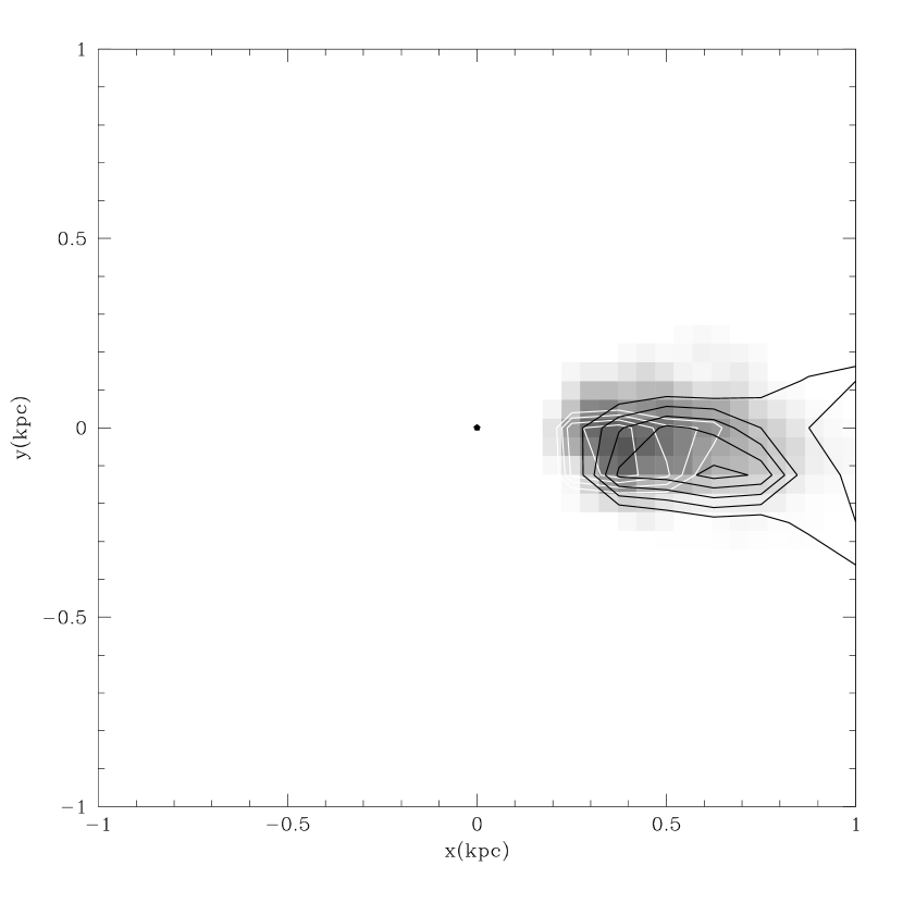
Figure 7: Results of the ram-pressure stripping simulation: gray levels refer to the predicted HI velocity (darker corresponds to more negative values of the velocity) and white contours correspond to heliocentric radial velocities –27, –24, –21 and –18 ${\rm km~{}s}^{-1}$ . The black contours show the predicted gas density (3.5, 3.0, 2.5, 2.0 and 1.5 $\times 10^{19}{\rm cm}^{-2}$)

In Figure 7 we show the results of the simulation: the gray levels refer to the predicted velocity of the gas (darker corresponds to more negative values of the velocity) and the white contours correspond to heliocentric radial velocities –27, –24, –21 and –18 ${\rm km~{}s}^{-1}$ . The black contours correspond to the predicted gas density (3.5, 3.0, 2.5, 2.0 and 1.5 $\times 10^{19}{\rm cm}^{-2}$). The structure of the gas in the simulations remains quite smooth as it is stripped from the satellite, keeping a distribution similar to the observed HI cloud. Note also that a) a velocity gradient in the sense that the most extreme differences in velocity are seen farthest from the galaxy, and b) the velocity of the stripped gas is closer to the systemic velocity of the Milky Way than that of Phoenix are predicted by our model (see also Blitz & Robishaw 2000), in agreement with the observed Phoenix parameters.

These arguments support the hypothesis of the ram-pressure as responsible of the gas stripping in Phoenix. However, it may demand Phoenix to be in its first approach to the Galactic Center, which may be possible if Phoenix is not bound to the MW or it is in a very long period orbit. Given its almost radial orbit, near the pericenter Phoenix must cross zones with a much larger gas density than in its current position, and at much larger velocity with respect to the IGM. This would imply a much larger ram-pressure stripping, to which the gaseous content of the galaxy could have only survived if it originally was very massive and concentrated, unlike at the present time.

There is at least a couple of theoretical works that consider tidal stripping of a gaseous satellite approaching to the Milky Way. They suggest that such a survival in the close approach may not be completely unrealistic. Mayer et al. (1999, 2001) show that low surface brightness satellites of a Milky Way-like galaxy, in eccentric orbits (as typical in hierarchical models of galaxy formation), may lose up to 90% of their stellar mass due to tidal stripping. But, could any amount of gas remain still bound to the galaxy after one or more pericentric passages? Lin & Murray (1999) argue that “around the dSph galaxies in the Galactic halo, their ejected unbound gas follows their orbits analogous to the Magellanic Stream. Gas density declines/enhances near peri/apogalacticon as the stream is stretched/compressed (by tidal forces). At apogalacticon, where the density is at a maximum and exposure to the Galactic UV flux is at a minimum, the diffuse gas can recombine to form atomic and molecular hydrogen and eventually stars”. To assess the plausibility of these different alternatives when ram-pressure is included in the case of Phoenix, it would be necessary to perform much more detailed simulations, which exceed the scope of the present paper. In any case, gas loss will be maximum at the pericenter, where both tidal stripping and ram-pressure forces are larger.

4.2 Comparison with observations of other dwarf galaxies

In two cases, DDO 210 and LGS3 for which HI superimposed to the stellar component had been observed, Blitz & Robishaw (2000) detect a stronger emission component offset from the stellar component. They also find HI possibly associated with Leo I, whose position is also offset from the stellar component. Leo I and LGS3, for which an optical velocity is also known, present interesting similarities with the Phoenix case. In LGS3, HI cloud and galaxy differ in velocity by about 50 ${\rm km~{}s}^{-1}$ , which implies that they are not gravitationally bound. In the case of Leo I, the velocity centroid of the emission that seems more closely associated with the galaxy (both spatially and kinematically) differs by about 30 ${\rm km~{}s}^{-1}$ from the velocity of the stellar component. Apart from the magnitude of the difference in velocity between gas and stars, Leo I, LGS3 and Phoenix are similar also in a) the morphology of the gas relative to the stars and in b) the time of the last events of star formation, which is of the order of a few hundred Myr in all of them (Phoenix: Martínez-Delgado et al. 1999; Leo I: Gallart et al. 1999a,b; LGS3: Aparicio et al. 1997b). For Leo I and LGS3, Blitz & Robishaw (2000) discuss the possibility that the HI has been stripped by the ram-pressure of the hot (Galactic or M31) halo gas. In spite of a distance to the Milky Way of almost twice that of Leo I, this seems a plausible explanation also for Phoenix, as we have discussed in Section 4.1.2.

4.3 Phoenix as a Milky Way satellite, and the mass of the Galaxy

The minimum required mass of the Milky Way for Phoenix to be bound (based on the values of the Galactocentric velocity of Phoenix and its distance to the Galactic center obtained above) is $M_{MW}(<450{\rm kpc})\geq 1.2\times 10^{12}$ M_⊙. This value confortably fits within most current estimates of the Milky Way mass (see Zaritsky 1999 for a review). For example, Zaritsky et al. 1989 conclude that $M_{MW}=(1.3\pm 0.2)\times 10^{12}$ from timing arguments involving Leo I and the Milky Way; on another hand, Anguita, Loyola & Pedreros (2000) calculate, from a recent LMC proper motion measurement that $M_{MW}=(3-4)\times 10^{12}$ out to 50 kpc, if the LMC is to be bound to the Milky Way (see also Méndez et al. 1999). We conclude, therefore, that Phoenix is very likely the outermost (known so far) Milky Way satellite.

5 Summary and conclusions

We present the first measurement of the radial velocity of the Phoenix stellar component, using FORS1 in MOS mode at the VLT UT1 (ANTU) telescope. We have obtained spectra of 31 RGB stars. Two additional stars for which we obtained spectra turned out to be a Carbon star and a bright supergiant star (see Appendix A). From the spectra of the RGB stars we derive an heliocentric optical radial velocity of Phoenix $V_{\odot}=-52\pm 6$ ${\rm km~{}s}^{-1}$ . On the basis of this velocity, and taking into account the results of a series of semi-analytical and numerical simulations, we discuss the possible association of two of the four HI clouds observed in the Phoenix vicinity, those at velocities –23 and $+59$ ${\rm km~{}s}^{-1}$ which are not associated to either the Milky Way or the Magellanic Stream (St-Germain et al. 1999; Young & Lo 1997; Oosterloo et al. 1996).

We conclude that the characteristics (mass, distance, velocity relative to Phoenix) of the HI cloud with heliocentric velocity –23 ${\rm km~{}s}^{-1}$ are consistent with this gas having been associated with Phoenix in the past, until the last event of star formation in the galaxy, about 100 Myr ago. Two possible scenarios for the loss of this gas are discussed: its ejection by the energy released by the SNe produced in that last event of star formation, and a ram-pressure stripping scenario. The assumption that the HI cloud at $+59$ ${\rm km~{}s}^{-1}$ was once associated to Phoenix lead to unlikely boundary conditions (very large number of SNe required or large density of the IGM), which makes us conclude that this one is a chance superposition.

We derive that the kinetic energy necessary to eject the gas is $E_{SNe}\sim 2\times 10^{51}$ erg. The number of SNe necessary to transfer the inferred amount of kinetic energy to the gas cloud is consistent with the total mass involved in the last event of star formation $\sim 100$ Myr ago by Martínez-Delgado et al. (1999). Considering the derived distance between Phoenix and the HI cloud and their relative velocities, the Phoenix total mass necessary for the HI cloud to be gravitationally bound is about an order of magnitude larger than the total mass estimated for Phoenix. This indicates that the amount of energy produced by the last burst of star formation would have been large enough to blow away the small amount of gas remaining in the galaxy after that particular episode of star formation. The main drawbacks of this SNe driven winds scenario is the regular appearance of the HI cloud and its anisotropic distribution with respect to the stellar component. Another possibility is that the HI gas observed at –23 ${\rm km~{}s}^{-1}$ was stripped as a consequence of ram–pressure by the IGM. In our simulations, the structure of the gas remains quite smooth as it is stripped from Phoenix, keeping a distribution similar to that of the observed HI cloud.

Since both the SNe and ram-pressure stripping scenarios for gas ejection in Phoenix are consistent with the observations, a combined scenario may be also plausible. One possibility is that supernovae resulting from a burst of star formation diluted the gas in Phoenix and increased its energy enough for it to be swept away by an already existing intergalactic wind. Another possibility is that Phoenix may be crossing regions of variable gas density, and that 500-100 Myr ago it ran into a relatively dense clump or stream of intergalactic gas that was responsible for the sweeping event that presumably terminated -or temporarily halted- the star formation.

Finally, we discuss the possibility that Phoenix may be a bound Milky Way satellite. The minimum required mass of the Milky Way for Phoenix to be bound is $M_{MW}(<450{\rm kpc})\geq 1.2\times 10^{12}$ M_⊙. This value confortably fits within most current estimates of the Milky Way mass.

Appendix A A young star and a carbon star spectroscopically confirmed (serendipitously) in Phoenix

One of the stars originally selected as a candidate RGB star, Phoenix set#2-6 and Phoenix set#2-10s3 (Table 5) turned out to be other types of stars.

Phoenix set#2-6 (Figure 8a) has the spectra typical of a Carbon star (see for example Cannon, Niss & Norgaard-Nielsen 1980 for a sample spectra and discussion of the features present in a C star spectrum). It is one of the two C stars previously confirmed spectroscopically by Da Costa (1993). It is the brightest red star in our sample, located above the TRGB (identified in the CMD in Figure 4 with a solid square).

Phoenix set#2-10s3 (Figure 8b) was not in our original candidate list. It was included in the extreme of one of the slitlets, and turned out to be a young star. Its spectra clearly shows the series of Balmer lines in absorption, and at this low resolution, low S/N, we can classify it in the range of spectral types B5–A5 (Jacoby, Hunter & Christian 1984). Using (m-M)₀=23.0 and $A_{V}$=0.06 for Phoenix (Martínez-Delgado et al. 1999), the absolute magnitude for this star, if it belongs to Phoenix, is $M_{V}$=-2.83 (Table 5), which would correspond to a bright giant star of luminosity class II, and probably early A spectral type (Landolt-Börnstein 1982). The position of this star in the CMD is consistent with a blue-loop star with Z=0.001 and age 100 Myr, formed in the last event of star formation in Phoenix.

Figure 1: Identification chart for the stars measured in Phoenix. The image is a 120 sec. V exposure at the VLT. North is down and East it to the left.

Figure 2: MOS setup configuration for Phoenix set#1 (Table 1) . FORS1 reference stars are circled. West is up and North is to the left.

Figure 3: MOS setup configuration for Phoenix set#2 (Table 1). FORS1 reference stars are also marked. North is up and East is to the left

Figure 4: CMD of Phoenix with the measured stars near the tip of the red giant branch identified as crosses. The C star and the bright supergiant (late B- early A spectral type) star (see Appendix A) are identified with a filled square and a filled triangle respectively.

Figure 5: Top: Extracted spectrum of a typical Phoenix giant (Phoenix set#1-14 in Table 5). Middle: Spectrum of the master radial velocity template. Bottom: The cross-correlation peak obtained from the top spectrum using the master template. The Tonry-Davis R value for this star is 11.6, which is the median value of all the stars considered in the Phoenix radial velocity derivation

Figure 6: Radial velocities of Phoenix stars as a function of a number of parameters. Clockwise from top left: $V_{r}~{}vs.V$ magnitude, $V_{r}~{}vs.(V-I)$ color index, $V_{r}~{}vs.$ position angle (in degrees), $V_{r}~{}vs.$ galactocentric distance (in arcsec) within Phoenix. Crosses correspond to Phoenix set#1, open circles to Phoenix set#2.1 and solid circles to Phoenix set#2.2. Note that no trends in $V_{r}$ with respect any of these parameters, nor with the Phoenix set, exist.

Figure 8: Top: Spectrum of a Carbon star in Phoenix (Phoenix set#2-6 in Table 5). Bottom: Spectrum of a young star in Phoenix (Phoenix set#2-10s3), probably a bright giant (luminosity class II) of early A spectral type.

Table 1: Observing log for the Phoenix and velocity standard stars

Object	$\alpha_{2000}$	$\delta_{2000}$	ARCHIVE FILE	Exp Time (s)
HD176047#1	18:59:44.12	-34:28:14	FORS.1999-09-14T23:44:30.357.fits	10
HD176047#2	18:59:44.12	-34:28:14	FORS.1999-09-14T23:48:29.001.fits	20
HD176047sky#1	18:59:45.73	-34:28:14	FORS.1999-09-14T23:51:50.492.fits	300
HD176047#3	18:59:44.12	-34:28:14	FORS.1999-09-15T00:00:21.868.fits	150
HD176047sky#2	18:59:45.73	-34:28:14	FORS.1999-09-15T00:06:18.654.fits	600
HD196983#1	20:41:48.98	-33:53:16	FORS.1999-09-15T00:24:57.582.fits	240
HD196983sky#1	20:41:47.44	-33:53:16	FORS.1999-09-15T00:34:39.793.fits	300
HD196983#2	20:41:48.98	-33:53:16	FORS.1999-09-15T01:21:13.492.fits	240
HD196983#3	20:41:48.98	-33:53:16	FORS.1999-09-15T01:28:43.540.fits	120
HD196983sky#2	20:41:50.69	-33:52:57	FORS.1999-09-15T01:34:41.289.fits	600
HD203638	21:24:07.99	-20:50:59	FORS.1999-09-15T03:39:29.409.fits	5
HD203638sky	21:24:09.27	-20:50:59	FORS.1999-09-15T03:42:16.512.fits	600
Phoenix set#1	01:51:04	-44:26:05	FORS.1999-09-15T06:03:47.856.fits	1500
Phoenix set#1	01:51:04	-44:26:05	FORS.1999-09-15T06:30:32.498.fits	1500
Phoenix set#1	01:51:04	-44:26:05	FORS.1999-09-15T06:57:17.324.fits	1500
Phoenix set#2.1	01:50:57	-44:26:40	FORS.1999-09-15T07:34:53.935.fits	1500
Phoenix set#2.1	01:50:57	-44:26:40	FORS.1999-09-15T08:01:38.649.fits	900
Phoenix set#2.2	01:50:57	-44:26:40	FORS.1999-09-15T08:18:01.062.fits	1800
Phoenix set#2.2	01:50:57	-44:26:40	FORS.1999-09-15T08:49:45.413.fits	1800
cpd432597#1	06:32:13.20	-43:31:14	FORS.1999-09-15T09:45:44.645.fits	12
cpd432597#2	06:32:13.20	-43:31:14	FORS.1999-09-15T09:48:03.264.fits	48

Table 2: Radial velocity standards.

Star	$V_{obs}$	R	$\sigma_{v}$	$V_{helio}$	$V_{helio}-V_{obs}$
HD176047#1	-40.8	91.42	4.9	-42.8	-2.0
HD176047#2	-46.1	112.64	4.0	-42.8	3.3
HD176047#3	-42.6	115.85	3.0	-42.8	0.2
HD196983#1	5.2	62.45	7.2	-9.3	-14.5
HD196983#2	-15.2	98.44	4.6	-9.3	5.9
HD196983#3	-10.1	79.65	5.6	-9.3	0.8
HD203638	10.6	63.17	7.1	21.9	11.3

Table 3: Dependence between wavelength zero-point shifts and telescope position. Values for the Phoenix sets are averages over all the slitlets

Object	$\lambda_{obs}$	5577.34 - $\lambda_{obs}$	Alt	Azim
HD176047sky#1	5577.58	-0.24	79.6	342.0
HD176047sky#2	5577.45	-0.11	80.2	358.8
HD196983sky#1	5577.70	-0.36	71.3	304.0
HD196983sky#2	5577.45	-0.11	80.2	342.1
HD203638sky	5577.15	+0.19	73.2	99.4
Phoenix set#1	5577.66	-0.32	67.4	334.4
Phoenix set#2.1	5577.05	+0.29	68.8	18.8
Phoenix set#2.2	5577.08	+0.26	64.3	34.6

Table 4: Summary of repeat velocity measurements

Star	$V_{helio}$	$R$	$<V>$	$V_{helio}-<v>$
HD176047#1	-40.8	91.4	-43.2	2.4
HD176047#2	-46.1	112.6	-43.2	-2.9
HD176047#3	-42.6	115.8	-43.2	0.5
HD196983#1	5.2	62.4	-6.7	11.9
HD196983#2	-15.2	98.4	-6.7	-8.5
HD196983#3	-10.2	79.6	-6.7	-3.4
Phoenix set#2.1-5	-54.6	8.8	-66.3	11.61
Phoenix set#2.2-5	-77.9	13.4	-66.3	-11.61
Phoenix set#2.1-8	-26.3	10.4	-47.3	21.01
Phoenix set#2.2-8	-68.3	15.4	-47.3	-21.01
Phoenix set#2.1-9	-51.5	8.1	-52.3	0.80
Phoenix set#2.2-9	-53.1	21.1	-52.3	-0.80
Phoenix set#2.1-12	-68.0	9.1	-53.9	-14.1
Phoenix set#2.2-12	-39.9	13.9	-53.9	14.1
Phoenix set#2.1-14	-9.3	9.0	-28.3	19.0
Phoenix set#2.2-14	-47.3	18.2	-28.3	-19.0
Phoenix set#2.1-15	-30.0	9.8	-44.8	14.8
Phoenix set#2.2-15	-59.6	14.5	-44.8	-14.8

Table 5: Data of the spectroscopically observed stars in Phoenix, with radial velocities for the RGB stars with sufficient S/N to obtain a well defined cross-correlation peak.

Star	$\alpha_{2000}$	$\delta_{2000}$	$V$	$v_{helio_{obs}}$	$R$	$\sigma_{v}$	Comment
Phoenix set#1-5	01:50:53.4	-44:25:34.6	21.03	-64.1	10.1	40.9
Phoenix set#1-6	01:50:55.4	-44:26:43.7	20.71	-60.1	16.9	25.4
Phoenix set#1-7	01:50:58.1	-44:26:47.7	21.13	-23.7	9.8	42.2
Phoenix set#1-8	01:50:59.7	-44:26:18.0	21.24	-64.7	17.4	24.7
Phoenix set#1-9	01:51:02.0	-44:26:15.3	20.94	-84.7	18.9	22.8
Phoenix set#1-10	01:51:04.1	-44:27:16.6	20.70	-78.3	16.3	26.3
Phoenix set#1-11	01:51:06.5	-44:26:36.3	20.60	-38.4	27.1	16.2
Phoenix set#1-12	01:51:08.1	-44:27:03.9	20.76	-57.2	16.7	25.6
Phoenix set#1-13	01:51:10.7	-44:26:04.8	20.70	-39.0	9.7	42.5
Phoenix set#1-14	01:51:12.5	-44:27:04.6	21.38	-52.1	11.6	36.1
Phoenix set#1-15	01:51:14.9	-44:25:41.8	21.02	-68.9	21.3	20.4
Phoenix set#1-16	01:51:17.1	-44:26:01.2	20.82	-52.0	9.7	42.4
Phoenix set#1-17	01:51:19.2	-44:26:34.3	20.71	–	–	–	Low S/N
Phoenix set#1-18	01:51:21.2	-44:26:03.1	21.05	–	–	–	Low S/N
Phoenix set#2.2-2	01:51:05.1	-44:29:42.6	21.33	-52.9	8.8	46.2
Phoenix set#2.2-3	01:51:07.3	-44:29:23.5	21.06	-74.6	8.7	47.0
Phoenix set#2.2-4	01:51:09.6	-44:29:03.1	20.95	-59.2	7.4	54.0
Phoenix set#2.1-5	01:51:08.3	-44:28:30.7	20.88	-48.5	8.8	46.2
Phoenix set#2.2-5				-77.6	13.4	31.5
Phoenix set#2.2-6	01:51:08.9	-44:28:11.9	20.62	–	–	–	C star
Phoenix set#2.2-7	01:51:10.2	-44:27:48.2	21.21	-19.3	16.6	25.9
Phoenix set#2.1-8	01:51:06.7	-44:27:22.8	20.73	-26.4	10.5	39.4
Phoenix set#2.2-8				-66.3	15.6	27.3
Phoenix set#2.1-9	01:51:08.1	-44:27:03.9	20.72	-50.8	8.2	49.3
Phoenix set#2.2-9				-51.9	21.4	20.3
Phoenix set#2.2-10	01:51:02.8	-44:26:45.5	21.03	-92.1	16.1	26.7
Phoenix set#2.2-10;s2	01:51:02.8	-44:26:41.9	21.34	-67.0	14.9	28.6
Phoenix set#2.2-10;s3	01:51:02.7	-44:26:32.3	20.23	–	–	–	bright supergiant
Phoenix set#2.2-11	01:51:10.8	-44:26:23.9	20.93	-48.3	8.3	48.9
Phoenix set#2.2-11;s2	01:51:10.8	-44:26:20.5	21.72	-88.6	13.8	30.7
Phoenix set#2.1-12	01:51:05.6	-44:25:52.4	20.85	-68.6	9.1	45.1
Phoenix set#2.2-12				-39.3	13.8	30.7
Phoenix set#2.2-13	01:51:08.3	-44:25:34.4	21.27	-51.5	8.8	46.3
Phoenix set#2.1-14	01:51:04.9	-44:25:10.5	20.78	-15.8	9.2	44.4
Phoenix set#2.2-14				-46.1	18.6	23.3
Phoenix set#2.2-15	01:51:04.4	-44:24:42.9	20.72	-58.7	14.4	29.5
Phoenix set#2.2-16	01:51:10.8	-44:24:24.3	21.33	-44.7	7.9	51.3
Phoenix set#2.1-18	01:51:12.9	-44:23:41.4	20.61	-41.1	7.7	52.2
Phoenix set#2.2-18				-50.8	9.9	41.7

References

- (1)
- (2) Anguita, C., Loyola, P. & Pedreros, M. 2000, AJ, 120, 845
- (3)
- (4) Aparicio, A., Gallart, C. & Bertelli, G. 1997a, AJ, 114, 669
- (5)
- (6) Aparicio, A., Gallart, C. & Bertelli, G. 1997b, AJ, 114, 680
- (7)
- (8) Bingelli, B. 1993, in “Panchromatic View of Galaxies”, eds. G. Hensler, Ch. Theis & J. Gallagher. Éditions Frontières, Gif-sur-Yvette, p. 173
- (9)
- (10) Blitz, L. & Robishaw, T. 2000 ApJ, submitted (astro-ph0001142)
- (11)
- (12) Carignan, C., Demers, S. & Côté, S. 1991, ApJ, 381, L13
- (13)
- (14) Carignan, C., Beaulieu, S., Côté, S., Demers, S., Mateo. M. 1998, AJ, 116, 1690
- (15)
- (16) Cannon, R.D., Niss, B. & Norgaard-Nielsen, H.U. 1980, MNRAS, 196, Short Comm, 1.
- (17)
- (18) Da Costa, G.S. 1993, in “ Proceedings of the ESO/OHP Workshop on Dwarf Galaxies”, eds. G. Meylan & P. Prugniel, ESO Conference and Workshop Proceedings No. 49.
- (19)
- (20) Davies, J.I. & Phillips, S. 1989, Ap&SS, 157, 291
- (21)
- (22) Dekel, A. & Silk, J. 1986, ApJ, 303, 39
- (23)
- (24) Einasto, J., Saar, E., Kaasik, A. & Chernin, A.D. 1974, Nature, 252, 111
- (25)
- (26) Ferrara, A. & Tolstoy, E. 2000, MNRAS, 313, 291
- (27)
- (28) Gallart, C., Freedman, W.L., Mateo, M., Chiosi, C., Thompson, I.B., Aparicio, A., Bertelli, G., Hodge, P., Lee, M.Y., Olsewszki, E.O., Saha, A., Stetson, P.B. & Suntzeff, N. 1999a, ApJ, 514, 665
- (29)
- (30) Gallart, C., Freedman, W.L., Aparicio, A., Bertelli, G. & Chiosi, C. 1999b, AJ, 118, 2245
- (31)
- (32) Gómez-Flechoso, M.A. 2000, in preparation.
- (33)
- (34) Gunn, J.E. & Gott, J.R. 1972, ApJ, 176, 1
- (35)
- (36) Held, E.V., Saviane, I. & Momany, Y. 1999, A&A, 345, 747
- (37)
- (38) Jacoby, G.H., Hunter, D.A. & Christian, C.A. 1984, ApJS, 56, 257
- (39)
- (40) Kroupa, P., Tout, C.A. & Gilmore, G. 1993, MNRAS, 262, 545
- (41)
- (42) Lacey, C. & Silk, J. 1991, ApJ, 381, 14
- (43)
- (44) Landolt-Börnstein, Vol 2b. Eds. K. Schaifers & H.H. Voigt, Springer-Verlag Berlin, Heidelberg, New York 1982
- (45)
- (46) Larson, R. 1974, MNRAS, 169, 229
- (47)
- (48) Lin, D.N.C. & Faber, S.M. 1983, ApJ, 266, L21
- (49)
- (50) Lin, D.N.C. & Murray, S.D. 1998, in Dwarf galaxies and Cosmology, Eds. T.X. Thuan, C. Balkowski, V. Cayatte, and J.T.T. Van, Eds Frontières.
- (51)
- (52) Lo, K.Y., Sargent, W.L.W. & Young, K., 1993, AJ, 106, 507
- (53)
- (54) Mac Low, M.-M. & Ferrara, A. 19999, ApJ, 513, 142
- (55)
- (56) Martínez-Delgado, D., Gallart, C. & Aparicio, A. 1999, AJ, 118, 862
- (57)
- (58) Mateo, M. 1998, ARA&A, 36, 435
- (59)
- (60) Mathews, W.G. & Baker, J.C. 1971, ApJ, 170, 241
- (61)
- (62) Maurice, E. et al. 1984, A&AS, 57, 275
- (63)
- (64) Mayer, L., Governato, F., Colpi, M., Moore, B., Quinn, T.R. & Baugh, C.M. 1999, astro-ph/9903442
- (65)
- (66) Mayer, L., Governato, F., Colpi, M., Moore, B., Quinn, T.R., Wadsley, J., Stadel, J. & Lake, G. 2001, ApJ, in press
- (67)
- (68) Méndez, R. A., Platais, I., Girard, T.M., Kozhurina-Platais, V. & van Altena, W.F. 1999, ApJ, 524, L39
- (69)
- (70) Mulchaey, J.S. 2000, ARA&A, 38, 289
- (71)
- (72) Murali, C. 2000, ApJ, 529, L81
- (73)
- (74) Oosterloo, T., Da Costa, G.S., Staveley-Smith, L. 1996, AJ, 112, 1969
- (75) Osterbrock, D. E., Fulbright, J.P., Martel, A.R., Keane, M.J. & Trager, S.C. 1996, PASP, 108, 277
- (76)
- (77) Puche, D. & Westpfahl, D. 1993, in Proceedings of the ESO/OHP workshop on Dwarf Galaxies, Eds. G. Meylan & P. Prugniel. ESO Conference and Workshop Proceedings No. 49, p. 273.
- (78)
- (79) Silk, J. Wyse, R.F.G. & Shields, G.A. 1987, ApJ, 322, L59
- (80)
- (81) Smecker-Hane, T.A., Stetson, P.B., Hesser, J.E. & Lehnert, M.D. 1994, AJ, 108, 507
- (82) Stetson, P. B., Hesser, J.E. & Smecker-Hane, T.A. 1998, PASP, 110, 533
- (83)
- (84) St-Germain, J., Carignan, C., Côté, S. & Oosterloo, T. 1999, AJ, 1235, 1244
- (85)
- (86) Suto, Y., Makishima, K., Ishisaki, Y. & Ogasaka, Y. 1996, ApJ, 461, L33
- (87)
- (88) Tonry, J. & Davis, M. 1979, AJ, 84, 1511
- (89)
- (90) van den Bergh, S. 1994, ApJ, 428, 617
- (91)
- (92) Vogt, S.S., Mateo, M., Olszewski, E.W. & Keane, M.K. 1995, AJ, 109, 151
- (93)
- (94) Young, L.M. & Lo, K.Y. 1997, ApJ, 490, 710
- (95)
- (96) Zaritsky, D. 1999, in ASP Conf. Ser. 165, The Third Stromlo Symp.: “The Galactic Halo”, ed. B.K. Gibson, T.S. Axelrod & M.E. Putnam (San Francisco: ASP), 34
- (97)
- (98) Zaritsky, D., Olszewski, E.W., Schommer, R.A., Peterson, R.C. & Aaronson, M. 1989, ApJ, 345, 759
- (99)