Structure of gaseous flows in semidetached binaries after mass transfer termination

Abstract

The results of three-dimensional numerical simulations of mass transfer in semidetached binaries after mass transfer termination is presented and the structure of residual accretion disk was investigated. It was shown that after the mass transfer termination the quasi-elliptic accretion disk becomes circular. It was also shown that the cessation of mass transfer results in changing of the structure of the accretion disk: the second arm of spiral shock is appeared as well as a new dense formation (blob), the latter moving through the disk with variable velocity. The blob doesn’t smear out under the action of dissipation but is sustained by interaction with arms of spiral shock for practically all the lifetime of the disk.

We also analyze the dependence of disk’s lifetime on the value of viscosity. For the value of parameter $\alpha$ that is typical for observing accretion disk ($\alpha\sim 0.01$) the lifetime of residual disk is found to be equal to 50 orbital periods.

1 Introduction

Semidetached binaries are known to be interacting binary stars in which one component fills its Roche lobe and looses mass through the vicinity of inner Lagrangian point $L_{1}$. Earlier we developed the 3D gasdynamical model for simulation of the mass transfer in semidetached binaries (see Bisikalo et al. 1997${}^{\cite[cite]{[\@@bibref{}{dima97}{}{}]}}$, 1998b${}^{\cite[cite]{[\@@bibref{}{dima98b}{}{}]}}$, 1998c${}^{\cite[cite]{[\@@bibref{}{dima98c}{}{}]}}$). When applying to binaries with constant mass transfer rate this model allows to determine the main features of flow structure (see Bisikalo et al. 1997${}^{\cite[cite]{[\@@bibref{}{dima97}{}{}]}}$, 1998b${}^{\cite[cite]{[\@@bibref{}{dima98b}{}{}]}}$, 1998c${}^{\cite[cite]{[\@@bibref{}{dima98c}{}{}]}}$, 1999${}^{\cite[cite]{[\@@bibref{}{dima99}{}{}]}}$, 2000${}^{\cite[cite]{[\@@bibref{}{dima2000}{}{}]}}$). In particular, the stream interaction is shown to be shock-free for steady-state regime of the flow and the model of ‘hot line’ was introduced for binaries with constant rate of mass transfer instead traditional ‘hot spot’ model. Successful application of the ‘hot line’ model for analysis of light curves in cataclysmic variables (Bisikalo et al. 1998a${}^{\cite[cite]{[\@@bibref{}{dima98a}{}{}]}}$; Khruzina et al. 2001${}^{\cite[cite]{[\@@bibref{}{tanya2001}{}{}]}}$) allows us to conclude that the model appears to be adequate for considered systems.

On the other hand, some observations show that for a large number of semidetached binaries there exist both epochs of constant rate of mass transfer and epochs in which the rate of mass transfer changes considerably (see, e.g., Bath et al. 1974${}^{\cite[cite]{[\@@bibref{}{bath74}{}{}]}}$; Wood 1977${}^{\cite[cite]{[\@@bibref{}{wood77}{}{}]}}$; Bath & Pringle 1982${}^{\cite[cite]{[\@@bibref{}{bath81}{}{}]}}$; Bath & van Paradijs 1983${}^{\cite[cite]{[\@@bibref{}{bath83}{}{}]}}$; Gilliland 1985${}^{\cite[cite]{[\@@bibref{}{gilliland85}{}{}]}}$; Ritter 1988${}^{\cite[cite]{[\@@bibref{}{ritter88}{}{}]}}$; Murray, Warner & Wickramasinghe 2000${}^{\cite[cite]{[\@@bibref{}{murray2000}{}{}]}}$; Schreiber, Gänsicke & Hessman 2000${}^{\cite[cite]{[\@@bibref{}{schreiber2000}{}{}]}}$). Evolutionary scenarios also predict the possibility of the contraction of the mass-losing star. In this case the star doesn’t fill the Roche lobe anymore and mass transfer will be terminated.

The purpose of this paper is to investigate the flow structure in a semidetached binary after the mass transfer termination. On the first stage we have conducted 3D gasdynamical simulation of mass transfer for the case of constant rate of mass transfer up to the steady-state solution. Then we adopt that matter outflow is ceased and consider the structure of residual disk. It is clear that the evolution of accretion disk is controlled by physical processes responsible for the redistribution of the angular momentum in the disk. To investigate the influence of viscosity we conduct 3 runs for various values of viscosity, these ones corresponding to following values of parameter $\alpha$ (in terms of the $\alpha$-disk): $\alpha\sim 0.08\div 0.1$, $\alpha\sim 0.04\div 0.06$, and $\alpha\sim 0.01\div 0.02$.

2 Statement of the problem

Let us consider a semidetached binary system and adopt that accretor has the mass $M_{1}$, the mass-donating star has the mass $M_{2}$, the separation of the binary system is $A$, and angular velocity of orbital rotation is $\Omega$. The flow of matter in this system can be described by Euler equations with equation of state for ideal gas $P=(\gamma-1)\rho\varepsilon$, where $P$ – pressure, $\rho$ – density, $\varepsilon$ – specific internal energy, $\gamma$ – adiabatic index. To mimic the radiative loss of energy we adopt the value of $\gamma$ close to 1: $\gamma=1.01$, which corresponds to the near-isothermic case (Sawada, Matsuda & Hachisu 1986${}^{\cite[cite]{[\@@bibref{}{spiral1}{}{}]}}$; Molteni, Belvedere & Lanzafame 1991${}^{\cite[cite]{[\@@bibref{}{diego91}{}{}]}}$; Bisikalo et al. 1997${}^{\cite[cite]{[\@@bibref{}{dima97}{}{}]}}$).

To obtain the numerical solution of the system of equations we used the Roe–Osher TVD scheme of a high approximation order (Roe 1986${}^{\cite[cite]{[\@@bibref{}{roe86}{}{}]}}$; Chakravarthy & Osher 1985${}^{\cite[cite]{[\@@bibref{}{osher85}{}{}]}}$) with Einfeldt modification (Einfeldt 1988${}^{\cite[cite]{[\@@bibref{}{einfeldt88}{}{}]}}$). The original system of equations were written in a dimensionless form. To do this, the spatial variables were normalized to the distance between the components $A$, the time variables were normalized to the reciprocal angular velocity of the system ${\Omega}^{-1}$, and the density was normalized to its value in the inner Lagrangian point $L_{1}$. The gas flow was simulated over a parallelepipedon $[\hbox{$\,{}^{1}\!/_{2}$}A\ldots\hbox{$\,{}^{3}\!/_{2}$}A]\times[-\hbox{$\,{}^{1}\!/_{2}$}A\ldots\hbox{$\,{}^{1}\!/_{2}$}A]\times[0\ldots\hbox{$\,{}^{1}\!/_{4}$}A]$ (calculations were conducted only in the top half-space). The sphere with a radius of $\hbox{$\,{}^{1}\!/_{100}$}A$ representing the accretor was cut out of the calculation domain.

The boundary and the initial conditions were determined as follows: (i) we adopted free-outflow conditions at the accretor and at the outer boundary of the calculation domain; (ii) on the first stage in gridpoint corresponding to $L_{1}$ we injected the matter with parameters $\rho=\rho(L_{1})$, $V_{x}=c(L_{1})$, $V_{y}=V_{z}=0$, where $c(L_{1})$ is a gas speed of sound in $L_{1}$ point; (iii) for this stage we used rarefied background gas with the following parameters $\rho_{0}=10^{-5}\cdot\rho(L_{1})$, $P_{0}=10^{-4}\rho(L_{1})c^{2}(L_{1})/\gamma$, ${{\mathchoice{\hbox{$\displaystyle V$}}{\hbox{$\textstyle V$}}{\hbox{$\scriptstyle V$}}{\hbox{$\scriptscriptstyle V$}}}}_{0}=0$ as the initial conditions; (iv) on the second stage when steady-state regime is reached at the moment of time $t=t_{0}$ we decreased the density of the injected matter to the value $\rho=\rho_{0}$.

The analysis of considered problem shows that the gas dynamical solution for the semidetached binary is defined by three dimensionless parameters (Bisikalo et al. 1998b${}^{\cite[cite]{[\@@bibref{}{dima98b}{}{}]}}$, 1999${}^{\cite[cite]{[\@@bibref{}{dima99}{}{}]}}$; Lubow & Shu 1975${}^{\cite[cite]{[\@@bibref{}{lubowshu75}{}{}]}}$): the mass ratio $q=M_{2}/M_{1}$, the Lubow-Shu parameter $\epsilon=c(L_{1})/A\Omega$ (Lubow & Shu 1975${}^{\cite[cite]{[\@@bibref{}{lubowshu75}{}{}]}}$), and the adiabatic index $\gamma$. The value of the adiabatic index was discussed above and we used the value $\gamma=1.01$. Analysis of our previous results (Bisikalo et al. 1998b${}^{\cite[cite]{[\@@bibref{}{dima98b}{}{}]}}$, 1999${}^{\cite[cite]{[\@@bibref{}{dima99}{}{}]}}$) shows that the main characteristic features of 3D gas dynamical flow structure are qualitatively the same in wide range of parameters $q$ and $\epsilon$. Therefore for the model simulation we chose them as follows: $q=1$, $\epsilon=\hbox{$\,{}^{1}\!/_{10}$}$.

To evaluate the influence of the viscosity on the solution, several runs with different spatial resolution were conducted. The Euler equations do not include physical viscosity so we varied the numerical viscosity by virtue of changing of computational grid. Three grids were chosen for simulation: $31\times 31\times 17$, $61\times 61\times 17$, $91\times 91\times 25$ (hereinafter runs ”A”, ”B”, and ”C”, correspondingly). In terms of the $\alpha$-disk the numerical viscosity for runs ”A”, ”B”, ”C” approximately corresponds $\alpha\sim 0.08\div 0.1$, $\alpha\sim 0.04\div 0.06$, and $\alpha\sim 0.01\div 0.02$.

3 Flow structure after the mass transfer termination

Prior to simulation of the flow structure with ‘turned-off’ mass transfer the near-steady-state solutions for the case of constant non-zero rate of mass transfer were obtained (Bisikalo et al. 2000${}^{\cite[cite]{[\@@bibref{}{dima2000}{}{}]}}$) and used as initial conditions. At the moment of time $t=t_{0}$ the rate of mass transfer was decreased in five order of magnitude, which is correspond to the cessation of mass transfer.

Calculations of runs ”A” and ”B” were lasted until the density of gas becomes less than the background density $\rho_{0}=10^{-5}\rho(L_{1})$. This corresponds to the full vanishing of matter due to accretion and outflow through outer boundary. The durations of these two runs correspond to $5P_{orb}$ and $12P_{orb}$ after the moment of time $t_{0}$. Run ”C” has the best resolution and minimal numerical viscosity. Nevertheless this run was conducted to $10P_{orb}$ only, since this run is very computer-time-consuming while the time when disk vanishes can be estimated as $\sim 50P_{orb}$. We extrapolated the results of calculation of run ”C” for $t>10P_{orb}$.

Figure 1: Time evolution of the total mass of the calculation domain (top part of the figure) and the mass of the disk (bottom part of the figure) for ”A”, ”B”, and ”C” runs. The mass of uniform matter with background density $\rho=\rho_{0}$ for the whole computation domain and for the disk are shown by dashed lines.

Before investigating of the structure of gaseous flows in binary system let us estimate the lifetime of the residual disk after the termination of mass transfer for different values of viscosity. The lifetime of the residual disk can be evaluated from the Fig. 1 where the total mass of the calculation domain (top part of the figure) and the mass of the disk (bottom part of the figure) versus time is presented. The lower limit of the density of gas is the background density $\rho_{0}$, therefore the mass of the uniform matter with $\rho=\rho_{0}$ calculated for the whole computation domain and for the disk are asymptotic lines for graphs $M(t)$. These lines are shown in the Fig. 1 by dashed lines.

The analysis of the data presented in the Fig. 1 shows (and there is no surprise now) that the lifetime of the residual disk is increased when the numerical viscosity is decreased: for run ”A” ($\alpha\sim 0.1$) $\tau_{disk}=5P_{orb}$; for run ”B” ($\alpha\sim 0.05$) $\tau_{disk}=12P_{orb}$; and for run ”C” ($\alpha\sim 0.05$) the extrapolation of the result of simulation shows that the lifetime of the residual disk exceeds $50P_{orb}$. It is pertinent to note that the value $\alpha\sim 0.01$ is typical for observable accretion disks (see, e.g., Lynden-Bell & Pringle 1974${}^{\cite[cite]{[\@@bibref{}{lyndenbell74}{}{}]}}$; Meyer-Hofmeister & Ritter 1993${}^{\cite[cite]{[\@@bibref{}{meyer93}{}{}]}}$; Armitage & Livio 1996${}^{\cite[cite]{[\@@bibref{}{armi96}{}{}]}}$; Tout 1996${}^{\cite[cite]{[\@@bibref{}{tout96}{}{}]}}$). Consequently, we can expect the lifetime of residual disk after the termination of mass is of order $50P_{orb}$ (near a week) for typical dwarf novae.

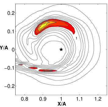
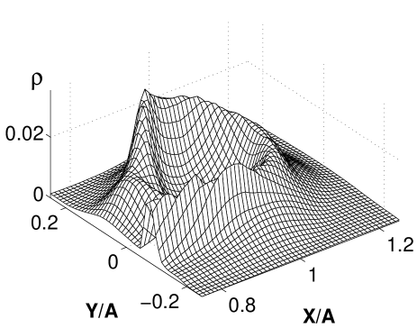
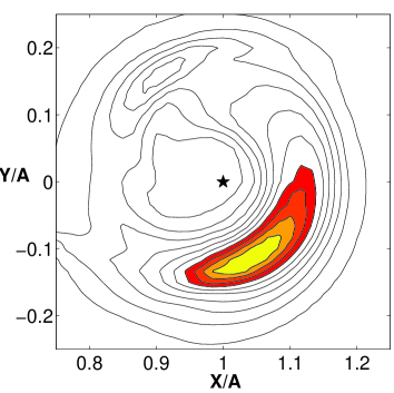
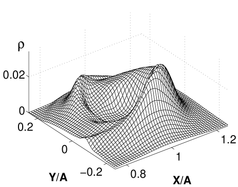
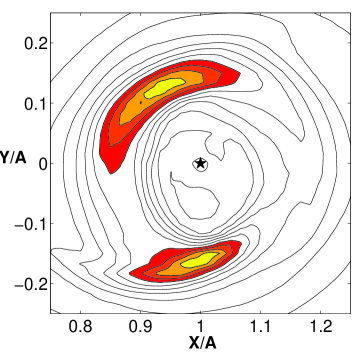
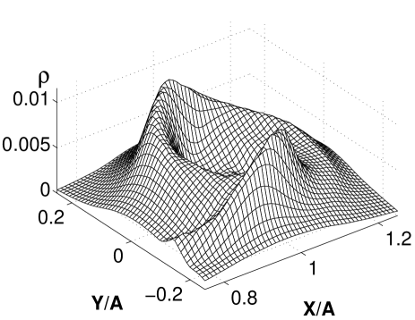
Figure 2: Isolines (left panels) and bird-eye vies (right panels) of density in the equatorial plane. Three rows of panels correspond to the following moments of time: $t=t_{0}+0.08P_{orb}$, $t=t_{0}+0.16P_{orb}$, $t=t_{0}+0.9P_{orb}$, where $t_{0}$ is the moment of the mass transfer termination.

Now let us consider the evolution of the residual accretion disk in time. Since the results of runs ”A”, ”B”, ”C” are qualitatively similar, we will focus on the run ”B” and analyze it in detail. The choice of run ”B” is called forth by the following reasons: firstly, the spatial resolution of this run is well enough to catch all the details of the disk structure, and, secondly, the lifetime of residual accretion disk is sufficiently small ($12P_{orb}$) so we can study its fate up to full vanishing. The Figure 2 presents isolines and bird-eye views of density in the equatorial plane for different moments of time. the upper panels correspond to the moment of time $t=t_{0}+0.08P_{orb}$, middle panels – to $t=t_{0}+0.16P_{orb}$, and lower panels – to $t=t_{0}+0.9P_{orb}$. The analysis of these figures shows that for initial moments of time ($t<t_{0}+0.08P_{orb}$) the structure of accretion disk doesn’t differ much from the structure obtained for the steady-state solution with constant mass transfer rate (see Bisikalo et al. 1997${}^{\cite[cite]{[\@@bibref{}{dima97}{}{}]}}$, 1998b${}^{\cite[cite]{[\@@bibref{}{dima98b}{}{}]}}$, 1998c${}^{\cite[cite]{[\@@bibref{}{dima98c}{}{}]}}$, 1999${}^{\cite[cite]{[\@@bibref{}{dima99}{}{}]}}$, 2000${}^{\cite[cite]{[\@@bibref{}{dima2000}{}{}]}}$). As always the stream of matter from $L_{1}$ dominates. It is clearly seen that the uniform morphology of the system stream–disk results in quasi-elliptical shape of the disk and the absence of ‘hot spot’ in zone of stream–disk interaction. At the same time the interaction of the gas of circumbinary envelope with the stream results in the formation of an extended shock wave located along the stream edge (‘hot line’). The Figure 2 also manifests the formation of tidally induced spiral shock located in I and II quadrants of coordinate plane. Appearance of tidally induced two-armed spiral shock was discovered in Sawada et al. (1986a${}^{\cite[cite]{[\@@bibref{}{spiral1}{}{}]}}$, 1986b${}^{\cite[cite]{[\@@bibref{}{spiral2}{}{}]}}$, 1987${}^{\cite[cite]{[\@@bibref{}{sawada87}{}{}]}}$). Here we see only the one-armed spiral shock. The flow structure in the place where the second arm should be is defined by the stream from $L_{1}$ which appears to suppress the formation of another arm of the tidally induced spiral shock.

Figure 3: Time variation of the mean density of matter passing through a semi-plane $XZ$ ($Y=0$, $X>A$) slicing the disk. A zoom for the mean density variation for times from $t_{0}$ to $t_{0}+1.4P_{orb}$ is shown in the top of the figure. Two sets of moments of time (8 moments per set, each set covers one period of the mean density variation) are also shown.

From the panels of middle row of the Fig. 2 it is seen that after the moment of time $t\sim t_{0}+0.16P_{orb}$ the stream from $L_{1}$ has no influence on the structure of residual accretion disk anymore and the disk is circularized. It is also seen that the shock wave located along the stream edge (‘hot line’) disappears and the second arm of the tidally induced spiral shock located in III and IV quadrants of coordinate plane is formed. It is illustrated by lower row of the Fig. 2 where results of simulations for the moment of time $t=t_{0}+0.16P_{orb}$ are presented. Note that the intensity of shocks as well as the mass of accretion disk decreased in time but the qualitative flow structure retains. The flow structure is changed when the tidal interaction doesn’t result in the formation of spiral shocks anymore (it corresponds to the moments of time $t_{0}+10P_{orb}\div t_{0}+11P_{orb}$ for run ”B”). Therefore, we can conclude that the spiral shocks exists during of all lifetime of the disk (remind that it is of order $12P_{orb}$ for run ”B”).

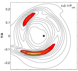
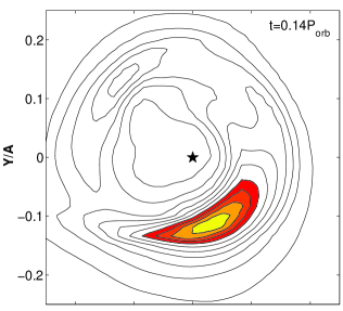
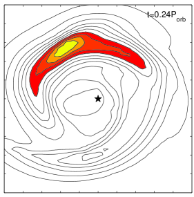
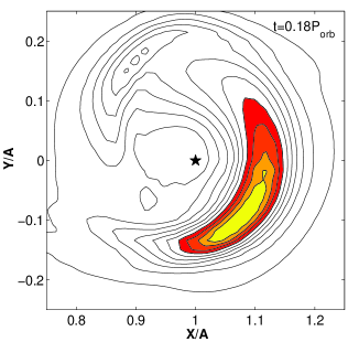
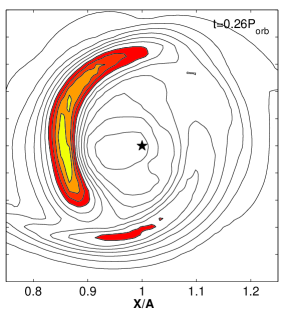
Figure 4a: Density distribution in the equatorial plane for the first set of moments of time from Fig. 3.

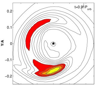
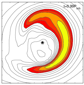
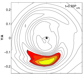
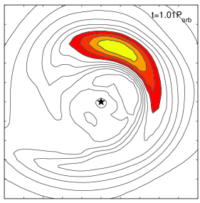
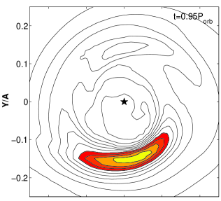
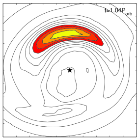
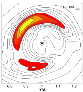
Figure 4b: Density distribution in the equatorial plane for the second set of moments of time from Fig. 3.

Our results also show the formation of dense blob in the residual disk. The blob is formed after the stream vanishes, i.e. after time $\sim t_{0}+0.15P_{orb}$ and rotates with variable velocity. The Figure 3 presents time variation of the mean density of matter passing through a semi-plane $XZ$ ($Y=0$, $X>A$) slicing the disk. Along with a general density fall we can see here periodic oscillations called forth by passing the blob. The blob doesn’t smear out under the action of dissipation and the period of its rotation ($\sim 0.18P_{orb}$) remains the same practically up to the moment when the disk vanishes. Figure 3 also contains a zoom for the mean density variation for times from $t_{0}$ to $t_{0}+1.4P_{orb}$. Here we marked 2 sets of moments of time (8 moments per set), each set covering one period of the mean density variation. The first set corresponds to the moments of time $t_{0}+0.11P_{orb}\div t_{0}+0.26P_{orb}$, and the second – to $t_{0}+0.91P_{orb}\div t_{0}+1.06P_{orb}$. Figures 4a and 4b show the density distributions for the moments of time of these two sets. Analysis of the data of Fig. 4a,b, shows that the blob retains by its interaction with the arms if spiral shocks.

Let us consider this mechanism in detail. Initially appearing as the residue of the stream, the blob tends to distribute uniformly along the disk under the action of dissipation but retards after passing trough spiral shock so the compactness of the blob retains. Later the increasing density contrast between the blob and the disk and growths of pressure gradient will force the standstilled blob to move. When reaching the second arm of spiral shock the process of formation/retainment of the blob is repeated. This mechanism is confirmed by data of Fig. 5. Figure 5a presents the velocity of the blob (the velocity of the point with maximal density) versus time (solid line). The keplerian velocity of this point $V_{K}=\sqrt{GM_{1}/r}$ is also shown by dashed line. The velocity variations are shown for time interval $t_{0}+0.91P_{orb}\div t_{0}+1.11P_{orb}$ including the time interval for Fig. 4b and covering the full period of blob’s revolution. Figure 5b shows variation of maximal density in the equatorial plane for the same time interval. It is seen from Fig. 5 that matter is retarded after passing the shock and becomes more dense, the maximal density $\rho_{max}$ being increased 1.5 times. When accumulating a sufficient amount of matter, the blob comes off the shock and its velocity increases while maximal density decreases. After passing the second arm of spiral shock the blob is retarded again. Note that the contrast of density between the blob and the disk remains the same up to the moment when the blob disappears. In this moment of time the disk is contracted and spiral shock disappears as well. Later the density contrast blob/disk decreases under the action of dissipation but the blob exists up to the full vanishing of the disk. This is illustrated in Fig. 6 where time dependency of the density contrast blob/disk is shown. The large value of density contrast as well as the variable velocity of the blob revolution (but with constant period $\sim 0.18P_{orb}$) make this feature very interesting for observations.

Figure 5: Upper panel: A solid line – variation of the velocity of the blob (the velocity of the point with maximal density). A dashed line – keplerian velocity of this point $V_{K}=\sqrt{GM_{1}/r}$. The velocity variations are shown for time interval $t_{0}+0.91P_{orb}\div t_{0}+1.11P_{orb}$ including the time interval for Fig. 4b and covering the full period of blob’s revolution.
Lower panel: Variation of the maximal density of the blob.

Figure 6: The density contrast between the disk and the blob versus time.

4 Conclusions

We have presented the results of 3D numerical simulations of mass transfer in semidetached binaries after the mass transfer termination. Prior to simulation of flow structure with ‘turned-off’ mass transfer the near-steady-state solutions for the case of constant non-zero rate of mass transfer was obtained and used as the initial conditions. At the moment of time $t=t_{0}$ the rate of mass transfer was decreased in five order of magnitude, which corresponds to the cessation of mass transfer. To investigate the influence of the viscosity we conduct 3 runs for various values of viscosity, corresponding to following values of parameter $\alpha$ (in terms of $\alpha$-disk): $\alpha\sim 0.08\div 0.1$, $\alpha\sim 0.04\div 0.06$, and $\alpha\sim 0.01\div 0.02$.

The investigation of structure of the residual disk reveals an essential increasing of its lifetime when the viscosity deceases. Even for $\alpha\sim 0.05$ the lifetime of residual disk exceeds $12P_{orb}$, and for $\alpha\sim 0.01$ (that is typical for observable accretion disks) the lifetime of residual disk is as much as $50P_{orb}$.

Our simulations show that near the moment of time $t=t_{0}+0.2P_{orb}$ the flow structure is changed significantly. The stream from $L_{1}$ doesn’t dominate anymore, and the shape of accretion disk changes from quasi-elliptical to circular. The second arm of tidally induced spiral shock is formed while earlier (before the termination of mass transfer) it was suppressed by the stream from $L_{1}$. The mass of the disk is gradually decreased but spiral shocks exist practically up to the full vanishing of the disk.

Our simulations also show that a dense blob is formed in the residual disk, the velocity of the blob motion through the disk being variable. The blob doesn’t smear out under the action of dissipation but is sustained by interaction with arms of spiral shock up to the moment of time when spiral shock disappears. The density contrast between the blob and the disk is rather large $\sim 1.6$ and begins to decrease only when spiral shock disappears (it occurs at time $\sim t_{0}+10P_{orb}$) but even for this time and up to the full vanishing of the residual disk the density contrast is of order 1.2.

References

- [1]
- [2]
- [3] Armitage P.J., Livio M. 1996, Accretion Disks in Interacting Binaries: Simulation of the Stream–Disk Impact, Astrophys. J., 470, 1024
- [4] Bath G.T., Pringle J.E. 1981, The Evolution of Accretion Discs – I. Mass Transfer Variations, Monthly Notices Roy. Astron. Soc., 194, 967
- [5] Bath G.T., van Paradijs J. 1983, Outburst Period–Energy Relations in Cataclysmic Novae, Nature, 305, 33
- [6] Bath G.T., Evans W.D., Papaloizou J., Pringle J.E. 1974, The Accretion Model of Dwarf Novae with Application to Z Chameleontis, Monthly Notices Roy. Astron. Soc., 169, 447
- [7] Bisikalo D.V., Boyarchuk A.A., Kuznetsov O.A., Chechetkin V.M. 1997, Three-dimensional Modeling of the Matter Flow Structure in Semidetached Binary Systems, Astron. Zh., 74, 880 (Astron. Reports, 41, 786, preprint astro-ph/9802004)
- [8] Bisikalo D.V., Boyarchuk A.A., Kuznetsov O.A., Khruzina T.S., Cherepashchuk A.M., Chechetkin V.M. 1998a, Evidence for the Absence of a Stream-Disk Shock Interaction in Semi-Detached Binary Systems: Comparison of Mathematical Modeling Results and Observations, Astron. Zh., 75, 40 (Astron. Reports, 42, 33, preprint astro-ph/9802134)
- [9] Bisikalo D.V., Boyarchuk A.A., Kuznetsov O.A., Chechetkin V.M. 1998b, The Influence of Parameters on the Flow Structure in Semidetached Binary Systems: 3D Numerical Modeling, Astron. Zh., 75, 706 (Astron. Reports, 42, 621, preprint astro-ph/9806013)
- [10] Bisikalo D.V., Boyarchuk A.A., Chechetkin V.M., Kuznetsov O.A., Molteni D. 1998c, 3D Numerical Simulation of Gaseous Flows Structure in Semidetached Binaries, Monthly Notices Roy. Astron. Soc., 300, 39
- [11] Bisikalo D.V., Boyarchuk A.A., Chechetkin V.M., Kuznetsov O.A., Molteni D. 1999, Comparison of 2D and 3D Models of Flow Structure in Semidetached Binaries, Astron. Zh., 76, 905 (Astron. Reports, 43, 797, preprint astro-ph/9907084)
- [12] Bisikalo D.V., Boyarchuk A.A., Kuznetsov O.A., Chechetkin V.M. 2000, The Impact of Viscosity on the Flow Structure Morphology in Semidetached Binary Systems. Results of 3D Numerical Modeling, Astron. Zh., 77, 31 (Astron. Reports, 44, 26, preprint astro-ph/9907087)
- [13] Chakravarthy S.R., Osher S. 1985, A New Class of High Accuracy TVD Schemes for Hyperbolic Conservation Laws, AIAA Pap., N 85-0363
- [14] Einfeldt B. 1988, On Godunov-Type Methods for Gas Dynamics, SIAM J. Numer. Anal., 25, 294
- [15] Gilliland R.L. 1985, Hydrodynamical Modeling of Mass Transfer from Cataclysmic Variable Secondaries, Astrophys. J., 292, 522
- [16] Lubow S.H., Shu F.H. 1975, Gas Dynamics of Semidetached Binaries, Astrophys. J., 198, 383
- [17] Lynden-Bell D., Pringle J.E. 1974, The Evolution of Viscous Discs and the Origin of Nebular Variables, Monthly Notices Roy. Astron. Soc., 168, 603
- [18] Meyer-Hofmeister E., Ritter H. 1993, Accretion Disks in Close Binaries, in ”The Realm of Interacting Binary Stars”, eds J.Sahade, G.E.McCluskey,Jr., Y.Condo, Dordrecht: Kluwer Academic Publishers, p.143
- [19] Molteni D., Belvedere G., Lanzafame G. 1991, Three-dimensional Simulation of Polytropic Accretion Discs, Monthly Notices Roy. Astron. Soc., 249, 748
- [20] Murray J.R., Warner B., Wickramasinghe D.T. 2000, Eccentric Discs in Binary with Intermediate Mass Ratios: Superhumps in the VY Sculpturis Stars, Monthly Notices Roy. Astron. Soc., 315, 707
- [21] Khruzina T.S., Cherepashchuk A.M., Bisikalo D.V., Boyarchuk A.A., Kuznetsov O.A. 2001, The Interpretation of Light Curves of IP Peg in the Model of Shock-free Interaction between the Gas Stream and the Disk, Astron. Zh., in press
- [22] Ritter H. 1988, Turning On and Off Mass Transfer in Cataclysmic Binaries, Astron. Astrophys., 202, 93
- [23] Roe P.L. 1986, Characteristic-Based Schemes for the Euler Equations, Ann. Rev. Fluid Mech., 18, 337
- [24] Sawada K., Matsuda T., Hachisu I. 1986, Spiral Shocks on a Roche Lobe Overflow in Semidetached Binary System, Monthly Notices Roy. Astron. Soc., 219, 75
- [25] Sawada K., Matsuda T., Hachisu I. 1986, Accretion Shocks in a Close Binary System, Monthly Notices Roy. Astron. Soc., 221, 679
- [26] Sawada K., Matsuda T., Inoue M., Hachisu I. 1987, Is the Standard Accretion Disc Model Invulnerable? Monthly Notices Roy. Astron. Soc., 224, 307
- [27] Schreiber M.R., Gänsicke B.T., Hessman F.V. 2000, The Response of a Dwarf Nova Disc to Real Mass Transfer Variations, Astron. Astrophys., 358, 221
- [28] Tout C. 1996, Accretion Disk Viscosity, in ”Cataclysmic Variables and Related Objects”, eds A.Evans, J.H.Wood, Dordrecht: Kluwer Academic Publishers, p.97
- [29] Wood P.R. 1977, Mass Transfer Instabilities in Binary Systems, Astrophys. J., 217, 530