Abstract

In this paper we present a brief overview of population synthesis methods with a discussion of their main advantages and disadvantages. In the second part, we present some recent results from synthesis models of close binary compact objects with emphasis on the predicted rates, their uncertainties, and the model input parameters the rates are most sensitive to. We also report on a new evolutionary path leading to the formation of close double neutron stars (NS), with the unique characteristic that none of the two NS ever had the chance to be recycled by accretion. Their formation rates turn out to be comparable to or maybe even higher than those of recycled NS–NS binaries (like the ones observed), but their detection probability as binary pulsars is much smaller because of their short lifetimes. We discuss the implications of such a population for gravitational–wave detection of NS–NS inspiral events, and possibly for gamma–ray bursts and their host galaxies.

Chapter 1 Binary Population Synthesis: Methods, Normalization, and Surprises

Harvard-Smithsonian Center for Astrophysics, Cambridge, MA 02138, USA vkalogera@cfa.harvard.edu

Harvard-Smithsonian Center for Astrophysics, Cambridge, MA 02138, USA; Nicolaus Copernicus Astronomical Center, 00-716 Warszawa, Poland kbelczynski@cfa.harvard.edu

1 INTRODUCTION

Binary systems with compact objects (neutron stars or black holes) have provided us with some of the most surprising stellar configurations discovered in galaxies: from high– and low–mass X-ray binaries, persistent or transient and mini–quasars to binary millisecond radio pulsars and double neutron stars. For decades a lot of effort has been devoted to understanding the evolutionary history of these systems, identifying the dominant formation processes and factors that determine their properties. This multi–faceted research effort has followed two main directions. One includes studies of specific observed systems with the goal to understand their characteristics and origin, and provide us with clues about the general population properties. Although it is possible to tailor an evolutionary model to reproduce the properties of an isolated system, this exercise provides little perspective on whether the putative initial conditions and subsequent tailoring are plausible. A different and more general approach is to model the evolution of an entire ensemble of primordial binaries under a common set of assumptions. Such population synthesis models (e.g., Dewey & Cordes 1987; Politano 1988; Lipunov & Postnov 1988; de Kool 1992; Kolb 1993; and many more) can be very useful in analyzing the statistical properties of the population under study and allows comparisons to observed samples of objects.

In the first part of the paper, we discuss in some detail two different methods used in binary population synthesis calculations and the reasons for choosing one or the other (§ 2). In the second part, we focus on some recent results we have obtained from studies of the formation of X-ray binaries and double compact objects, without attempting at any level to review this area of research (§ 3, 4). In our discussion of the results we focus on issues related to the absolute normalization of models and predicted formation rates, ways of constraining them and their sensitivity to model input parameters. In § 4, we report on a new class of double neutron star systems with implications for gravitational–wave detection and gamma-ray bursts.

2 Population Synthesis Methods

The basic goal in population synthesis calculations is to follow the evolution of an ensemble of primordial binaries through all possible evolutionary phases until the formation of the systems of interest. Typical examples of such phases include: wind mass loss, stable or unstable and conservative or non–conservative mass and angular momentum transfer phases, formation of compact objects with associated mass loss and supernova kicks, circularization, angular momentum loss through gravitational radiation and/or magnetic braking. The details of some of these phases is not well understood, but in general the choice of prescriptions and assumptions about their treatment in the models is guided by detailed hydrodynamic or stellar evolution studies. Most often for the modeling of stellar evolution and the physical processes involved, analytic approximations adequate for statistical estimates are employed.

In what follows we discuss in some more detail two very different methods that have been used so far in population synthesis calculations.

2.1 Evolution of Distribution Function in Phase Space

A class of semi-analytical methods have been employed for population synthesis calculations in various flavors over the years (e.g., Kolb 1993; Politano 1996; Kalogera & Webbink 1998; Kalogera 1998). These methods are based on the idea of evolving a distribution function through phase space using Jacobian transformations. In the specific case of binaries, the “phase space” is the space of binary parameters, i.e., masses, orbital separations, and eccentricities. A distribution function describing the population of binaries at the beginning of a given evolutionary phase, $F(M_{1},M_{2},A,e)$, can be transformed into another function $F^{\prime}(M^{\prime}_{1},M^{\prime}_{2},A^{\prime},e^{\prime})$ describing the binaries at the end of this phase. The transformation can be performed using Jacobians (involves partial derivatives of final binary parameters with respect to initial parameters) and provided that the functional relationships between final and initial quantities are known:

$$F\left(M^{\prime}_{1},M^{\prime}_{2},A^{\prime},e^{\prime}\right)~{}=~{}F^{\prime}\left(M_{1},M_{2},A,e\right)\,\left[\mathcal{}{J}\,\left(\frac{M^{\prime}_{{\mathrm{1}}},M^{\prime}_{{\mathrm{2}}},A^{\prime},{\mathrm{e}}^{\prime}}{M_{{\mathrm{1}}},M_{{\mathrm{2}}},A,{\mathrm{e}}}\right)\right]^{-1}.$$ (1.1)

In the vast majority of cases in binary evolution, these relationships are not just known but they are such that the partial derivatives can be calculated analytically! It is often the case that the evolution of a distribution function can be calculated analytically through a whole sequence of evolutionary phases (e.g., wind mass loss, common envelope, stable mass transfer, supernova explosions). Some of the mathematical details of such cases have been derived and discussed, for example, by Kalogera (1996) and Kalogera & Webbink (1998). In its general form this computational method is semi-analytical because at times it is required that integrations are performed over physical parameters that are not of interest. Typically such integrations can be performed only numerically.

These methods of phase–space evolution have great advantages in providing us with high–accuracy results, high resolution in distributions of binary parameters at low computational costs. The numerical implementation is done at the final stage of evolution, after the binary population has been evolved through a given evolutionary sequence analytically. The grid over which the distribution function is calculated is set up on the actual set of parameters and evolutionary stage of interest and the density of this grid can be chosen to be high enough so that numerical noise is not an issue. This is to be contrasted with the concept of setting up a “grid” on the initial parameters of the population and anticipating that this initial grid will be dense enough to describe well the final properties of the population. In addition to high numerical accuracy and low computational cost, the semi-analytical population synthesis method offers physical insight to how the final properties of the population depend on the properties of their progenitors and on the physical parameters that enter the description of the various evolutionary phases. This invaluable physical insight originates from the analytical derivation of the distribution functions in each evolutionary stage and it allows us to identify the dominant physical quantities that dictate the final results. Often it also allows us to derive analytical, strict limits of physical properties (e.g., Kalogera 1996; Kalogera & Lorimer 2000) or functional dependencies between parameters.

There is however one major disadvantage to the phase-space evolution method: it can be used only if the exact evolutionary sequence is known a priori. In other words, the calculation of the evolution (in practice of the Jacobian transformations) has to be “tailored” to a specific path and, for populations of systems that are formed through a multitude of evolutionary paths, the analysis has to be repeated for each one of them. Another consequence is that population studies performed solely with this method cannot lead to the discovery of new unexplored channels of evolution.

2.2 Monte Carlo Techniques

Monte Carlo methods have a straightforward application in population synthesis calculations and has been used most often in the study of binary systems (e.g., Dewey & Cordes 1987; Lipunov & Postnov 1988; Portegies–Zwart & Verbunt 1996; Han, Podsiadlowski, & Eggleton 1995; and many others). The basic design relies on the idea of generating a large number of unevolved binary and single stars with physical properties generated according to pre-determined distributions. The evolution of each “Monte Carlo object” is followed through a wide variety of evolutionary stages until the formation of systems of interest (i.e., binary compact objects). The evolution modeling relies on assumptions and prescriptions for relevant physical processes, in a way very similar to phase–space evolution calculations.

Probably the most important disadvantage of Monte Carlo techniques in population synthesis studies is that of statistical accuracy of the results. Even with current computational resources, statistical accuracy can still be a problem for studies of rare populations with relatively low formation rates, such as binary compact objects and low–mass X–ray binaries. Reducing statistical noise in predicted rates of double neutron stars, for example, to less than even 10% requires a total number of primordial binaries in excess of $\sim 10^{6}$ and poses very serious computational–cost requirements (typically 100 hours on fast workstation). Consequently, achieving a satisfactory statistical accuracy for multi-dimensional distribution of rare populations over physical parameters and not just their rate needs careful examination of the models and top–level computational resources. With respect to gaining physical insight to the properties of the population of interest and what determines them, Monte Carlo techniques are less suitable than phase–space evolution methods. For example, a strict limit on physical characteristics cannot be rigorously identified in Monte Carlo simulations. Typically only statistical statements can be made and there is always the question whether a certain area of the parameter space is physically excluded or just underpopulated.

On the other hand, among the most important advantages of Monte Carlo techniques used in population studies are: (i) they are rather simple in their conceptual design and implementation, (ii) numerical calculations can be parallelized in a straightforward manner, (iii) they allow the study of a large number of evolutionary sequences and stellar populations simultaneously, and (iv) they can lead to the discovery of new, previously unappreciated or ignored formation channels for objects of interest (see § 4).

3 Population Synthesis of Double Compact Objects: Predicted Rates

In what follows we discuss preliminary results from a Monte Carlo population study of double compact objects, neutron stars (NS) or black holes (BH), forming through a multitude of evolutionary channels (Belczynski, Kalogera, & Bulik 2001). In particular we focus on the absolute normalization of the models and the predicted formation rates of close NS–NS, BH–NS, and BH–BH binaries. Interest in these formation rates arises from the importance of such close systems for gravitational–wave astronomy and possibly for gamma–ray bursts. The late inspiral of close binary compact objects are primary sources for the ground–based laser interferometers currently under construction (such as LIGO, VIRGO, GEO600), and predictions of detection rates depend sensitively on the formation rates of these objects. On the other hand, the question of the origin of gamma–ray bursts (GRB) and their possible connection to compact object mergers can to be addressed to some extent through a comparison of GRB and binary compact object formation rates.

To address the above questions, though, knowledge of theoretical formation rates are essential. Population synthesis models, however, often lack a good calibration and predicted merger rates available in the literature tend to cover a large range (many orders of magnitude; for a recent review see Kalogera 2001). Therefore, it is important to use a number of ways to better constrain the absolute normalization of synthesis models.

3.1 Observational Constraints

For the calibration of the population synthesis models for double compact object formation presented here, we have used a number of independent constraints on stellar populations derived from observations: (i) rate of Type II supernovae thought to be core collapse events of hydrogen–rich massive stars, (ii) rate of Type Ib/c thought to be core collapse events of hydrogen–poor stars, (iii) star formation history for our Galaxy, (iv) empirical merger rates of NS–NS binaries obtained based on the observed NS–NS sample. Additional constraints can also be obtained from (i) observed frequency of helium stars in isolation and in binaries, (v) frequency and lifetime of compact object binaries with helium stars, and (vi) formation rates of X–ray binaries.

This list of constraints includes populations and events that are directly related to the formation of double compact objects but also some others that are not, but their formation can be followed (as side products) in population synthesis calculations. We use the recent determination of supernova rates of Cappellaro, Evans, & Turatto (1999). The derived rates for Type II and Ib/c supernovae for a galaxy like the Milky Way lead to a rate ratio (II/Ibc) of $6\pm 4$. Estimates of the Milky Way star formation rate lie in the range $1-3$ M_⊙ yr^-1 (Blitz 1997; Lacey & Fall 1985). Empirical estimates of the NS–NS merger rate when taking all uncertainties into account see to lie in the range $10^{-6}-10^{-4}$ yr^-1 (Kalogera et al. 2000).

3.2 Model Assumptions

Here, we give a brief description of our population synthesis code. More details about the treatment of various evolutionary processes will be presented in Belczynski, Kalogera, & Bulik (2001).

To describe the evolution of single or non–interacting binary stars (hydrogen– and helium–rich) from the zero age main sequence (ZAMS) to carbon–oxygen (CO) core formation, we employ the analytical formulae of Hurley, Pols, & Tout (2000), whose results are in good agreement with earlier stellar models (e.g., Schaller et al. 1992). To calculate masses of compact objects formed at core–collapse events, we have adopted a prescription based on the relation between CO core masses and final FeNi core masses (Woosley 1986). Our progenitor–remnant mass relation is in agreement with the results of Fryer & Kalogera (2001) based on hydrodynamic calculations of core collapse of massive stars.

Concerning the evolution of interacting binaries, we model the changes of mass and orbital parameters (separation and eccentricity) taking into account mass and angular momentum transfer between the stars or loss from the system during Roche–lobe overflow, tidal circularization, rejuvenation of stars due to mass accretion, wind mass loss from massive and/or evolved stars, dynamically unstable mass transfer episodes leading to common–envelope (CE) evolution and spiral–in of the stars. We extend the usual treatment of CE evolution based on energy considerations (Webbink 1984) to include cases where both stars have reached the giant branch and have convective envelopes (hydrogen or low–mass helium stars). As suggested by Brown (1995) for hydrogen–rich stars, we expect the two cores to spiral–in until a merger occurs or the combined stellar envelopes are ejected. We also account for the possibility that compact objects accrete mass during CE phases (following Brown 1995). At NS formation, we model the effects of asymmetric supernovae (SN) on binaries, i.e., mass loss and natal kicks, for both circular and eccentric orbits (e.g., Kalogera 1996; Portegies–Zwart & Verbunt 1996). We assume that kicks are isotropic with a given magnitude distribution.

In the synthesis calculations, we evolve a population of primordial binaries and single stars through a large number of evolutionary stages, until coalescing double compact objects are formed (merger times $<10$ Gyr). The total number of binaries (typically a few million) in each simulation is determined by the requirement that the statistical (Poisson) fractional errors ($\propto 1/\sqrt{N}$) of the final populations are lower than 10%.

In our standard model, the properties of primordial binaries follow certain assumed distributions: for primary masses ($5-100$ M_⊙), $\propto M_{1}^{-2.7}dM_{1}$; for mass ratios ($0<q<1$), $\propto dq$; for orbital separations (from a minimum, so both ZAMS stars fit within their Roche lobes, up to $10^{5}$ R_⊙), $\propto dA/A$; for eccentricities, $\propto 2e$. Each of the models is also characterized by a set of assumptions, which, for our standard model, are:

• Kick velocities. We use a weighted sum of two Maxwellian distributions with $\sigma=175$ km s^-1 (80%) and $\sigma=700$ km s^-1 (20%) (Cordes & Chernoff 1997); Black–hole kicks are weighted based on the amount of fallback mass during their formation.

• Maximum NS mass. We adopt a conservative value of $M_{\mathrm{m}ax}=3$ M_⊙ (e.g., Kalogera & Baym 1996). It affects the relative fractions of NS and BH and the outcome of NS hyper–critical accretion in CE phases.

• Common envelope efficiency. We assume $\alpha_{\mathrm{C}E}\times\lambda=1.0$, where $\alpha$ is the efficiency with which orbital energy is used to unbind the stellar envelope, and $\lambda$ is a measure of the central concentration of the giant.

• Non–conservative mass transfer. In cases of dynamically stable mass transfer between non–degenerate stars, we allow for mass and angular momentum loss from the binary (see Podsiadlowski, Joss, & Hsu 1992), assuming that half of the mass lost from the donor is also lost from the system ($1-f_{\mathrm{a}}=0.5$) with specific angular momentum equal to $\beta 2\pi$A²/P ($\beta=1$).

• Star formation history. We assume that star formation has been continuous in the disk of our Galaxy for the last 10 Gyr (e.g., Gilmore 2001).

An extensive parameter study is essential in assessing the robustness of population synthesis results. Apart from our standard case, we examine the results for 25 additional models, where we vary all of the above parameters within reasonable ranges. The complete set of models and the assumptions that are different from our standard choices are:

• A: standard model

• B1–7: zero kicks, single Maxwellian with $\sigma=50,100,200,300,$
  $400$ km s^-1, “Paczynski” kicks with $\sigma=600$ km s^-1

• C: no hyper–critical accretion onto NS and BH in CEs

• D: maximum NS mass: $M_{\mathrm{m}ax}=2,1.5$ M_⊙

• E1–6: $\alpha_{\mathrm{C}E}\times\lambda=0.1,0.25,0.5,0.75,2,3$

• F1–4: mass fraction accreted: f${}_{\mathrm{a}}=0.1,0.25,0.75,1$

• G1–2: specific angular mom. $\beta=0.5,2$

• H: primary mass: $\propto M_{1}^{-2.35}$

• I1–2: mass ratio: $\propto{q}^{-2.7}$, $\propto{q}^{3.0}$

3.3 Most Important Model Parameters and their Effects

In assessing the sensitivity of our results to the model input parameters varied as described in § 3.2, we examine the behavior of (i) the calculated ratio of Type II to Type Ib/c rates, and (ii) the formation rates of three types of coalescing double compact objects: NS–NS, BH–NS, and BH–BH.

We find that the SN rate ratio is by far most sensitive to the assumed binary fraction for the stellar population. In agreement with earlier results (de Donder & Vanbeveren 1998), the ratio increases with decreasing binary fraction, primarily because the majority of Type Ib/c supernovae occur in binary systems, where loss of the hydrogen envelope is facilitated. This behavior tentatively points to a low binary fraction for our Galaxy (about 25%), or conversely to the galaxies used to determine the SN rates having a binary fraction lower than that in the Milky Way. We should note however, that the predicted SN rate ratios are consistent with the observational estimates within the one-sigma error bar.

Variations of the mass ratio distribution appear to be the most important factor for the predicted coalescence rates. A distribution that strongly favors high mass ratios leads to an increase of the NS–NS rate by a factor of about 30 relative to the rate in the case that low mass ratios are strongly favored. The BH–NS and BH–BH rates are less sensitive and show variations by factors of about 3 and 6, respectively.

The common–envelope efficiency is well known to be an important model parameter in population synthesis. Rates of NS binaries decrease by about an order of magnitude, for a similar decrease of the product $\alpha_{\mathrm{C}E}\lambda$, which leads to an increased rate of merger prior to the formation of the binaries of interest. However, the effect on the coalescence rate of BH–BH binaries is non-monotonic. The reason is that these binaries tend to form with wide orbits. Decreasing the CE efficiency initially causes the rate to increase, as more tight binaries are allowed to form. With further decrease of the efficiency though, the early merger rate dominates and the formation rate of BH–BH binaries drops.

Last, the effect of kicks (imparted to NS but also to BH with smaller magnitudes) affects the double compact object formation in many different ways: supernova survival, formation of tight binaries, mergers. The formation typically peak for $\sigma=100-200$ km s^-1 and decrease with increasing average kick magnitudes. The rate of close BH–NS systems is found to vary the most in our parameter study by a factor of about 3.

4 New Class of Close NS–NS: Without NS Recycling

Empirical rate estimates of NS–NS mergers, are derived under an important underlying assumption that all NS–NS binaries have contained a rather long–lived radio pulsar at some point in their lifetime (see Kalogera et al. 2000). However, in our very recent Monte Carlo population synthesis calculations (Belczynski & Kalogera 2000), we discovered a new evolutionary path leading to NS–NS formation that does not involve recycling of any of the two neutron stars. The implication of these findings is that there may be a significant population of old NS–NS binaries that could not be detected as binary pulsars. We use the calculated formation rate of non–recycled NS–NS relative to that of recycled NS–NS systems to derive upward revisions for the rates estimates based on the current observed sample.

4.1 Model Calculations and Results

We use our population synthesis models to investigate all possible formation channels of NS–NS binaries realized in the simulations. We find that a significant fraction of coalescing NS–NS systems are formed through a new, previously not identified evolutionary path.

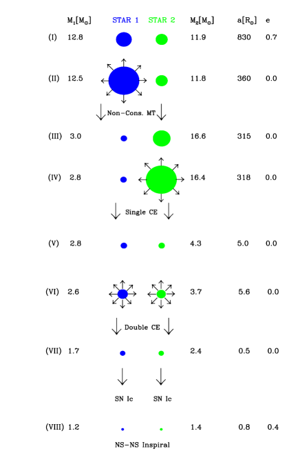
Figure 2: Stages of the new non–recycled NS–NS formation path: (I) Zero Age Main Sequence, (II) star 1 fills its Roche lobe and non–conservative mass transfer begins, (III) at the end of stage II the helium core of Star 1 is exposed, (IV) star 2 fills its Roche lobe on the giant branch leading to dynamically unstable mass transfer and CE evolution, (V) at the end of stage IV the helium core of Star 2 is exposed, (VI) both helium stars fill their Roche lobes on the giant branch, leading to a double CE phase, (VII) at the end of stage VI, the binary consists of two bare CO cores in a tight orbit (VIII) after two subsequent supernovae and 20 Myr since ZAMS a close NS–NS binary forms with a merger time of about 5 Myr. (From Belczynski & Kalogera 2000.)

In Figure 1 we describe in detail the formation of a typical NS–NS binary through this new channel. The evolution begins with two phases of Roche–lobe overflow. The first, from the primary to the secondary, involves non–conservative but dynamically stable mass transfer (stage II) and ends when the hydrogen envelope is consumed. The second, from the initial secondary to the helium core of the initial primary, involves dynamically unstable mass transfer, i.e., CE evolution (stage IV). The post–CE binary consists of two bare helium stars of relatively low masses. As they evolve through core and shell helium burning, the two stars acquire “giant–like” structures, with developed CO cores and convective envelopes (e.g., Habets 1987). Their radial expansion eventually brings them into contact and the system evolves through a double CE phase (stage VI; similar to Brown (1995) for hydrogen–rich stars). During this double CE phase, the combined helium envelopes are ejected at the expense of orbital energy. The tight, post–CE system consists of two CO cores, which eventually end their lives as Type Ic supernovae. The survival probability after the two supernovae is quite high, given the tight orbit before the explosions. The end product in this example is a close NS–NS with a merger time of $\simeq 5$ Myr (typical merger times are found in the range $10^{4}-10^{8}$ yr).

The unique qualitative characteristic of this NS–NS formation path is that both NS have avoided recycling. The NS progenitors have lost both their hydrogen and helium envelopes prior to the two supernovae, so no accretion from winds or Roche–lobe overflow is possible after NS formation. Consequently, these systems are detectable as radio pulsars only for a time ($\sim 10^{6}$ yr) much shorter than recycled NS–NS pulsar lifetimes ($\sim 10^{8}-10^{10}$ yr in the observed sample). Such short lifetimes are of course consistent with the number of NS–NS binaries detected so far and the absence of any non–recycled pulsars among them.

Given the uncertain absolute normalization of population synthesis models, we focus primarily on the formation rate of non–recycled NS–NS binaries relative to that of recycled pulsars, formed through other, qualitatively different evolutionary paths. Based on this comparison, for each of our models, we derive a correction factor for empirical estimates of the Galactic NS–NS coalescence rate. Since these estimates are derived based on the observed sample, they can account only for NS–NS systems with recycled pulsars, and they must be increased to include any non–recycled systems formed. For the majority of the examined models, we find this correction factor to lie in the range $1.5-3$ although for some models it can be as high as 10 or even higher (for more details see Belczynski & Kalogera 2000).

As already mentioned, the realization of the newly identified path through a double helium CE phase depends on the final stages of a helium star evolution. It has long been known that low mass helium stars, after core helium exhaustion, expand significantly and develop a “giant-like” structure with a clearly defined core and a convective envelope (Habets 1987; Avila-Reese 1993; Woosley, Langer, & Weaver 1995; Hurley et al. 2000). We further examined in detail models of evolved helium stars (Woosley 1997, private communication) and found that helium stars below 4.0 M_⊙ have deep convective envelopes and that slightly more massive helium stars ($\sim$ 4–4.5 M_⊙) still form convective envelopes although shallower. Evolved stars with convective envelopes, overfilling Roche lobes in binary systems, transfer mass on a dynamical time scale, and as a consequence CE evolution ensues. The development of CE phases was proposed first in the context of cataclysmic variable formation (Paczynski 1976) and is now supported by detailed hydrodynamic calculations in a variety of binary configurations (e.g. Rasio & Livio 1996; Taam & Sandquist 2000 and references therein). At present no hydro calculations exist for the case of two evolved stars. Based on our basic understanding of CE development, it seems reasonable to expect that, if two stars with convective envelopes are involved in a mass transfer episode, a double core spiral-in can occur leading to double CE ejection (Brown 1995). Based on these earlier calculations, we adopt a maximum helium–star mass for CE evolution (double or single) of 4.5 M_⊙. The formation rates of both types of NS–NS binaries are somewhat sensitive to this value, because they depend on whether helium stars evolve through CE phases (single and double, for recycled and non-recycled systems, respectively). Reducing the maximum mass to 4 M_⊙ actually increases the rate correction factor, although by less than 20%, as it reduces the recycled NS–NS rate by a factor larger than the non–recycled rate.

We note that the identification of the formation path for non–recycled NS–NS binaries stems entirely from accounting for the evolution of helium stars and for the possibility of double CE phases, both of which have typically been ignored in previous calculations (with the exception of Fryer et al. 1999, although formation paths for non–recycled NS–NS were not discussed).

4.2 DISCUSSION

We have identified a new possible evolutionary path leading to the formation of close NS–NS binaries, with the unique characteristic that both NS have avoided recycling by accretion. The realization of this path is related to the evolution of helium–rich stars, and particularly to the radial expansion and development of convective envelopes (on the giant branch) of low–mass ($<4.5$ M_⊙) helium stars. We find that a significant fraction of coalescing NS–NS form through this new channel, for a very wide range of model parameters. In some cases, the non–recycled NS–NS systems strongly dominate the total close NS–NS population.

Since both NS are non–recycled, their pulsar lifetimes are too short (by $\sim 10^{3}$), and hence their detection probability is negligible relative to recycled NS–NS. However, intermediate progenitors of these systems may provide evidence in support of the evolutionary sequence. Examples are close binaries with two low–mass helium stars or a helium star with an O,B companion. Although there are selection effects against their detection too (e.g., short lifetimes, high–mass helium stars are brighter, broad spectral lines due to winds, high luminosity contrast between binary members, etc.), it has been estimated that so far only about 1% of binary helium stars have been detected (Vrancken et al. 1991). Therefore, it is reasonable to expect that the observed sample will increase in future years as observational techniques improve. It is worth noting that theoretical calculations indicate that explosions of low–mass helium stars formed in binaries reproduce the light curves of type Ib supernovae (Shigeyama et al. 1990).

The results of our population modeling show that, if one accounts for the formation of non–recycled NS–NS binaries, the total number of coalescing NS-NS systems could be higher by factors of at least 50%, and up to 10 or even higher. Such an increase has important implications for prospects of gravitational wave detection by ground–based interferometers. Using the results of Kalogera et al. (2000) on the empirical NS–NS coalescence rate, we find that their most optimistic prediction for the LIGO I detection rate could be raised to at least 1 event per 2–3 years, and their most pessimistic LIGO II detection rate could be raised to 3–4 events per year or even higher.

Our results also have important implications for gamma–ray bursts (GRBs), if they are associated with NS–NS coalescence. We find that the typical merger times of the non–recycled NS–NS are considerably shorter than those of recycled binaries, whereas their center–of–mass velocities are higher. The balance of these two competing effects could alter the current consensus for the location of GRB progenitors relative to their host galaxies (e.g., Belczynski, Bulik, & Rudak 2000; Bloom, Kulkarni, & Djorgovski 2000; Fryer et al. 1999).

Acknowledgments

Support is acknowledged by the Smithsonian Institution through a CfA Predoctoral Fellowship to KB and a Clay Fellowship to VK, and by a Polish Nat. Res. Comm. (KBN) grant 2P03D02219 to KB.

References

References

- [1] Avila-Rees, V. A. 1993, Rev. Mex. Astron. Astrofis., 25, 79
- [2] Belczynski, K., Bulik, T., & Rudak, B. 2000, A&A, submitted [astro-ph/0011177]
- [3] Belczynski, K., Kalogera, V. 2000, ApJ Letters, submitted [astro-ph/0012172]
- [4] Belczynski, K., Kalogera, V. & Bulik T., 2001 in preparation
- [5] Blitz, L. 1997, in “CO: Twenty–Five Years of Millimeter-Wave Spectroscopy”, eds. W.B. Latter, et al. (Kluwer Academic Publishers), 11
- [6] Bloom, J.S., Kulkarni, S.R., & Djorgovski, S.G. 2000, ApJ, submitted [astro-ph/0010176]
- [7] Brown, G.E. 1995, ApJ, 440, 270
- [8] Cappellaro, E., Evans, R., & Turatto, M. 1999, ApJ, 351, 459
- [9] Cordes, J., & Chernoff, D.F. 1997, ApJ, 482, 971
- [10] de Donder, E., & Vanbeveren, D. 1998, A&A, 333, 557
- [11] de Kool, M. 1992, A&A, 261, 188
- [12] Dewey, R. J., & Cordes, J. M. 1987, ApJ, 321, 780
- [13] Fryer, C.L., & Kalogera, V. 2001, ApJ, in press [astro-ph/9911312]
- [14] Fryer, C. L., Woosley, S. E., & Hartmann, D. H. 1999, ApJ, 526, 152
- [15] Gilmore, G. 2001, to appear in “Galaxy Disks and Disk Galaxies”, eds. J.G. Funes & E.M. Corsini (San Francisco: ASP)
- [16] Habets, G. M. H. J. 1987, A&A Supplement Series, 69, 183
- [17] Han, Z., Podsiadlowski, P., & Eggleton, P.P. 1995, MNRAS, 272, 800
- [18] Hurley, J.R., Pols, O.R., & Tout, C.A. 2000, MNRAS, 315, 543
- [19] Kalogera, V. 1996, ApJ, 471, 352
- [20] Kalogera, V. 1998, ApJ, 493, 368
- [21] Kalogera, V. 2001, to appear in Workshop on Astrophysical Sources for Ground-Based Gravitational Wave Detectors, ed. J. Centrella
- [22] Kalogera, V., & Baym, G.A. 1996, ApJ, 470, L61
- [23] Kalogera, V., & Lorimer, D.R. 2000, ApJ, 530, 890
- [24] Kalogera, V., Narayan, R., Spergel, D.N., & Taylor, J.H. 2000, ApJ, submitted [astro-ph/0012038]
- [25] Kalogera, V., & Webbink, R.F. 1998, ApJ, 493, 351
- [26] Kolb, U. 1993, A&A, 271, 149
- [27] Lacey, C.G., & Fall, S.M. 1985, ApJ, 290, 154
- [28] Lipunov, V. M., & Postnov, K. A. 1988, Astrophysics & Space Science, 145, 1
- [29] Paczynski, B. 1976, in “The Structure and Evolution of Close Binary Systems”, eds. P. Eggleton, S. Mitton, & J. Whelan, Dordrecht, Reidel, p. 75
- [30] Podsiadlowski, P., Joss, P.C., & Hsu, J.J.L. 1992, ApJ, 391, 246
- [31] Politano, M. J. 1996, ApJ, 465, 338
- [32] Portegies–Zwart, S. F., & Verbunt, F. 1996, A&A, 309, 179
- [33] Portegies–Zwart, S. F., & Yungel’son, L. R. 1998, A&A, 332, 173
- [34] Rasio, F. A., & Livio, M. 1996, ApJ, 471, 366
- [35] Schaller, G., Schaerer, D., Meynet, G., & Maeder, A. 1992, A&A Supplement Series, 269, 331
- [36] Shigeyama, T., Nomoto, K., Tsujimoto, T., & Hashimoto, M. 1990, ApJ, 361, L23
- [37] Tamm, R. E., & Sandquist, E. L. 2000, ARA&A, 38, 113
- [38] Vrancken, J., DeGreve, J.P., Yungel’son, L., & Tutukov, A. 1991, A&A, 249, 411
- [39] Webbink, R.F. 1984, ApJ, 277, 355
- [40] Woosley, S.E. 1986, in “Nucleosynthesis and Chemical Evolution”, 16th Saas-Fee Course, eds. B. Hauck et al., Geneva Obs., p. 1
- [41] Woosley, S. E., Langer, N., & Weaver, T. A. 1995, ApJ, 448, 315